Approximate solutions for mixed nonlinear Volterra–Fredholm type integral equations via modified block-pulse functions

Abstract

In this article a robust approach for solving mixed nonlinear Volterra–Fredholm type integral equations of the first kind is investigated. By using the modified two-dimensional block-pulse functions (M2D-BFs) and their operational matrix of integration, first kind mixed nonlinear Volterra–Fredholm type integral equations can by reduced to a nonlinear system of equations. The coefficients matrix of this system is a block matrix with lower triangular blocks. Some theorems are included to show the convergence and advantage of this method. Numerical results show that the approximate solutions have a good degree of accuracy.

Keywords:

• Mixed nonlinear Volterra–Fredholm type integral equations
• Block-pulse functions
• Operational matrix

1 Introduction

In this paper we applied the direct method for solving mixed nonlinear Volterra–Fredholm type integral equations of the first kind of the form:(1) where u(s,t) is an unknown function, f(x,y) and G(x,y,s,t,u(s,t)) are analytical function on [0,1) × Ω and [0,1) × Ω⁴, respectively, where Ω is a close subset on . Existence and uniqueness results for Eq. (1)(1) may be found in (Diekmann, 1978; Pachpatte, 1978; Thieme, 1977).

Equation of type (1)(1) often arise from the mathematical modeling of the spreading, in space and time, of some contagious disease in a population living in a habitat Ω (Diekmann, 1978; Thieme, 1977), in the theory of nonlinear parabolic boundary value problems (Pachpatte, 1978), and in many physical and biological models.

The literature on numerical methods for solving Eq. (1)(1) mainly consists of projection methods, collocation methods, the trapezoidal Nyström method, Adomain decomposition method, He’s homotopy perturbation method and the two-dimensional block-pulse functions (Adomian, 1990, 1994; Adomian and Rach, 1992; Biazar et al., 2011; Brunner, 1990; Cardone et al., 2006; Cherruault et al., 1992; Guoqiang, 1995; Hacia, 1996; Kauthen, 1989; Maleknejad and Fadaei Yami, 2006; Maleknejad and Hadizadeh, 1999; Maleknejad and Mahdiani, 2011; Wazwaz, 2006; Yee, 1993).

Assume now that:(2) where p is a positive integer. In the present paper, we apply a modification of block-pulse functions (Maleknejad and Rahimi, 2011), to solve the mixed nonlinear Volterra–Fredholm type integral Eq. (1)(1) with Eq. (2)(2) .

2 M2D-BFs and their properties

Definition 1

An (m + 1)²-set of M2D-BFs consists of (m + 1)² functions which are defined over district D = [0,1) × [0,1) as follows:(3) where , and(4) where m is an arbitrary positive integer, and .

Since, each M2D-BF takes only one value in its subregion, the M2D-BFs can be expressed by the two modified one-dimensional block-pulse functions (M1D-BFs):(5) where and are the M1D-BFs related to variables x and y, respectively. The M2D-BFs are disjointed with each other:(6) and are orthogonal with each other:(7) where (x,y) ∈ D, i₁,i₂,j₁,j₂ = 0(1)m and and are length of intervals and , respectively.

2.1 Vector forms

Consider the first (m + 1)² terms of M2D-BFs and write them concisely as (m + 1)²-vector:(8) Whence Eqs. (6)(6) and (8)(8) implies that:(9) Now suppose that X be a (m + 1)²-vector. Hence by using Eq. (9)(9) we obtain:(10) where is a (m + 1)² × (m + 1)² diagonal matrix.

2.2 M2D-BFs expansions

A function f(x,y) defined over district L²(D) may be expanded by the M2D-BFs as:(11) where F_m,ɛ is an (m + 1)² × 1 vector given by(12) and Φ_m,ɛ(x,y) is defined in Eq. (8)(8) , and , are obtained as:(13) Similarly a function of four variables, k(x,y,s,t), on district L²(D × D) may be approximated with respect to M2D-BFs such as:(14) where Φ_m,ɛ(x,y) and Φ_m,ɛ(s,t) are M2D-BFs vector of dimension (m + 1)², and K_m,ɛ is the (m + 1)² × (m + 1)² M2D-BFs coefficients matrix.

3 Convergence analysis

In this section, we show that the given method in the previous sections, is convergent and its order of convergence is . For our purposes we will need the following theorems.

Theorem 1

LetandThen the following equation(15) achieves its minimum value and also we have(16)

Proof

It is an immediate consequence of theorem which was proved by Jiang and Schaufelberger (1992).□

Theorem 2

Assume f(x,y) is continuous and is differentiable over district [−h,1 + h] × [−h,1 + h], and for i = 0(1)(k − 1), are correspondingly M2D-BFs(ɛ₀) = 2D-BFs, M2D-BFs(ɛ₁), …, M2D-BFs(ɛ_k−1) expansions of f(x, y) based on (m + 1)² M2D-BFs over district D andthen for sufficient large m we have:

Proof

We consider and in the district which are approximately equal to constants n₁ and n₂, respectively, where m is so large. Also, we use page z = n₁x + n₂y + b instead of f(x,y) in the district . Now in the district we have:(17) but and Eq. (17)(17) can be reformulated as:(18) In other words:(19) so, we have:(20) where .

By using Eqs. (19)(19) and (20)(20) the proof is completed.□

Theorem 3

Let the representation error between f(x,y) and its two-dimensional block-pulse functions, (M2D-BFs, over the district D, as follows:Then and

Proof

See (Maleknejad et al., 2010).□

Theorems 2 and 3 conclude that error estimation for M2D-BFs is .

If we assume E₁ and E₂ are errors between f(x,y) and its 2D-BFs and M2D-BFs expansions, respectively, from Theorem 2 we have , and from (Maleknejad et al., 2010) we have , where M is bounded of ∥Df(x,y)∥ and m shows number of 2D-BFs.

So, we have(21) where k is times of modifications of the M2D-BFs series.

Assume now that f(x,y) is approximated bywhereas, are the approximation of andthen for we have(22) We have(23) Consequently by using Eqs. (21)–(23), the following error bound is obtained:(24) Moreover Eq. (24)(24) implies that:(25)

4 Method of solution

In this section, we solve mixed nonlinear Volterra–Fredholm type integral equations of the first kind of the form Eq. (1)(1) with Eq. (2)(2) by using M2D-BFs.

We now approximate functions u(x,y),f(x,y),[u(x,y)]^p and k(x,y,s,t) with respect to M2D-BFs by manipulation as Section 2:(26) where Φ_m,ɛ(x,y) is defined in Eq. (8)(8) , the vectors U_m,ɛ, F_m,ɛ, U_m,ɛ,p, and matrix K_m,ɛ are M2D-BFs coefficients of u(x,y),f(x,y), [u(x,y)]^p and k(x,y,s,t) respectively.

Lemma 1

Let (m + 1)²-vectors U_m,ɛ and U_m,ɛ,p be M2D-BFs coefficients of u(x,y) and [u(x,y)]^p, respectively. If(27) then we have:(28) where p ⩾ 1, is a positive integer.

Proof

(By induction) When p = 1, Eq. (28)(28) follows at once from [u(x,y)]^p = u(x,y). Suppose that Eq. (28)(28) holds for p, we shall deduce it for (p + 1). Since [u(x,y)]^p+1 = u(x,y)[u(x,y)]^p, from Eqs. (26)(26) and (10)(10) it follows that(29) Now by using Eq. (28)(28) we obtain(30) therefore Eq. (28)(28) holds for (p + 1), and the lemma is established.□

To approximate the integral part in Eq. (1)(1) with Eq. (2)(2) , from Eq. (26)(26) we get(31) Now by using Eqs. (5)(5) and (9)(9) , denoting R_j for the (j + 1)th row of the conventional integration operational matrix P_m,ɛ ((P_m,ɛ)_(m+1)×(m+1) is operational matrix of 1D-BFs defined over [0,1), see Maleknejad and Mahdiani, 2011) and considering follows:(32) Also by using Eq. (5), Eq. (8) can be reformulated as:(33) So, we have(34) Also, we have:(35) By using Eqs. (32), (34)(32) and (35)(34) , Eq. (31)(31) can be reformulated as:(36) where(37) whereand 0 is a zero matrix. Also(38) where(39) (40) So, we have :(41) Substituting Eqs. (26)(26) and (41)(41) into Eq. (1)(1) with Eq. (2)(2) gives:(42) After solving the above nonlinear system by using Newton–Raphson method, we can find U_m,ɛ and then(43) Then(44) where is the estimation of the solution of mixed nonlinear Volterra–Fredholm type integral equation of the first kind.

5 Numerical examples

In this section to demonstrate the effectiveness of our approach several examples are presented. All results are computed by using a program written in the Matlab. The numerical experiments are carried our for the selected grid point which are proposed as (2^−l; l = 1,2,3,4) and m terms and k times of modifications of the M2D-BFs series. The following problems have been tested.

Example 1

Consider the following mixed linear Volterra–Fredholm type integral equation (Maleknejad and Mahdiani, 2011):(45) where(46) The exact solution is u(x,y) = e^−xcos(y). Table 1 and Fig. 1 illustrate the numerical results for this example.

The error results for proposed method besides the error for method of Maleknejad and Mahdiani (2011) are tabulated in Table 2.

Example 2

Consider the following mixed nonlinear Volterra–Fredholm type integral equation (Maleknejad and Mahdiani, 2011):(47) where(48) The exact solution is u(x,y) = e^−x−y. Table 3 and Fig. 2 illustrate the numerical results for this example.

The error results for proposed method besides the error for method of Maleknejad and Mahdiani (2011) are tabulated in Table 4.

Figure 1 Absolute value of error, Example 1 with m = 8 and k = 1,2,3.

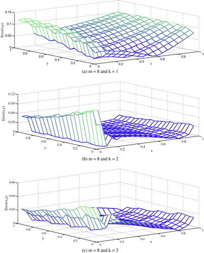
Figure 2 Absolute value of error, Example 2 with m = 8 and k = 1,2,3.

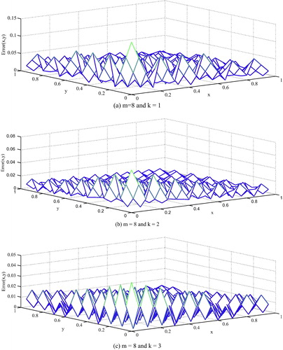
Table 1 Numerical results of Example 1 with M2D-BFs.

Nodes	Error for
	k = 1	k = 2	k = 3
l = 1	0.03748936	0.02837304	0.02522153
l = 2	0.05090571	0.03943282	0.03190341
l = 3	0.02574872	0.01813532	0.01391462
l = 4	0.04112879	0.02553757	0.02222506

Table 2 Error results for Example 1.

Nodes	Present method	Method of Maleknejad and Mahdiani (2011)
	m = 8 and k = 2	m = 16
l = 1	0.02837304	0.0288649
l = 2	0.03943282	0.0398778
l = 3	0.01813532	0.0310669
l = 4	0.02553757	0.0277814

Table 3 Numerical results of Example 2 with M2D-BFs.

Nodes	Error for m = 8
	k = 1	k = 2	k = 3
l = 1	0.04289052	0.03148406	0.02743874
l = 2	0.06470576	0.04585369	0.04071913
l = 3	0.03803418	0.02437943	0.02249845
l = 4	0.03592263	0.02836157	0.02045372

Table 4 Error results for Example 2.

Nodes	Present method	Method of Maleknejad and Mahdiani (2011)
	m = 8 and k = 2	m = 16
l = 1	0.03148406	0.04289006
l = 2	0.04585369	0.04589757
l = 3	0.02437943	0.04034072
l = 4	0.02836157	0.04312157

6 Conclusion

In this paper a computational method for approximate solution of mixed nonlinear Volterra–Fredholm type integral equations of the first kind, based on the expansion of the solution as series of M2D-BFs was presented. This method converts a mixed nonlinear Volterra–Fredholm type integral equation whose answer is the coefficients of M2D-BFs expansion of the solution of mixed nonlinear Volterra–Fredholm type integral equation. Also, we have shown that our approach is convergent and its order of convergence is . This method can be easily extended and applied to mixed nonlinear Volterra–Fredholm type integral equations of the second kind and nonlinear system of the mixed Volterra–Fredholm type integral equations.