Some new exact traveling wave solutions to the simplified MCH equation and the (1 + 1)-dimensional combined KdV–mKdV equations

Peer review under responsibility of University of Bahrain.

Abstract

The generalized (G′/G)-expansion method is thriving in finding exact traveling wave solutions of nonlinear evolution equations (NLEEs) in mathematical physics. In this paper, we bring to bear the generalized (G′/G)-expansion method to look for the exact solutions via the simplified MCH equation and the (1 + 1)-dimensional combined KdV–mKdV equations involving parameters. When the parameters take special values, solitary wave solutions are originated from the traveling wave solutions. It is established that the generalized (G′/G)-expansion method offers a further influential mathematical tool for constructing the exact solutions of NLEEs in mathematical physics.

Keywords:

• The generalized (G′/G)-expansion method
• The simplified MCH equation and the (1 + 1)-dimensional combined KdV–mKdV equations
• Traveling wave solutions
• Solitary wave solutions

1 Introduction

The importance of nonlinear evolution equations (NLEEs) is now well established, since these equations arise in various areas of science and engineering, especially in fluid mechanics, biology, plasma physics, solid-state physics, optical fibers, biophysics and so on. As a key problem, finding their analytical solutions is of great importance and is actually executed through various efficient and powerful methods such as the Miura transformation (Bock and Kruskal, 1979), the Jacobi elliptic function expansion method (Chen and Wang, 2005; Honga and Lub, 2012), the Adomian decomposition method (Adomain, 1994; Wazwaz, 2002), the method of bifurcation of planar dynamical systems (Li and Liu, 2000; Liu and Qian, 2001), the ansatz method (Hu, 2001), the Cole–Hopf transformation (Salas and Gomez, 2010), the (G′/G)-expansion method (Zayed and Gepreel, 2009a,b; Zayed, 2009; Wang et al., 2008; Taha and Noorani, 2013a,b; Akbar et al., 2012a,b,c; Song and Ge, 2010), the (G′/G, 1/G)-expansion method (Zayed et al., 2012; Zayed and Ibrahim, 2013; Zayed and Abdelaziz, 2012; Yang, 2013), the improved (G′/G)-expansion method (Zhang et al., 2010), the modified simple equation method (Jawad et al., 2010; Khan et al., 2013; Khan and Akbar, 2013), the novel (G′/G)-expansion method (Alam et al., 2014; Alam and Akbar, 2014), the new generalized (G′/G)-expansion method (Naher and Abdullah, 2013) and so on.

The objective of this article is to search for new study relating to the generalized (G′/G)-expansion method for solving the simplified MCH equation and the (1 + 1)-dimensional combined KdV–mKdV equations to demonstrate the suitability and straightforwardness of the method.

The article is organized as follows: in Section 2, we describe this method for finding exact traveling wave solutions of nonlinear evolution equations. In Section 3, we will apply this method to obtain the traveling wave solutions of the simplified MCH equation and the (1 + 1)-dimensional combined KdV–mKdV equations. In Section 4, physical explanations are offered. In Section 5 comparison and in Section 6 conclusions are conferred.

2 Material and method

In this section we describe the generalized (G′/G) expansion method for finding traveling wave solutions of nonlinear evolution equations. Let us consider a general nonlinear PDE in the form(1) where u = u(x, t) is an unknown function, P is a polynomial in u(x, t) and its derivatives in which highest order derivatives and nonlinear terms are involved and the subscripts stand for the partial derivatives.

Step 1: We combine the real variables x and t by a complex variable Φ(2) where V is the speed of the traveling wave. The traveling wave transformation (2) converts Eq. (1)(1) into an ordinary differential equation (ODE) for u = u(Φ):(3) where Q is a polynomial of u and its derivatives and the superscripts indicate the ordinary derivatives with respect to Φ.

Step 2: According to possibility Eq. (3)(3) can be integrated term by term one or more times, yields constant(s) of integration. The integral constant may be zero, for simplicity.

Step 3: Suppose the traveling wave solution of Eq. (3)(3) can be expressed as follows:(4) where either a_N or b_N may be zero, but both a_N or b_N could be zero at a time, a_i (i = 0, 1, 2, , N) and b_i (i = 1, 2, , N) and d are arbitrary constants to be determined later and H(Φ) is(5) where G = G(Φ) satisfies the following auxiliary ordinary differential equation:(6) Eq. (6)(6) has individual five solutions (see Lanlan and Huaitang, 2013)where the prime stands for derivative with respect to Φ; A, B,C and E are real parameters.

Step 4: To determine the positive integer N, taking the homogeneous balance between the highest order nonlinear terms and the derivatives of the highest order appearing in Eq. (3)(3) .

Step 5: Substitute Eq. (4)(4) and Eq. (6)(6) including Eq. (5)(5) into Eq. (3)(3) with the value of N obtained in Step 4, we obtain polynomials in (d + H)^N (N = 0,1,2, ) and (d + H)^−N (N = 0,1,2, ). Then, we collect each coefficient of the resulted polynomials to zero, yields a set of algebraic equations for a_i (i = 0,1,2, , N) and b_i (i = 1,2, , N), d and V.

Step 6: Suppose that the value of the constants a_i (i = 0,1,2, , N), b_i (i = 1,2, , N), d and V can be found by solving the algebraic equations obtained in Step 5. Since the general solution of Eq. (6)(6) is well known to us, inserting the values of a_i (i = 0,1,2, , N), b_i (i = 1,2, , N), d and V into Eq. (4)(4) , we obtain more general type and new exact traveling wave solutions of the nonlinear partial differential equation (1)(1) .

Using the general solution of Eq. (6)(6) , we have the following solutions of Eq. (5)(5) :

Family 1: When B ≠ 0, ψ = A − C and Ω = B² + 4E(A − C) > 0,(7)

Family 2: When B ≠ 0, ψ = A − C and Ω = B² + 4E(A − C) < 0,(8)

Family 3: When B ≠ 0, ψ = A − C and Ω = B² + 4E(A − C) = 0,(9)

Family 4: When B = 0, ψ = A − C and Δ = ψE > 0,(10)

Family 5: When B = 0, ψ = A − C and Δ = ψE < 0,(11)

3 Applications

In this section, we will apply the generalized (G′/G) expansion method to find the exact solutions and the solitary wave solutions of the following two nonlinear evolution equations.

3.1 The simplified MCH equation

Now we will bring to bear the generalized (G′/G) expansion method to find exact solutions and then the solitary wave solutions of the simplified MCH equation in the form,(12)

Details of CH and MCH equations can be found in references (Liu et al., 2010: Wazwaz, 2005; Camassa and Holm, 1993; Tian and Song, 2004; Boyd, 1997).

Now, we use the traveling wave transformation Eq. (2)(2) into Eq. (12)(12) , which yields(13) where the superscripts stand for the derivatives with respect to Φ.

Integrating Eq. (13)(13) once with respect to Φ yields:(14) where P is an integral constant that could be determined later.

Taking the homogeneous balance between u³ and in Eq. (14)(14) , we obtain N = 1. Therefore, the solution of Eq. (14)(14) is of the form(15) where a₀, a₁, b₁ and d are constants to be determined.

Substituting Eq. (15)(15) together with Eqs. (5)(5) and (6)(6) into Eq. (14)(14) , the left-hand side is converted into polynomials in (d + H)^N (N = 0,1,2, ) and (d + H)^−N (N = 0,1,2, ). We collect each coefficient of these resulted polynomials to zero, yields a set of simultaneous algebraic equations (for simplicity which are not presented here) for a₀, a₁, b₁, d and V. Solving these algebraic equations with the help of symbolic computation software, we obtain following:(16) where A, B, C and E are free parameters.

Substituting Eq. (16)(16) into Eq. (15)(15) , along with Eq. (7)(7) and simplifying yields following traveling wave solutions (if C₁ = 0 but C₂ ≠ 0 and C₂ = 0 but C₁ ≠ 0), respectively:where .

Substituting Eq. (16)(16) into Eq. (15)(15) , along with Eq. (8)(8) and simplifying, the obtained exact solutions become (if C₁ = 0 but C₂ ≠ 0; C₂ = 0 but C₁ ≠ 0), respectively:

Substituting Eq. (16)(16) into Eq. (15)(15) together with Eq. (9)(9) and simplifying, we obtain

Substituting Eq. (16)(16) into Eq. (15)(15) , along with Eq. (10)(10) and simplifying, we obtain following traveling wave solutions (if C₁ = 0 but C₂ ≠ 0; C₂ = 0 but C₁ ≠ 0), respectively:

Substituting Eq. (16)(16) into Eq. (15)(15) , together with Eq. (11)(11) and simplifying, our obtained exact solutions become (if C₁ = 0 but C₂ ≠ 0; C₂ = 0 but C₁ ≠ 0), respectively:

3.2 The (1 + 1)-dimensional combined KdV–mKdV equation

In this section, we will apply the generalized (G′/G) expansion method to find exact solutions and then the solitary wave solutions of the (1 + 1)-dimensional combined KdV–mKdV equation (Zayed, 2011) in the form,(17) where α and β are nonzero constants. This equation may describe the wave propagation of the bound particle, sound wave and thermal pulse. This equation is the most popular soliton equation and often exists in practical problems such as fluid physics and quantum field theory.

The wave transformation equation u(Φ) = u(x,t), Φ = x − Vt. Reduces Eq. (17)(17) into the following ODE:(18) where the superscripts stand for the derivatives with respect to Φ.Integrating Eq. (18)(18) once with respect to Φ yields:(19) where P is an integral constant that could be determined later.

Taking the homogeneous balance between u³ and in Eq. (19)(19) , we obtain N = 1. Therefore, the solution of Eq. (19)(19) is of the form(20) where a₀, a₁, b₁ and d are constants to be determined.

Substituting Eq. (20)(20) together with Eqs. (5)(5) and (6)(6) into Eq. (19)(19) , the left-hand side is converted into polynomials in (d + H)^N (N = 0,1,2, ) and (d + H)^−N (N = 0,1,2,). We collect each coefficient of these resulted polynomials to zero, yields a set of simultaneous algebraic equations (for simplicity which are not presented here) for a₀, a₁, b₁, d and V. Solving these algebraic equations with the help of symbolic computation software, we obtain following:(21) where ψ = A − C, , m₂ = −(Aαm₁ − 12dψ − 6B) A, B, C and E are free parameters.

Substituting Eq. (21)(21) into Eq. (20)(20) , along with Eq. (7)(7) and simplifying yields following traveling wave solutions (if C₁ = 0 but C₂ ≠ 0 and C₂ = 0 but C₁ ≠ 0), respectively:where .

Substituting Eq. (21)(21) into Eq. (20)(20) , along with Eq. (8)(8) and simplifying, the obtained exact solutions become (if C₁ = 0 but C₂ ≠ 0;C₂ = 0 but C₁ ≠ 0), respectively:

Substituting Eq. (21)(21) into Eq. (20)(20) together with Eq. (9)(9) and simplifying, we obtain

Substituting Eq. (21)(21) into Eq. (20)(20) , along with Eq. (10)(10) and simplifying, we obtain following traveling wave solutions (if C₁ = 0 but C₂ ≠ 0;C₂ = 0 but C₁ ≠ 0), respectively:

Substituting Eq. (21)(21) into Eq. (20)(20) , together with Eq. (11)(11) and simplifying, our obtained exact solutions become (if C₁ = 0 but C₂ ≠ 0; C₂ = 0 but C₁ ≠ 0), respectively:

4 Physical explanation

In this section we will put forth the physical significances and graphical representations of the obtained results of the simplified MCH equation and the (1 + 1)-dimensional combined KdV–mKdV equation.

4.1 Results and discussion

i.

Solutions u1(Φ), u2(Φ), u6(Φ), u7(Φ), u10(Φ), u11(Φ), u15(Φ) and u16(Φ) are hyperbolic function solutions. Solutions u1(Φ), u6(Φ), u10(Φ) and u15(Φ) are the single soliton solution. Fig. 1 shows the shape of the exact single soliton solution (only shows the shape of solution of u10(Φ) with A = 4, B = 1, C = 1, E = 1, α = 1, β = 1, d = 1 with −10 ⩽ x, t ⩽ 10). The shape of figure of solutions u1(Φ), u6(Φ) and u15(Φ) are similar to the figure of solution u10(Φ). Solutions u2(Φ) and u7(Φ) are the singular soliton solution. Fig. 2 shows the shape of the exact singular soliton solution (only shows the shape of solution of u7(Φ) with A = 2, B = 0, C = 1, E = 1, k = 1, β = 1, d = 1 with −10 ⩽ x, t ⩽ 10). The shape of figure of solutions u2(Φ) are similar to the figure of solution u7(Φ). Solutions u11(Φ) and u16(Φ) are the Kink solutions. Fig. 3 shows the shape of the exact Kink solution (only shows the shape of solution of u11(Φ) with A = 2, B = 0, C = 1, E = 1, α = 1, β = 1, d = 1 with −10 ⩽ x, t ⩽ 10).

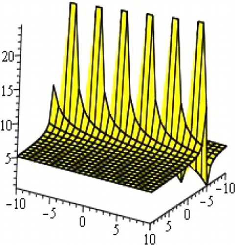
ii.

Solutions u3(Φ), u4(Φ), u8(Φ), u9(Φ), u12(Φ), u13(Φ), u17(Φ) and u18(Φ) are trigonometric function solutions. Solutions u3(Φ) and u12(Φ) are the single soliton solution. The shape of figure of solutions u3(Φ) and u12(Φ) are similar to the figure of solution u10(Φ). Solutions u4(Φ), u13(Φ), u17(Φ), u9(Φ) and u18(Φ) are the exact periodic traveling wave solutions. Fig. 4 below shows the periodic solution of u9(Φ). Graph of periodic solution of u9(Φ), for A = 1, B = 0, C = 2, E = 2, k = 1, d = 1, β = 1 with −5 ⩽ x, t ⩽ 5. For convenience the figure is omitted. Solution u8(Φ) is the multiple soliton solution. Fig. 5 shows the shape of the exact singular soliton solution (only shows the shape of solution of u8(Φ) with A = 1, B = 0, C = 2, E = 1, k = 1, β = 1, d = 1 with −1 ⩽ x, t ⩽ 1).

iii.

Solutions u5(Φ) and u14(Φ) are complex rational traveling wave solutions. Solution u5(Φ) is the single soliton solution. The shape of figure of solution u5(Φ) is similar to the figure of solution u10(Φ). Fig. 6 shows the shape of the exact singular Kink solution (only shows the shape of solution of u14(Φ) with A = 1, B = 2, C = 2, E = 1, α = 1, d = 1, C1 = 2, C2 = 1, β = 1 with −10 ⩽ x, t ⩽ 10).

Figure 1 Single soliton wave, the shape of solution of u₁₀(Φ) with A = 4, B = 1, C = 1, E = 1, α = 1, β = 1, d = 1 with −10 ⩽ x, t ⩽ 10.

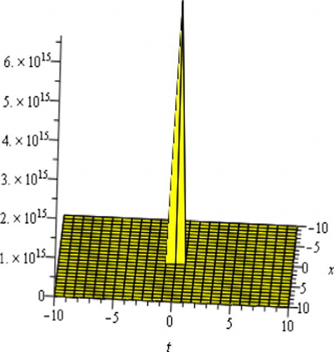
Figure 2 Singular soliton, the shape of solution of u₇(Φ) with A = 2, B = 0, C = 1, E = 1, k = 1, β = 1, d = 1 with −10 ⩽ x, t ⩽ 10.

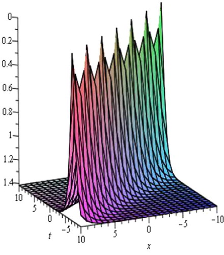
Figure 3 Kink solution, the shape of solution of u₁₁(Φ) with A = 2, B = 0, C = 1, E = 1, α = 1, β = 1, d = 1 with −10 ⩽ x, t ⩽ 10.

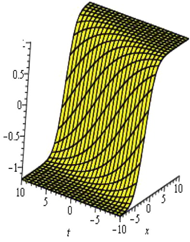
Figure 4 Periodic solutions of u₉(Φ), for A = 1, B = 0, C = 2, E = 2, k = 1, d = 1, β = 1 with −5 ⩽ x, t ⩽ 5.

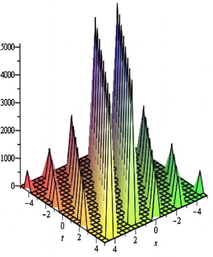
Figure 5 Multiple soliton solution, the shape of solution of u₈(Φ) with A = 1, B = 0, C = 2, E = 1, k = 1, β = 1, d = 1 with −1 ⩽ x, t ⩽ 1.

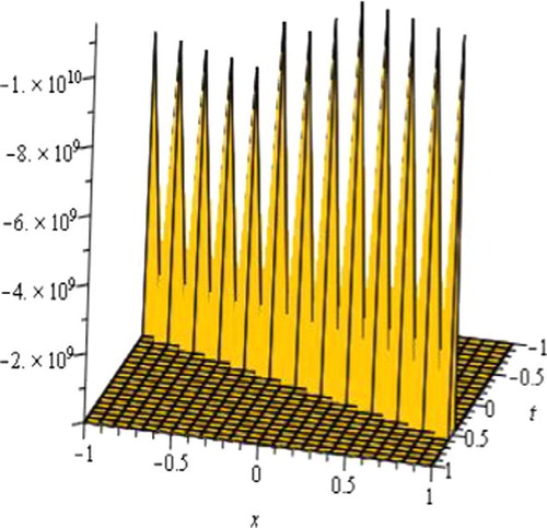
Figure 6 Singular Kink solution, the shape of solution of u₁₄(Φ) with A = 1, B = 2, C = 2, E = 1, α = 1, d = 1, C₁ = 2, C₂ = 1, β = 1 with −10 ⩽ x, t ⩽ 10.

4.2 Graphical representation

The graphical demonstrations of obtained solutions for particular values of the arbitrary constants are shown in Figs. 1–6 with the aid of commercial software Maple.

5 Comparison

5.1 Comparison between Zayed (2011) solutions and our solutions

Zayed (2011) considered solutions of the (1 + 1)-dimensional combined KdV–mKdV equation using the basic (G′/G)-expansion method combined with the Riccati equation. The solutions of the (1 + 1)-dimensional combined KdV–mKdV equation obtained by the generalized (G′/G)-expansion method are different from those of the basic (G′/G)-expansion method combined with the Riccati equation. Moreover, in Zayed (2011) investigated the well-established (1 + 1)-dimensional combined KdV–mKdV equation to obtain exact solutions via the basic (G′/G)-expansion method and achieved only seven solutions (see Appendix). Furthermore, nine solutions of the well-known (1 + 1)-dimensional combined KdV–mKdV equation is constructed by applying the generalized (G′/G)-expansion method. On the other hand, the auxiliary equation used in this paper is different, so obtained solutions is also different. Similarly for any nonlinear evolution equation it can be shown that the generalized (G′/G)-expansion method is much easier than other methods.

5.2 Comparison between Liu et al. (2010) solutions and our solutions

Liu et al. (2010) investigated solutions of the well-established simplified MCH equation via the (G′/G)-expansion method wherein he used the linear ordinary differential equation as auxiliary equation and traveling wave solution was presented in the form where a_m ≠ 0. It is noteworthy to point out that some of our solutions are coincided with already published results, if parameters taken particular values which authenticate our solutions. The comparison of Liu et al. (2010) and the solutions obtained in this article are given in: Table 1

Table 1 Comparison between Liu et al. (2010) solutions and our solutions.

Liu et al. (2010) solutions	Obtained solutions
i. If C1 = 0, solutions Eq. (3.8) becomes: .	i. If d = 0, B = 0, A = 1, u1(ϕ)=u1,2(ξ), β = a, E = -μ, and then the solution is .
ii. If C1 = 0, solutions Eq. (3.8) becomes:	ii. If and then the solution is
iii. If , solutions Eq. (3.8) becomes:	iii. If and C = 0 then the solution is
iv. If C1 = 0, solutions Eq. (3.10) becomes:	iv. If and then the solution is
v. If C1 = 0, solutions Eq. (3.10) becomes:	v. If and then the solution is
vi. If , solutions Eq. (3.10) becomes:	vi. If and C = 0 then the solution is

In addition to this table, we obtain further new exact traveling wave solutions u₂(Φ), u₄(Φ), u₇(Φ) and u₉(Φ), which are not reported in the previous literature (Liu et al., 2010). When the arbitrary constants assume particular values the obtained solutions reduce to some special functions. On the other hand, the auxiliary equation used in this paper is different, so obtained solutions is also different.

6 Conclusion

Some new exact traveling wave solutions of the simplified MCH equation and the (1 + 1)-dimensional combined KdV–mKdV equations are constructed in this article by applying the generalized (G′/G)-expansion method. The obtained solutions are presented in terms of hyperbolic, trigonometric and rational functions. Also, the solutions show that the application of the method is trustworthy, straightforward and gives many solutions. We have noted that the generalized (G′/G)-expansion method changes the given difficult problems into simple problems which can be solved easily. We hope this method can be more effectively used to solve many nonlinear partial differential equations in applied mathematics, engineering and mathematical physics.

Acknowledgments

The authors would like to express their sincere thanks to the anonymous referee(s) for their detail comments and valuable suggestions.

Notes

Peer review under responsibility of University of Bahrain.

Appendix A

Zayed (2011) studied solutions of the (1 + 1)-dimensional combined KdV–mKdV equation using the basic (G′/G)-expansion method combined with the Riccati equation and achieved the following calculations and exact solutions:(6)

Consequently the following algebraic equations(7)

Which can be solved to get(8)

Substituting (3.8) into (3.4) yields(9) Where(10)

According to general solutions of the Riccati equations, (Zayed, 2011) got the following families of exact solutions:

Family 1. If , then(11) Or(12) Where and

Family 2. If then(13) Or(14) Where .

Family 3. If A = 1, B = −1, then(15) Where .

Family 4. If A = B = 1, then(16) Where .

Family 5. If A = 0, B ≠ 0, then(17) where .

The general solutions of the Riccati equations are well known which are listed in the following table:

Table

A	B	The solution G(ξ)
1	−1	tanh ξ, coth ξ
1	1	tan ξ, −cot ξ
0	≠0	, where c1 is an arbitrary constant.