Numerical computation of fractional multi-dimensional diffusion equations by using a modified homotopy perturbation method

Peer review under responsibility of University of Bahrain.

Abstract

The main aim of the present work is to present a numerical algorithm for solving fractional multi-dimensional diffusion equations which describes density dynamics in a material undergoing diffusion by using a modified homotopy perturbation method with the help of the sumudu transform. The modified homotopy perturbation method is not limited to the small parameter, such as in the classical perturbation method. The method gives an analytical solution in the form of a convergent series with easily computable components, requiring no linearization or small perturbation. The numerical results obtained by the proposed method indicate that the approach is easy to implement and computationally very attractive.

Keywords:

• Modified homotopy perturbation method
• Sumudu transform
• Fractional multi-dimensional diffusion equations
• He’s polynomials

1 Introduction

The diffusion equation is a partial differential equation which describes density dynamics in a material undergoing diffusion. It is also used to describe processes exhibiting diffusive-like behaviour, for instance the ‘diffusion’ of alleles in a population in population genetics. The equation can be written as,(1) where U(r, t) is the density of the diffusing material at location r = (x, y, z) and time t. D(U(r, t), r) denotes the collective diffusion coefficient for density U at location r. Several techniques including the numerical method (Siddique, 2010), variational iteration method (Akbarzade and Langari, 2011) and homotopy perturbation method (Akbarzade and Langari, 2011) have been used for solving these type of problems and references therein.

In recent years, fractional differential equations have gained importance and popularity, mainly due to their demonstrated applications in science and engineering. For example, these equations are increasingly used to model problems in research areas as diverse as dynamical systems, mechanical systems, control, chaos, chaos synchronization, continuous-time random walks, anomalous diffusive and subdiffusive systems, unification of diffusion and wave propagation phenomenon and others (Young, 1995; Hilfer, 2000; Podlubny, 1999; Mainardi et al., 2001; Debnath, 2003; Caputo, 1969; Miller and Ross, 1993; Oldham and Spanier, 1974; Kilbas et al., 2006).

The homotopy perturbation method (HPM) was first introduced by Chinese researcher J.H. He in 1998 and was developed by him (He, 1999, 2003, 2006). The HPM was also studied by many authors to handle nonlinear equations arising in science and engineering (Ganji, 2006; Ganji et al., 2010; Jafari et al., 2008; Rashidi et al., 2009; Rashidi and Ganji, 2009; Yildirim, 2009; Kumar and Singh, 2010; Atangana and Secer, 2013). In recent years, many authors have paid attention to study the solutions of linear and nonlinear partial differential equations by using various methods combined with the Laplace transform (Khuri, 2001; Khan and Hussain, 2011; Khan et al., 2012; Gondal and Khan, 2010; Kumar et al., 2012) and sumudu transform (Singh et al., 2011, 2013; Sushila et al., 2013; Atangana and Kilicman, 2013; Atangana and Baleanu, 2013).

In this paper, we implement the modified homotopy perturbation method with the help of the sumudu transform for obtaining analytical and numerical solutions of the fractional multi-dimensional diffusion equations. The present modification is similar to the modified homotopy perturbation method with help of the Laplace transform (Gondal and Khan, 2010; Kumar et al., 2012). The advantage of this technique is its capability of combining two powerful methods for obtaining exact and approximate analytical solutions for nonlinear equations. It is worth mentioning that the proposed method is capable of reducing the volume of the computational work as compared to the classical methods while still maintaining the high accuracy of the numerical result; the size reduction amounts to an improvement of the performance of the approach.

2 Basic definitions of fractional calculus

In this section, we mention the following basic definitions of fractional calculus.

Definition 1

The Riemann–Liouville fractional integral operator of order α > 0, of a function is defined as (Podlubny, 1999):(2)

(3) For the Riemann–Liouville fractional integral we have:(4)

Definition 2

The fractional derivative of f(t) in the Caputo sense is defined as (Caputo, 1969):

(5) for

Definition 3

The sumudu transform (Watugala (1993)) is defined over the set of functions by the following formula

(6) For further detail and properties of the sumudu transform, see (Asiru, 2001; Belgacem et al., 2003; Belgacem and Karaballi, 2006).

Definition 4

The sumudu transform of the Caputo fractional derivative is defined as follows (Chaurasia and Singh, 2010):

(7)

3 Basic idea of the modified homotopy perturbation method (MHPM)

To illustrate the basic idea of this method, we consider a general fractional nonlinear non-homogenous partial differential equation with the initial conditions of the form:(8) (9) where is the Caputo fractional derivative of the function U(x, t), R is the linear differential operator, N represents the general nonlinear differential operator and g(x, t) is the source term.

Applying the sumudu transform on both sides of Eq. (8)(8) , we get(10) Using the differentiation property of the sumudu transform and above initial conditions, we have(11) Now applying the inverse sumudu transform on both sides of Eq. (11)(11) , we get(12) where G(x, t) represents the term arising from the source term and the prescribed initial conditions.

Now we construct the following homotopy(13) In view of the HPM, we use the homotopy parameter p to expand solution(14) and the nonlinear term is expanded using He’s polynomials (Ghorbani, 2009; Mohyud-Din et al., 2009) as(15) where the He’s polynomials H_n(U) are given by(16) Substituting Eqs. 14 and 15 in Eq. (13)(13) , we get(17) Comparing the coefficient of like powers of p, the following approximations are obtained.(18) Proceeding in this same manner, the rest of the components U_n(x, t) can be completely obtained and the series solution is thus entirely determined.

Finally, we approximate the analytical solution U(x, t) by truncated seriesThe above series solutions generally converge very rapidly. A classical approach of convergence of this type of series is already presented by Abbaoui and Cherruault (1995).

4 Numerical Examples and Error Estimation

In this section, we apply the modified homotopy perturbation method with the help of the sumudu transform for solving two- and three-dimensional fractional diffusion equations.

Example 4.1

Consider the following two-dimensional fractional diffusion equation

(19) with the initial condition(20) Applying the sumudu transform on both sides of Eq. (19)(19) subject to the initial condition, we have(21) The inverse of sumudu transform implies that(22) Now applying the HPM, we get(23) Comparing the coefficients of like powers of p, we have(24) Therefore, the MHPM series solution is(25) Setting α = 1 in (20), we reproduce the solution of the problem as follows(26) This solution is equivalent to the exact solution in closed form(27)

The numerical results for the exact solution (27) and the approximate solution (25) for α = 1 obtained by MHPM are shown in Fig. 1. It is observed from Fig. 1(a and b) that U(x,y,t) decreases with the increase in y when α = 1 and x = 1. It can be seen from the Fig. 1 that the solution obtained by the MHPM is nearly identical with the exact solution. It is to be noted that only the fourth order term of the MHPM was used in evaluating the approximate solutions for Fig. 1. It is evident that the efficiency of the present method can be dramatically enhanced by computing further terms of U(x,y,t) when the MHPM is used.

Figure 1 The surface shows the solution U(x, y, t) for Eqs. 19, 20 when α = 1 and x = 1: (a) Exact solution (27); (b) Approximate solution (25); (c) |U_ex − U_app|.

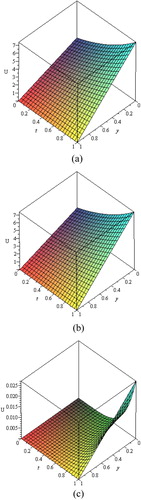
From Table 1, it is observed that the values of the approximate solution at different grid points obtained by the MHPM are similar to the values of the exact solution at the tenth term approximation.

Example 4.2

Next, consider the following two-dimensional fractional diffusion equation

(28) with the initial condition(29) By applying the aforesaid method, we get(30) Comparing the coefficients of like powers of p, we have(31) Therefore, the MHPM series solution is(32) If we set α = 1 in (28), we reproduce the solution of the problem as follows(33) This solution is equivalent to the exact solution in closed form(34) The numerical results for the exact solution (34) and the approximate solution (32) for α = 1 obtained by MHPM are shown in Fig. 2. It is observed from Fig. 2(a and b) that U(x, y, t) increases with the increase in both y and t when α = 1 and x = 1. It can be seen from the Fig. 2 that the solution obtained by the MHPM is nearly identical with the exact solution. It is to be noted that only the fourth order term of the MHPM was used in evaluating the approximate solutions for Fig. 2. It is evident that the efficiency of the present method can be dramatically enhanced by computing further terms of U(x, y, t) when the MHPM is used.

Figure 2 The surface shows the solution U(x, y, t) for Eqs. 28, 29 when α = 1 and x = 1: (a) Exact solution (34); (b) Approximate solution (32); (c) |U_ex − U_app|.

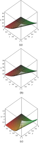
Table 1 Comparison study between the exact solution and approximate solution obtained by MHPM, when α = 1, x = 0.5 and t = 0.5.

y	Exact solution	Appr. solution	E10 (U) = |Uex − Uapp|
0	2.718281828	2.718281828	0
0.2	2.174625462	2.174625462	0
0.4	1.630969097	1.630969097	0
0.6	1.087312731	1.087312731	0
0.8	0.5436563656	0.5436563656	0
1.0	0	0	0

From Table 2, it is to be noted that the values of the approximate solution at different grid points obtained by the MHPM are close to the values of the exact solution with high accuracy at the tenth term approximation.

Example 4.3

Finally, consider the following three-dimensional fractional diffusion equation

(35) with the initial condition(36) By applying the aforesaid method, we get(37) Comparing the coefficients of like powers of p, we have(38) Therefore, the MHPM series solution is(39) If we take α = 1 in (35), we reproduce the solution of the problem as follows(40) This solution is equivalent to the exact solution in closed form(41) The numerical results for the exact solution (41) and the approximate solution (39) for α = 1 obtained by MHPM are shown in Fig. 3. It is observed from Fig. 3(a and b) that U(x, y, z, t) decreases with the increase in y when α = 1, x = 1 and z = 1. It can be seen from the Fig. 3 that the solution obtained by the MHPM is nearly identical with the exact solution. It is to be noted that only the fourth order term of the MHPM was used in evaluating the approximate solutions for Fig. 3. It is evident that the efficiency of the present method can be dramatically enhanced by computing further terms of U(x, y, z, t) when the MHPM is used.

Figure 3 The surface shows the solution U(x, y, z, t) for Eqs. 35, 36 when α = 1, x = 1 and z = 1: (a) Exact solution (41); (b) Approximate solution (39); (c) |U_ex − U_app|.

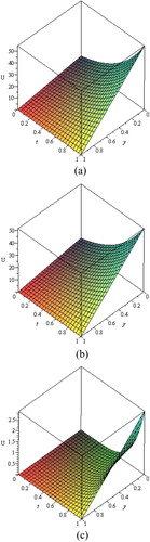
Table 2 Comparison study between exact solution and approximate solution obtained by MHPM, when α = 1, x = 0.5 and t = 0.5.

y	Exact solution	Appr. solution	E10 (U) = |Uex − Uapp|
0	4.481689070	4.481689029	4.1 × 10^−8
0.2	5.473947392	5.473947339	5.3 × 10^−8
0.4	6.685894442	6.685894379	6.3 × 10^−8
0.6	8.166169913	8.166169839	7.7 × 10^−8
0.8	9.974182455	9.974182362	9.3 × 10^−8
1.0	12.18249396	12.18249385	1.1 × 10^−7

From Table 3, it is observed that the values of the approximate solution at different grid points obtained by the MHPM are close to the values of the exact solution with high accuracy at the tenth term approximation.

Table 3 Comparison study of exact solution and approximate solution obtained by MHPM, when α = 1, x = 0.5, z = 0.5 and t = 0.5.

y	Exact Solution	Appr. Solution	E10 (U) = |Uex − Uapp|
0	7.389056099	7.389056023	7.6 × 10^−8
0.2	5.911244879	5.911244818	6.1 × 10^−8
0.4	4.433433659	4.433433614	4.5 × 10^−8
0.6	2.955622440	2.955622409	3.1 × 10^−8
0.8	1.477811220	1.477811205	1.5 × 10^−8
1.0	0	0	0

5 Concluding remarks

In this work, our main concern has been to study the two- and three-dimensional fractional diffusion equations. An approximation to the analytic solution for the range t > 0 was obtained by applying the MHPM with the help of the sumudu transform and symbolic calculations. The technique provides the solutions in terms of convergent series with easily computable components in a direct way without using linearization, perturbation or restrictive assumptions. Thus, it can be concluded that the MHPM is very powerful and efficient in finding analytical as well as numerical solutions for wide classes of fractional partial differential equations.

Acknowledgements

The authors are extending their heartfelt thanks to the reviewers for their valuable suggestions for the improvement of the article.

Notes

Peer review under responsibility of University of Bahrain.