Tri-prong scheme for regularized long wave equation

Peer review under responsibility of University of Bahrain.

Abstract

This paper witnesses the application of a tri-prong scheme comprising the well-known Variational Iteration (VIM), Adomian’s polynomials and an auxiliary parameter to obtain solutions of regularized long wave (RLW) equation in large domain. Computational work elucidates the solution procedure appropriately and comparison with results by the standard variational iteration method shows that the auxiliary parameter proves very effective to control the convergence region of approximate solutions.

Keywords:

• Regularized long wave equation
• Variational iteration method
• Adomian’s polynomials
• Auxiliary parameter

1 Introduction

Recently, lot of attention is being given to nonlinear sciences due to the fact that most of the physical phenomenons are nonlinear in nature. The regularized long wave (RLW) equation is one of the important partial differential equations of the nonlinear dispersive waves. Solitary waves are wave packet or pulses, which propagate in nonlinear dispersive media. Due to dynamical balance between the nonlinear and dispersive effects, these waves retain a stable wave form. The one-dimensional RLW equation is as follows:(1) with the physical initial conditionwhere γ > 0 is constant. This equation was first proposed by Peregrine in 1966 (Peregrine, 1966) as an alternative model to the KdV equation. The word “regularized” refers to the fact that the RLW equation has been studied extensively by Benjamin, Bona and Mahoney (Benjamin et al., 1972) and indeed, the equation is also referred to as the BBM equation. The RLW equation plays a major role in the study of non-linear dispersive waves (Abdulloev et al., 1976; Bona et al., 1985") because of its description of a larger number of important physical phenomena, such as shallow water waves and ion acoustic plasma waves. Experimental evidence suggests that this description breaks down if the amplitude of any wave exceeds about 0.28, as wave breaking is observed with water waves (Dogan, 2002).

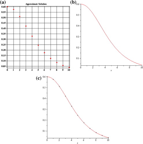
Figure 1d 4th- order approximation solution by present technique when h = 0.4476 in Example 4.1.

Figure 1e 4th-order approximation solution by standard VIM in Example 4.1.

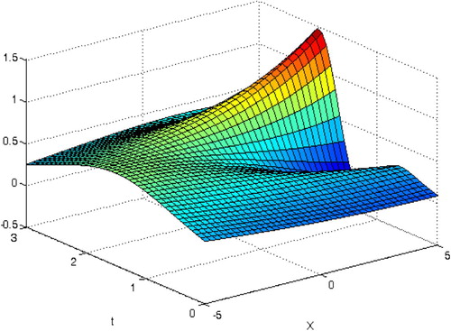
Figure 4 Error analysis of solution of Eq. (13)(13) by finite difference method.

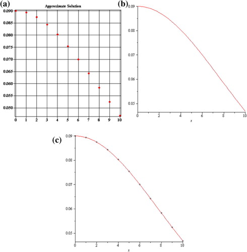
Figure 5a Absolute error for the 3rd-order approximation by standard VIM for u₃(x,t) in Example 4.3.

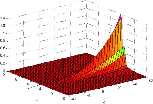
Figure 5b Absolute error for the 3rd-order approximation by present technique when h = 0.2712 in Example 4.3.

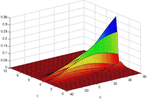
Figure 6 Error analysis of solution of Example 4.3 by finite difference method.

The RLW equation has solitary wave solutions similar to those of the KdV equation, and the interaction of solitary waves studied by Benjamin et al. (1972); Bona et al. (1980) suggested that the RLW wave interactions are inelastic, it was shown by Olver (1979) that the equation has three independent solution invariants. The possession of only a finite number of conservation conditions indicates that the equation is non-integrable and it is not amenable to attack by the IST method (Sloan, 1991). Since the analytical solution of the RLW equation is not very useful, the availability of accurate and efficient numerical methods is essential.

The numerical solution of the RLW equation has been considered by many authors. Peregrine used a finite-difference scheme to solve this equation, which is second-order in space and first-order in time (Peregrine, 1966). Bona and Pritchard applied the Runge–Kutta and predictor/corrector methods to obtain RLW equation (Bona et al., 1985). Various numerical studies have been reported based on the finite difference (Qianshun et al., 1995), pseudo-spectral (Gou and Cao, 1988), splitting (Jain et al., 1993) and Galerkin methods (Sanz-Serna and Christie, 1981). Gardner et al. used a least-squares technique with space linear finite elements to construct a numerical solution for this equation (Gardner et al., 1996). In addition, finite element method based on both quadratic and cubic B-spline finite elements within Galerkin’s method has been used for obtaining the solutions of the RLW equation by Gardner et al., 1995. Soliman and Raslan solved the RLW equation by using the collocation method with quadratic B-spline at the midpoint (Soliman and Raslan, 2001). Soliman and Hussein used the collocation method with septic spline to solve the RLW equation (Soliman and Hussien, 2005). Dong solved the RLW equation with the petrov-Galerkin method using quadratic B-spline finite elements (Dogan, 2001). Shokri and Dehghan used a mesh less method by the radial basis functions for numerical solution of the RLW equation (Shokri and Dehghan, 2010). Recently, semi-analytic methods have been used to solve the RLW equation. Some of these methods are the Adomian decomposition method (El-Danaf et al., 2005), homotopy analysis method (Rashidi et al., 2009), homotopy perturbation method (Inc and Uğurlu, 2007) and variational iteration method (Yusufoglu and Bekir, 2007).

In He, 1999, Ji-Huan He gave a very lucid as well as elementary discussion of the variational iteration method; the method was further developed by the originator himself (He, 2006, 2007; He et al., 2010"). The main property of the method is its flexibility and ability to obtain solutions of nonlinear equations accurately and conveniently (Noor and Mohyud-Din, 2008 ; Herişanu and Marinca, 2010; Yilmaz and Inc, 2010"). Also, there are many modifications of the variational iteration method, among which Herisanu and Marinca’s modification is much more attractive, where the variational iteration method is coupled with the least squares technology, and one iteration leads to ideal results (He, 2007). Yilmaz and Inc constructed a variational iteration algorithm, where an auxiliary parameter was introduced to adjust the convergence rate, but they did not give a general rule for the best choice of the auxiliary parameter (Yilmaz and Inc, 2010). This modified method was further developed by Hosseini et al. (2010a,b, 2012)"; Ghaneai et al. (2012) by introducing some profitable rules for optimal determination of the auxiliary parameter. It is to be highlighted that Abbasbandy (2007a,b)" introduced Adomian’s polynomials in the traditional VIM for solving quadratic Riccati differential and Klein-Gordon equations and subsequently Noor and Mohyud-Din (2008) for solving singular and nonsingular initial and boundary value problems. Ref., (Biswas and Zerrad, 2007; Biswas, 2010; Biswas and Kara, 2011; Girgis et al., 2010; Girgis and Biswas, 2011; Antonova and Biswas, 2009; Girgis and Biswas, 2010; Labidi et al., 2012; Kirshnan et al., 2011; Kirshnan et al., 2012") also discuss regularized long wave equation in detail. Recently, Hosseini et al. (2011) made an elegant coupling of Auxiliary parameter, Adomian’s polynomials and correction functional to solve nonlinear problems. Inspired and motivated by the ongoing research in this area, we apply the tri-prong algorithm (Hosseini et al., 2011) which is obtained by inserting Adomian’s polynomials in the correction functional having auxiliary parameter to find approximate solutions of RLW equation.

2 Variational Iteration Method (VIM)

Hereby, we briefly recapitulate the standard solution procedure of the variational iteration method. Consider the following functional equation:(2) where L is the highest order derivative that is assumed to be easily invertible, R is a linear differential operator of order less than L, Nu represents the nonlinear terms, and g is the source term. The basic characteristic of He’s method is to construct a correction functional for Eq. (2)(2) , which reads:(3) where λ is a Lagrange multiplier which can be identified optimally via variational theory, u_n is the nth approximate solution, and denotes a restricted variation, i.e., . After identification of the multiplier, a variational iteration algorithm is constructed, an exact solution can be achieved when n tends to infinity:(4) In summary, we have the following variational iteration formula for (2)(2) :(5)

3 Auxiliary parameter in variational iteration algorithm

An unknown auxiliary parameter h can be inserted into the variational iteration algorithm, Eq. (5)(5) :(6) It should be emphasized that u_n(x,h),n ⩾ 1 can be computed by symbolic computation software such as Maple or Mathematica. The approximate solutions u_n(x,h),n ⩾ 1 contain the auxiliary parameter h. The validity of the method is based on such an assumption that the approximation u_n(x,h),n ⩾ 0 converges to the exact solution. It is the auxiliary parameter h that ensures that the assumption can be satisfied. In general, by means of the error of norm two of the residual function, it is straightforward to choose a proper value of h which ensures that the approximate solutions are convergent (Hosseini et al., 2010a,b, 2012; Ghaneai et al., 2012"). In fact, the proposed technology is very simple, easier to implement and is able to approximate the solution more accurately in a large solution domain.

4 Numerical examples

To elucidate the solution procedure, three examples are given.

Example 4.1

Consider the following RLW equation (Rashidi et al., 2009):(7) which admits the solution u(x,t) = 3α sech²(β [x − (1 + α)t]), where α > 0 is constant and . Take (x,t) ∈  [ − 5,5] × [0,3]. According to the traditional Variational Iteration Method, we get(8) Now, using algorithm defined in Hosseini et al. (2010a,b, 2011, 2012), Ghaneai et al. (2012)", we have the following correction functional using Adomian’s polynomials:(9) where A_n are the so-called Adomian’s polynomials. Now, beginning with u₀(x,t) = u(x,0) = 3α sech²(βx) and α = 0.2, we stop the solution procedure at u₄(x,t). Fig. 1a, is the absolute error of u₄(x,t) for (x,t) ∈  [ − 5,5] × [0,3], showing that the solution u₄(x,t) is not valid for large values of x and t, of course, the accuracy can be improved if the iteration procedure continues and the exact solution can be obtained when n tends to infinity. Now, using the recursive scheme (6)(6) , we have:and in general,(10)

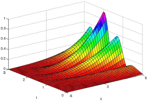
Figure 1a Absolute error for the 4th-order approximation by standard VIM in Example 4.1.

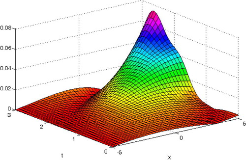
In order to find a proper value of h for the approximate solutions (9)(9) , we define the following residual function,(11) and the following error of norm two of the residual function,(12) Here, we apply numerical integration to calculate the approximate e₄ (h). For obtaining an optimal value of h, we choose the minimum point of the error of norm two of residual function (12)(12) . The minimum point of e₄(h), as h = 0.4476, is obtained by using Maple software. By substituting h = 0.4476 in u₄(x,t,h), the absolute error of the 4th-order approximation of the proposed method reduces remarkably, as shown in Fig. 1b.

Figure 1b Absolute error for the 4th-order approximation by present technique when h = 0.4476 in Example 4.1.

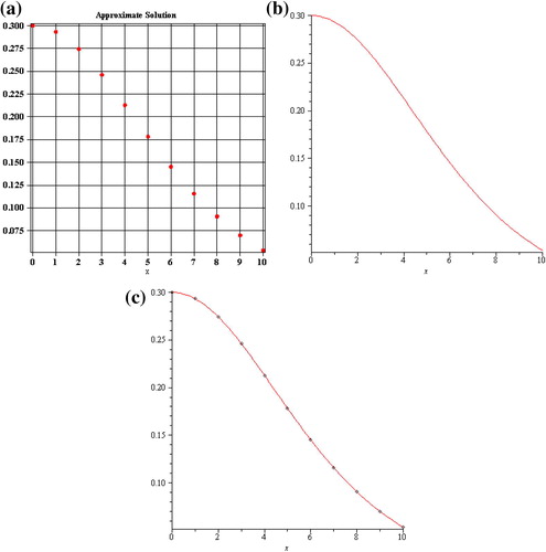
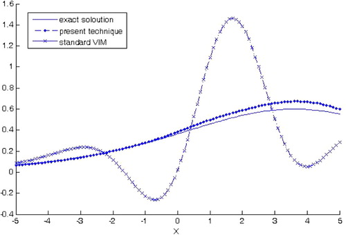
Fig. 1c shows the exact solution, and Figs. 1d and 1e show the 4th- approximation solution by standard VIM and the present technique, respectively. In addition, the plot of numerical results for u₄(x,t) by standard VIM and present technique in comparison with the exact solution at t = 3 s, is shown in Fig. 1f. The results show the high efficiency of the proposed method in this example.

Figure 1c Exact solution for Example 4.1.

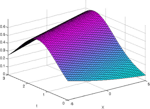
Figure 1f The plot of numerical results for u₄(x,t) by standard VIM and present technique in comparison with the exact solution at t = 3 s, in Example 4.1.

Using forward difference (Liszka and Orkisz, 1980) for time derivative and center difference for x direction we get the required formThe initial and boundary conditions are given asLet us denote This numerical scheme has traction error of O(k) + O(h²) which is similar to Kutluay and Esen, 2006. Since the stability parameter k/h² depends not only on the form of the proposed finite difference scheme but also generally upon the solution u(x,t) being obtained, the complications and difficulties may arise in the analysis of stability. Let us take m = 5 and n = 5 where m and n are number of meshes in x and t directions where x = ih and t = jk. According to this and . Taking i = 1, 2, 3, 4 and j = 0, 1, 2, 3, 4, 5. Using initial and boundary data we can have tri diagonal matrix of the form for j = 0 and i = 1, 2, 3, 4.After solving we have the following error table.

Table

x	Exact solution	Approx. sol. k = 0.6	Approx. sol. k = 0.1	Approx. sol. k = 0.01
0.0	0.600000	0.600000	0.600000	0.600000
2.0	0.510146	0.511240	0.510120	0.510146
4.0	0.328115	0.310154	0.328784	0.328114
6.0	0.175583	0.174125	0.175142	0.175581
8.0	0.084973	0.084875	0.084453	0.084970
10.0	0.039146	0.034125	0.039145	0.039141

Example 4.2

Consider the following RLW equation (Yusufoglu and Bekir, 2007):(13) It is easy to verify that u(x,t) = 3c sech²(p(x − vt − x₀)), where and c is constant. We take the solution domain as (x,t) ∈ [ − 25,25] ×  [0,50]. Similarly, the absolute error of u₃(x,t) for (x,t) ∈ [ − 25,25] × [0,50], c = 0.03, γ = 1, and x₀  = 0 tends to be very large when time tends to 50, as illustrated in Fig. 2(a).

Figure 2 Error analysis of solution of Eq. (7)(7) by finite difference method.

According to the traditional Variational Iteration Method, we get(14) Now, using algorithm defined in Hosseini et al. (2010a,b, 2011, 2012), Ghaneai et al. (2012)", we have the following correction functional using Adomian’s polynomials:(15) where A_n are the so-called Adomian’s polynomials. Now, using the iteration formulation (6)(6) , we successively haveand in general,We define the following residual function,and the following error of norm two of the residual function,clearly, suitable value of h is the global minimum point of e₃ (h) which we obtain as h = 0.025 using Maple software. The absolute error of 3rd-order approximation of the proposed method in the solution domain (x,t) ∈ [ − 25,25] × [0,50], is given in Fig. 2(b), the accuracy is remarkably improved by the optimal choice of h.

After solving by FDM, we have the following error table.

Table

x	Exact solution	Approx. sol. k = 0.6	Approx. sol. k = 0.1	Approx. sol. k = 0.01
0.0	0.090000	0.090000	0.090000	0.090000
5.0	0.075418	0.075210	0.075124	0.075411
10.0	0.046803	0.046421	0.046812	0.046812
15.0	0.023980	0.023142	0.023921	0.023940
20.0	0.011112	0.011242	0.011231	0.011121
25.0	0.004912	0.001420	0.004221	0.004899

Example 4.3

Consider the RLW Eq. (13)(13) , in a third numerical experiment, we take c = 0.1, γ = 1, x₀ = 0 through the interval [ − 40,60] ×  [0,10]. According to the standard VIM, we have the following variational iteration formula:Beginning with , we calculate the approximate solution till u₃(x,t). The absolute error is shown in Fig. 3a, it is obvious that the same problem keeps unchanged. Similarly, by the iteration algorithm (6)(6) , we haveand in generalWe define the residual function of u₃(x,t) as,(16)

Figure 3a Absolute error for the 3rd-order approximation by standard VIM for u₃(x,t) in Example 4.2.

For obtaining an optimal value of h, we choose the global minimum point of the error of norm two of residual function (16)(16) :thus we select h = 0.2712. The absolute error of 3rd-order approximation of the proposed method in the solution domain (x,t) ∈  [ − 25,25] × [0,50], is given in Fig. 3b, the accuracy is remarkably improved by the optimal choice of h (see Figs. 5a and 5b).

Figure 3b Absolute error for the 3rd-order approximation by present technique when h = 0.025 in Example 4.2.

After solving by FDM, we have the following error table.

Table

x	Exact solution	Approx. sol. k = 0.6	Approx. sol. k = 0.1	Approx. sol. k = 0.01
0.0	0.300000	0.300000	0.300000	0.300000
5.0	0.178117	0.176312	0.178112	0.178117
10.0	0.053475	0.052568	0.053445	0.053474
15.0	0.012753	0.011245	0.012714	0.012752
20.0	0.002872	0.005483	0.002845	0.002871
25.0	0.000638	0.001254	0.000636	0.000629
30.0	0.000141	0.002133	0.000147	0.000148

By using the transformation ξ = kx + ωt, and sech method of the Eq. (1)(1) , we getConsider the trial solution u(ξ) = a₀ + a₁ sech(ξ) + a₂ sech²(ξ), then follow the methodology given in Davodi et al., 2009, we have the following solution setTheir corresponding solution is(16) For and γ = 1, Eq. (16)(16) becomes the solution to Eq. (7)(7) , for k = 0.0853320186 and γ = 1, Eq. (16)(16) becomes the solution to Eq. (13)(13) , and for k = 0.1507556723, and γ = 1, Eq. 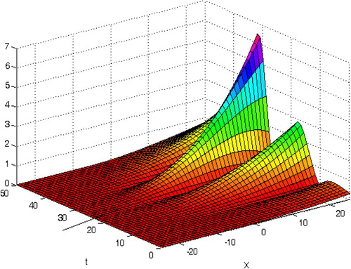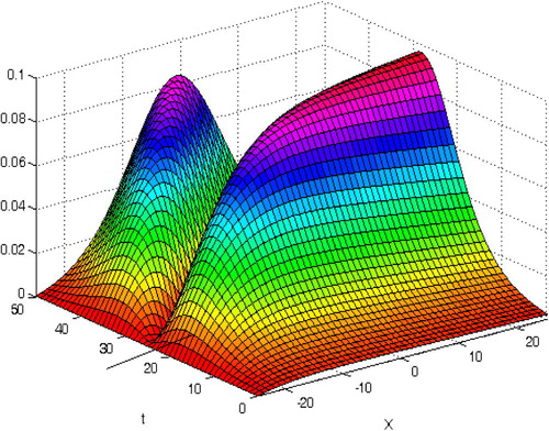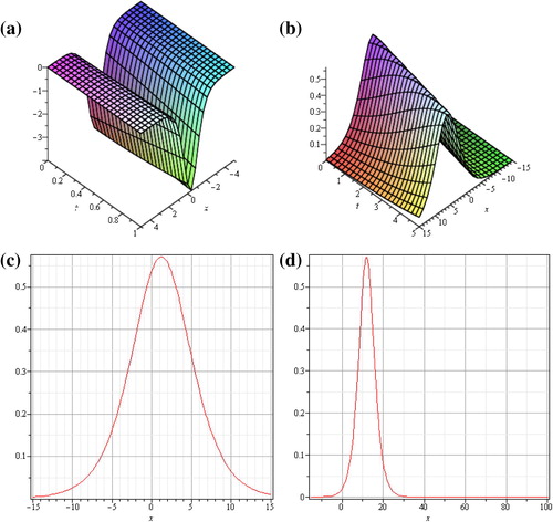(16)(16) becomes the solution to Example 3.3. Their graphical representation is give in Fig. 7 .

Figure 7 Travelling wave solution of Eq. (1)(1) for different values of parameters.

5 Conclusion

The present technique provides a simple way to adjust and control the convergence region of approximate solution of regularized long wave (RLW) equation for any values of t and x. An optimal auxiliary parameter can be determined by the error of norm two of the residual function. The obtained results are compared with numerical method “Finite Difference Method”. Tables 1-3 represent the error table for different values of k and Figs. 2,4,6 represent the error analysis. Sech method was also applied hence different values of k in their solution are identical to the proposed algorithms and Fig. 7 represents the physical interpretation in 2D and 3D of Eq. (1)(1) , this graph shows solitary wave solution, i. e., as t increases the graph travels at a constant speed and maintains its shape. Numerical results and graphical representations explicitly reveal the complete reliability of proposed method. It needs to be highlighted that the proposed variational iteration algorithm involving an auxiliary parameter is particularly suitable for inverse problems and differential-difference equations with large domain.

Notes

Peer review under responsibility of University of Bahrain.