An efficient numerical method for the modified regularized long wave equation using Fourier spectral method

Peer review under responsibility of University of Bahrain.

Abstract

The modified regularized long wave (MRLW) equation is numerically solved using Fourier spectral collection method. The MRLW equation is discretized in space variable by the Fourier spectral method and Leap-Frog method for time dependence. To validate the efficiency, accuracy and simplicity of the used method, four cases study are solved. The single soliton wave motion, interaction of two solitary waves, interaction of three solitary waves and a Maxwellian initial condition pulse are studied. The and error norms are computed for the motion of single solitary waves. To determine the conservation properties of the MRLW equation three invariants of motion are evaluated for all test problems.

Keywords:

• MRLW equation
• Fourier spectral method
• Fast Fourier transform
• Leap-Frog method
• Solitary waves

1 Introduction

The regularized long wave (RLW) equation

(1.1) where is a positive constant, is a nonlinear evolution equation, which was originally introduced by Peregrine (1966) in describing the behavior of an undular bore and studied later by Benjamin et al. (1972). This equation plays an important role in describing physical phenomena in various disciplines, such as the nonlinear transverse waves in shallow water, ion-acoustic waves in plasma, magneto–hydrodynamics waves in plasma, longitudinal dispersive waves in elastic rods, and pressure waves in liquid’s gas bubbles. Many numerical methods for the RLW equation have been proposed, such as the finite element method, Galerkin method, collocation methods with quadratic B-splines, an explicit multistep method, finite difference methods and Fourier Leap-Frog method (Liu et al., 2013; Saka and Dag, 2008; Soliman and Raslan, 2001; Mei and Chen, 2012; Lin et al., 2007; Hassan and Saleh, 2010). The RLW equation is a special case of the generalized regularized long wave (GRLW) equation(1.2) where and are positive constants and is a positive integer. Various numerical techniques have been used for the solution of the GRLW equation as (Mohammadi and Mokhtari, 2011; Kaya, 2004; Roshan, 2012; Hammad and El-Azab, 2015; Zeybek and Karakoç, 2016). The modified regularized long wave equation (MRLW) is a special form of GRLW Eq. (1.2)(1.2) and it plays a very important role at the modeling of the nonlinear, dispersive media being modeled feature small-amplitude, long-wave length disturbances. The MRLW equation was also solved using various numerical methods such as, a Galerkin finite element method, a spline method, the Adomian decomposition method, a collocation method with cubic B-splines, finite difference scheme, meshless kernel based method of lines, B-spline finite elements, mixed Galerkin finite element methods, Tri-prong scheme, homotopy perturbation method and He’s variational iteration method as Mei et al. (2014), Raslan and EL-Danaf (2010), Raslan and Hassan (2009), Khalifa et al. (2007, 2008a,b), Dereli (2012), Gardner et al. (1997), Gao and Mei (2015), Hosseini et al. (2016), Achouri and Omrani (2010), Labidi and Omrani (2011). Discretization using finite differences in time and spectral methods in space has proved to be efficient in solving numerically non-linear partial differential equations (PDE) describing wave propagation. The combined schemes have been applied efficiently to analyze unidirectional solitary wave propagation in one dimension Korteweg de Vries (KdV) equation as Fornberg (1996), Fornberg and Whitham (1987), Hassan and Saleh (2013). The combination of spectral methods and finite differences is applied to the Boussinesq type which admits bidirectional wave propagation as Hassan (2010), Borluk and Muslu (2015). The numerical solution for the modified equal width wave (MEW) equation is presented using Fourier spectral method by Hassan (2016). Different analytical and numerical methods are used to solve differential equations as Atangana and Cloot (2013), Atangana (2016), Semary and Hassan (2016), El-Borai et al. (2017). In this study, the combination of Fourier spectral method in space and leap frog in time is applied to the modified regularized long wave equation (MRLW) equation. Consider the MRLW equation(1.3) where the subscripts x and t denote differentiation, is considered with the boundary conditions as . In this study, boundary conditions are chosen from(1.4) and the initial condition(1.5) where function will be chosen later. The numerical solution of the MRLW equation is investigated using the Fourier Leap-Frog methods. The used method is validated by studying the motion of a single solitary wave, development of interaction of two positive solitary waves, development of three positive solitary waves interaction and a Maxwellian initial condition pulse is then studied.

2 Analysis of the numerical scheme

A numerical method is developed for the periodic initial value problem in which u is a prescribed function of x at t = 0 and the solution is periodic in x outside a basic interval . Interval may be chosen large enough so the boundaries do not affect the propagation of solitary waves. The Eq. (1.1)(1.1) can be written as

(2.6) where(2.7) For ease of presentation the spatial period [a, b] is normalized to [0, 2π] using the transformation , where . is transformed into Fourier space with respect to x, and derivatives (or other operators) with respect to x. This operation can be done with the Fast Fourier transform (FFT). Applying the inverse Fourier transform . Then, we need to discretize the results equations. For any integer consider The solution is transformed into the discrete Fourier space as(2.8) And the inverse formula is(2.9) After all the previous mathematical operations to Eqs. (2.7)(2.7) and (2.6)(2.6) , and then reducing the resulting equation to the equations(2.10) (2.11) Letting .

The ordinary differential equation (2.11)(2.11) can be written in the vector form(2.12) where defines the right hand side of (2.11)(2.11) . The Leap Frog method (two-step scheme) is given as(2.13) is used to solve the resulting ordinary differential equation (2.12)(2.12) in time. Use the Leap-Frog scheme to advance in time to obtain

Finally, we find the approximate solution using the inverse Fourier transform (2.9)(2.9) . The Leap-Frog needs two levels of initial value; we begin with to get from (2.10)(2.10) , then(2.14) (2.15) Then evaluate the second level of initial solution by using a higher-order one-step method, for example, a fourth-order Runge–Kutta method (RK4), then substitute in (2.14)(2.14) as(2.16) to obtain . Thus, Eq. (2.12)(2.12) become(2.17) By substituting and in (2.17)(2.17) to evaluate then substitute in (2.16)(2.16) to evaluate , so we have and , then substitute in (2.17)(2.17) to evaluate , and evaluate from (2.16)(2.16) and so on, until we evaluate at time . We use FFT routines in MATLAB (i.e., fft and ifft) to calculate Fourier transform and the inverse Fourier transform.

3 The validity of the numerical scheme

To check the efficiency and accuracy of the used numerical method, many test problems will be considered: propagation of single soliton and collision of two and three solitons at different time levels. Finally, we investigate the development of the Maxwellian initial condition into solitary waves. Due to the existence of the analytical solution in the first test problem, the error between analytical and numerical solutions can be calculated using and norms defined by

(3.18) The conservation properties of the MEW equation will be examined by calculating the following three invariants, given as Khalifa et al. (2008a) which respectively correspond to mass, momentum, and energy.(3.19) These invariants are used to check the conservative properties of a numerical method, especially for problems without an analytical solution and during collision of solitons. The integrals are approximated by sums to obtain the numerically values of invariants in (3.19)(3.19) at the finite domain as follows:(3.20)

3.1 Application 1: single solitary wave

The analytic solution of the MRLW equation is given by Gardner et al. (1997):(3.21) with boundary condition as , where , and c are real constants, and the initial condition given as(3.22) The analytical values of the three invariants are(3.23) To compare with some previous results, two problems are studied for single solitary wave.

Problem 1

The parameters are chosen as , , , , and in time period . The analytical values for the invariants are , and . Invariants and error norms for a single solitary wave at different values of time are presented in Table 1. The motion of single solitary waves is shown in Fig. 1. The program is run up to time over the solution domain. Initially at the peak position of solitary wave was positioned at with amplitude 0.22360680 and at the end of time location of peak position of the wave reached to with amplitude 0.22359503. It is clear from Fig. 1 that the single solitary wave moved to the right with the preserved amplitude and shape. As it is seen from Table 2, the error norms decrease (halved) when N increases (doubled) and numerical invariants are closed to the analytical values when N increases and its values remain almost constant when compared with analytical values of invariants. Calculated numerical results are very satisfactorily. The comparison between the results obtained by the present method with those in the other studies is also documented in Table 2. The obtained results by the present method are accurate compared with the other methods and also the used method is simple.

Problem 2

In the second problem, the parameters are chosen as , , , , and in the time period . The analytical values for the invariants are , and . Invariants and error norms for a single solitary wave at different values of time are presented in Table 3. The motion of single solitary waves is plotted in Fig. 2. The program is run up to time over the solution domain. Initially at the peak position of solitary wave was positioned at with amplitude 0.54772256 and at the end of time location of peak position of the wave reached to with amplitude 0.54753484. It is clear from Fig. 2 that the single solitary wave moved to the right with the preserved amplitude and shape. As it is seen from Table 4, the results are accurate like that in problem 1.

Figure 1 (a) Motion of the single solitary wave at different values of t, and (b) error distributions at with and .

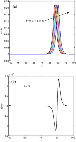
Figure 2 (a) Motion of the single solitary wave at different values of t, and (b) error distributions at with and .

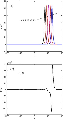
Table 1 Invariants and error norms for the single soliton with , , and .

0	3.217600191	0.465311294	0.007990311	0.0000000	0.0000000
2	3.217600191	0.465311294	0.007990311	0.1670832	0.0467942
4	3.217600191	0.465311294	0.007990311	0.2448388	0.0684808
6	3.217600191	0.465311294	0.007990311	0.2336465	0.0651000
8	3.217600191	0.465311294	0.007990311	0.3116369	0.0871898
10	3.217600191	0.465311294	0.007990311	0.4787285	0.1347674

Table 2 Invariants and error norms for the single soliton with at different values of N at t = 10 and comparison with different methods.

N
256	1	0.001	3.206599616	0.463769956	0.007913129	3.209604	0.897132
512	1	0.001	3.212887075	0.464650699	0.007957254	1.648256	0.459176
1024	1	0.001	3.216030800	0.465091092	0.007979295	0.868371	0.241774
2048	0.1	0.001	3.217600191	0.465311294	0.007990311	0.478729	0.134767
4096	0.1	0.001	3.218388594	0.465421396	0.007995817	0.283909	0.080088
8192	0.1	0.001	3.218781559	0.465476447	0.007998570	0.186614	0.052793
Raslan and Hassan (2009)
Quad.	0.2	0.2	3.215653	0.4655665	0.008004883	0.199288	0.481156
Cubic	0.2	0.2	3.215189	0.4655136	0.007999173	0.453811	0.625887

Table 3 Invariants and error norms for the single soliton with , , and .

0	3.580217732	1.344513519	0.153554106	0.0000000	0.0000000
5	3.580217732	1.344513519	0.153554106	0.6476041	0.2724080
10	3.580217732	1.344513519	0.153554106	1.6894359	0.7287846
15	3.580217732	1.344513519	0.153554106	2.3600926	1.0236940
20	3.580217732	1.344513519	0.153554106	2.6423750	1.1493109

Table 4 Invariants and error norms for the single soliton with at different values of N at t = 10 and comparison with different methods.

N
256	1	0.001	3.567974713	1.340574276	0.152370272	21.103660	8.943814
512	1	0.001	3.574970715	1.342824656	0.153046586	10.552528	4.374456
1024	1	0.001	3.578468719	1.343950177	0.153384534	5.272343	2.198671
2048	0.1	0.001	3.580217732	1.344513519	0.153554106	2.642375	1.149311
4096	0.1	0.001	3.581092236	1.344794977	0.153638566	1.321486	0.574767
8192	0.1	0.001	3.581529488	1.344935710	0.153680791	0.660977	0.287463
Khalifa et al. (2008b)
	0.2	0.025	3.58197	1.34508	0.153723	0.606885	0.296650

3.2 Application 2: interaction of two solitary waves

Secondly, the interaction of two positive solitary waves is studied by using the initial condition given by the linear sum of two separate solitary waves of various amplitudes,(3.24) where , and () are arbitrary constants. The analytical values for the conservation laws in this case have the following form:(3.25) In this case study, parameters are taken as , , , , , and . These parameters provide solitary waves of magnitudes about 2 and 1 at and their peaks are positioned at and . The initial function was placed with the larger wave to the left of the smaller one as seen in the Fig. 3a. Both waves move to the right with velocities dependent upon their magnitudes. According to Fig. 3, the larger wave catches up with the smaller wave at about , the overlapping process continues until , then two solitary waves emerge from the interaction and resume their former shapes and amplitudes. At , the magnitude of the smaller wave is 0.996049 on reaching position , and of the larger wave 1.999735 having the position , so that the difference in amplitudes is 0.003951 for the smaller wave and 0.000265 for the larger wave. The analytic invariants are , and . Table 5 displays the values of the invariants obtained by the present method. It is observed that the obtained values of the invariants remain almost constant during the computer run and close to analytic values.

Figure 3 Interaction of two solitary waves at different t.

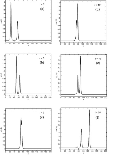
Table 5 Invariants for interaction of two solitary waves at different times.

0	11.462098207	14.624889848	22.866503875
2	11.462098207	14.624770155	22.866030604
4	11.462098207	14.624770137	22.866030613
6	11.462098207	14.624773601	22.866044720
8	11.462098207	14.624760431	22.866010568
10	11.462098207	14.624759478	22.866005516
12	11.462098207	14.624770339	22.866030712
14	11.462098207	14.624770321	22.866030942
16	11.462098207	14.624770256	22.866030937
18	11.462098207	14.624770230	22.866030930
20	11.462098207	14.624770217	22.866030928

3.3 Application 3: interaction of three solitary waves

In this section, the interaction of three solitary waves is studied with the initial conditions given by a linear sum of three separate solitary waves of various amplitudes:(3.26) where , and () are arbitrary constant. The analytical values for the conservation laws in this case have the following form:(3.27) In this case, parameters are chosen as , , , , , , , and . Solitary wave having the largest amplitude is located to the left of the smaller ones. As is well known, solitary waves with larger amplitudes have a greater velocity than those with smaller amplitudes. Consequently, as time goes on the larger two solitary waves catch up with the smaller one, the overlapping process of the three solitary waves continues while the larger solitary waves have overtaken the smaller ones. Plot of the three solitary waves is depicted at various times in Fig. 4. At , the amplitudes of the smaller waves are 0.481476 at the point and 1.014965 at the point , whereas the amplitude of the larger one is 1.997794 at the point , so that the difference in amplitudes is 0.018524, 0.014965 and 0.002206. The analytic invariants are , and . Table 6 displays the values of the invariants obtained by the present method. It is observed that the obtained values of the invariants remain almost constant during the computer run and close to analytic values.

Figure 4 Interaction of three solitary waves at different t.

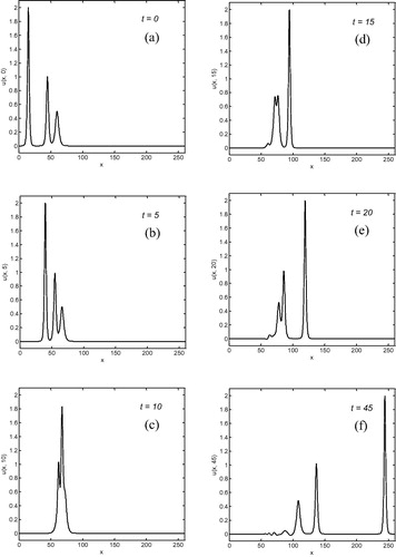
Table 6 Invariants for interaction of three solitary waves at different times.

0	14.972784239	15.8326196890	22.994076591
5	14.972784239	15.832499932	22.993603647
10	14.972784239	15.832470138	22.993546007
15	14.972784239	15.832498462	22.993602081
20	14.972784239	15.832499481	22.993602500
25	14.972784239	15.832499798	22.993602613
30	14.972784239	15.832499841	22.993602629
35	14.972784239	15.832499844	22.993602632
40	14.972784239	15.832499845	22.993602648
45	14.972784239	15.832500050	22.993603470

3.4 Application 4: the Maxwellian initial condition

Finally, the evolution of solitary waves is studied by using the Maxwellian initial condition(3.28) with boundary condition(3.29) As it is known, Maxwellian initial condition the behavior of the solution depends on the values of μ. We choose various values of as , and .

Calculated numerical invariants at different values of t for different values of μ are shown in Table 7 and it is seen that calculated invariant values are satisfactorily constant and close to the other solutions like Khalifa et al. (2008b) of invariants. The development of the Maxwellian initial condition is shown in Fig. 5 with different values of μ, respectively. The smaller there is, the more the number of solitary waves will form. For , it is observed that a single solitary wave is occurred, however, as the value of μ is reduced then the number of wave increases.

Figure 5 Maxwellian initial condition with different values and .

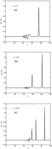
Table 7 Invariants for Maxwellian initial condition at different values of μ.

t	μ
0	0.1	1.771588395	1.378094808	0.760401557
3		1.771588395	1.378097446	0.760398361
6		1.771588395	1.378097446	0.760398344
9		1.771588395	1.378097416	0.760398351
12		1.771588395	1.378097415	0.760398352
15		1.771588395	1.378097455	0.760398333
		Khalifa et al. (2008b)
15		1.77247	1.37764	0.762126
0	0.04	1.771588395	1.302859224	0.835637141
3		1.771588395	1.302883963	0.835651071
6		1.771588395	1.302883968	0.835651065
9		1.771588395	1.302883951	0.835651074
12		1.771588395	1.302883952	0.835651071
15		1.771588395	1.302883953	0.835651071
		Khalifa et al. (2008b)
15		1.77254	1.30074	0.840643
0	0.015	1.771588395	1.271511064	0.866985301
3		1.771588395	1.271600511	0.867067547
6		1.771588395	1.271600614	0.867067541
9		1.771588395	1.271600621	0.867067539
12		1.771588395	1.271600623	0.867067541
15		1.771588395	1.271600623	0.867067541
		Khalifa et al. (2008b)
15		1.77303	1.26706	0.885111

4 Conclusion

The combination between Fourier spectral method and leap frog method has been applied to obtain the numerical solution of the modified regularized long wave equation (MRLW). The accuracy, efficiency and the simplicity of the present scheme were verified by four numerical applications: the motion of a single solitary wave and its accuracy was shown by calculating error norms L₂ and L_∞, the interaction of two solitary waves, the interaction of three solitary waves, and development of the Maxwellian initial condition pulse is then studied at different values of μ. This scheme numerically satisfies the conservation laws of mass, momentum, and energy. The obtained results show that the present method is a remarkably successful numerical method and efficiently applied to MRLW and other types of non-linear partial differential problems.

Notes

Peer review under responsibility of University of Bahrain.