A computational method based on hybrid of Bernstein and block-pulse functions for solving linear fuzzy Fredholm integral equations system

Peer review under responsibility of Taibah University.

Abstract

This paper deals with the solutions of linear fuzzy Fredholm integral equation systems by using a combination of Bernstein and block-pulse functions on the interval [0, 1), that is called hybrid functions. Moreover, the existence of the solution and convergence of the proposed method is proved. Finally, illustrative examples are included in order to demonstrate the accuracy and the convergence of this method.

Keywords:

• Fuzzy number
• Fredholm fuzzy integral equation system
• Block-pulse functions
• Bernstein polynomials
• Hybrid functions

1 Introduction

The integral equations have been one of the principal tools in various areas of applied mathematics, physics and engineering. Many different basic functions have been used to estimate the solution of integral equations, such as orthonormal bases and wavelets [1]. In recent years, the different kinds of hybrid functions are developing such as the hybrid functions consisting of the combination of block-pulse functions with Chebyshev polynomials [2–4] or Legendre polynomials [5–7].

Table 1 The maximum error of $({\underset{\_}{u}}_1(x,r),{\overline{u}}_1(x,r))$ and $({\underset{\_}{u}}_2(x,r),{\overline{u}}_2(x,r))$ of Example 2 for N = 2 and M = 3.

r	Maximum error	Maximum error	Maximum error	Maximum error
	${\underset{\_}{u}}_1(x,r)$ for x = 0.7	${\overline{u}}_1(x,r)$ for x = 0.7	${\underset{\_}{u}}_2(x,r)$ for x = 0	${\overline{u}}_2(x,r)$ for x = 0
0	0.000000000000000e−000	5.581971063151059e−007	0.000000000000000e−000	6.875888106383510e−007
0.1	3.478479890239861e−008	5.302872629897593e−007	3.437944034943679e−008	6.532093702993268e−007
0.2	6.956959780479721e−008	5.023773930190600e−007	6.875888072524483e−008	6.188299299600647e−007
0.3	1.043543967904625e−007	4.744675052847924e−007	1.031383211480264e−007	5.844504906316186e−007
0.4	1.391391957206167e−007	4.465576619594458e−007	1.375177616603767e−007	5.500710502767602e−007
0.5	1.739239947617932e−007	4.186478097523150e−007	1.718972022606014e−007	5.156916087732666e−007
0.6	2.087087935809251e−007	3.907379664269683e−007	2.062766428703681e−007	4.813121684305200e−007
0.7	2.434935928441462e−007	3.628281053380533e−007	2.406560835744032e−007	4.469327280579720e−007
0.8	2.782783921073673e−007	3.349182531309225e−007	2.750355247183462e−007	4.125532871021380e−007
0.9	3.130631913705884e−007	3.070084009237917e−007	3.094149656558945e−007	3.781738464660841e−007

Table 2 The maximum error of $({\underset{\_}{u}}_1(x,r),{\overline{u}}_1(x,r))$ and $({\underset{\_}{u}}_2(x,r),{\overline{u}}_2(x,r))$ of Example 2 for N = 2 and M = 6.

r	Maximum error	Maximum error	Maximum error	Maximum error
	${\underset{\_}{u}}_1(x,r)$ for x = 0.7	${\overline{u}}_1(x,r)$ for x = 0.7	${\underset{\_}{u}}_2(x,r)$ for x = 0	${\overline{u}}_2(x,r)$ for x = 0
0	0.000000000000000e−000	4.871125725003367e−010	0.000000000000000e−000	6.000348828916202e−010
0.1	2.794883768864054e−011	4.627676020163563e−010	3.000152563707726e−011	5.700333704957393e−010
0.2	5.589767537728108e−011	4.383959861797848e−010	6.000308491738160e−011	5.400318577891694e−010
0.3	8.384659633264846e−011	4.140243703432134e−010	9.000467442936249e−011	5.100310228567855e−010
0.4	1.117955727991671e−010	3.896793998592329e−010	1.200063822735537e−010	4.800294923041667e−010
0.5	1.397444382433832e−010	3.653521929436465e−010	1.500077388694177e−010	4.500269566720672e−010
0.6	1.676931926652969e−010	3.410072224596661e−010	1.800095704249799e−010	4.200254107915129e−010
0.7	1.956423911764205e−010	3.166444884072917e−010	2.100115502889910e−010	3.900238158659891e−010
0.8	2.235918117321489e−010	2.922906361391142e−010	2.400140680189778e−010	3.600217853764320e−010
0.9	2.515410102432725e−010	2.679367838709368e−010	2.700162701726235e−010	3.300199876615984e−010

The concept of fuzzy integral that was initiated by Dubois and Prade [8] and investigated by Goetschel and Voxman [9], Kaleva [10], Nanda [11] and others, attracted growing interest, in particular in relation to fuzzy control. There are several research papers about obtaining the numerical integration of fuzzy-valued functions and solving fuzzy Volterra and Fredholm integral equations, for example, the authors used Bernstein polynomials [12], Lagrange interpolation [13], divided and finite differences [14], Legendre wavelets [15], predictor–corrector procedures [16] and Taylor expansion [17] for solving fuzzy integral equations.

In this paper, we use a simple base, a combination of block-pulse functions on [0, 1) and Bernstein polynomials to solve linear Fredholm fuzzy integral equation systems. This paper is organized as follows. In Section 2, hybrid functions of block-pulse and Bernstein functions and its properties are introduced. In Section 3, we review some elementary concepts of the fuzzy calculus. In Section 4, fuzzy system of Fredholm integral equation is introduced. In Section 5, we prove the existence of the solution for systems of linear fuzzy Fredholm integral equations. In Section 6, we use the presented functions for approximating the solution of these systems. Convergence analysis of the presented method is discussed in Section 7. Section 8 includes two numerical examples for the proposed method. Finally, Section 9 gives our concluding remarks.

2 Properties of hybrid functions

2.1 Hybrid functions of block-pulse and Bernestein

Definition 1

[18]

The Bernstein polynomials of the Mth degree are defined on the interval [0, 1] as$B_{m,M}(t)=\left(\begin{array}{c}M\\ m\end{array}\right)t^m{(1-t)}^{M-m},m=0,1,\dots ,M,$where $\left(\begin{array}{c}\hfill M\hfill \\ \hfill m\hfill \end{array}\right)=M!/[m!(M-m)!]$.

There are (M + 1) Mth degree Bernstein basis polynomials. For mathematical convenience, we usually set B_m,M = 0 if m < 0 or m > M.

Definition 2

Hybrid functions b_nm(t), n = 1, 2, …, N and m = 0, 1, …, M are defined on the interval [0, 1) as

$b_{\mathrm{nm}}(t)=\left\{\begin{array}{cc}{B}_{m,M}(\mathrm{Nt}-n+1),& \frac{n-1}{N}\le t<\frac{n}{N},\\ 0,& \mathrm{otherwise},\end{array}\right.$where n and m are the orders of the block-pulse function and Bernestein polynomials, respectively.

2.2 Function approximation

A function f(x) ∈ L²[0, 1) may be approximated as(1) $f(x)\approx \sum _{n=1}^N\sum _{m=0}^M{c}_{\mathrm{nm}}{b}_{\mathrm{nm}}(x)=B^T(x)C,$(1) where$\begin{array}{ccc}\hfill & \hfill \hfill & C={[c_{10},\dots ,c_{1M},c_{20},\dots ,c_{2M},\dots ,c_{N0},\dots ,c_{\mathrm{NM}}]}^T,\hfill \\ \hfill & \hfill \hfill & B(x)={[b_{10}(x),\dots ,b_{1M}(x),b_{20}(x),\dots ,b_{2M}(x),\dots ,b_{N0}(x),\dots ,b_{\mathrm{NM}}(x)]}^T,\hfill \end{array}$and(2) $C=D^{-1}<f(x),B(x)>,$(2) where 〈 · , · 〉 is the standard inner product on L²[0, 1) and D is an N(M + 1) × N(M + 1) matrix that is said the dual matrix of B(x) that is(3) $D=〈B(x),B(x)〉={\int }_0^{1}B(x)B^T(x)\mathrm{dx}=\left(\begin{array}{cccc}{D}^{\prime }& 0& \dots & 0\\ 0& D^{\prime }& \dots & 0\\ ⋮& ⋮& \dots & ⋮\\ 0& 0& \dots & D^{\prime }\end{array}\right).$(3) We can specify the element of D′ as$D_{(i+1),(j+1)}^{\prime }={\int }_0^{\frac{1}{N}}{b}_{1i}(x)b_{1j}(x)\mathrm{dx},$where i, j = 0, 1, …, M. We can also approximate the function k(x, s) ∈ L²([0, 1) × [0, 1)) by double Fourier expansion as follows(4) $k(x,s)\approx B^T(x)\mathrm{KB}(s),$(4) where K is an N(M + 1) × N(M + 1) matrix that according to (2)(2) $C=D^{-1}<f(x),B(x)>,$(2) we have$K=D^{-1}〈B(x),〈k(x,s),B(s)〉〉D^{-1}.$

3 Basic concepts in fuzzy calculus

Definition 3

[19]

A fuzzy number is a fuzzy set like u : R → [0, 1] which satisfies

(i)	u is an upper semi-continuous function.

(ii)	u(x) = 0 outside some interval [a, d].

(iii)

There are real numbers b, c such as a ≤ b ≤ c ≤ d and

•	u(x) is a monotonic increasing function on [a, b].

•	u(x) is a monotonic decreasing function on [c, d].

•	u(x) = 1 for all x ∈ [b, c].

The set of all fuzzy numbers is denoted by E¹ and is a convex cone. An equivalent parametric definition of fuzzy numbers is given in [9,20].

Definition 4

An arbitrary fuzzy number $\tilde{u}$ in the parametric form is represented by an ordered pair of functions $(\underset{\_}{u},\overline{u})$ which perform the following requirements

•	$\overline{u}:r\to u_r^{-}\in R$ is a bounded left-continuous non-decreasing function over [0, 1].

•	$\underset{\_}{u}:r\to u_r^{+}\in R$ is a bounded left-continuous non-increasing function over [0, 1].

•	$\underset{\_}{u}\le \overline{u}$ for all 0 ≤ r ≤ 1.

For arbitrary fuzzy numbers $\tilde{u}=(\underset{\_}{u}(r),\overline{u}(r))$ and $\tilde{v}=(\underset{\_}{v}(r),\overline{v}(r))$, we define addition, subtraction, scalar multiplication and multiplication as follows

•	Addition: $\underset{\_}{u(r)\oplus v(r)}=\underset{\_}{u}(r)\oplus \underset{\_}{v}(r)$ and $\overline{u(r)\oplus v(r)}=\overline{u}(r)\oplus \overline{v}(r)$.

•	Subtraction: $\underset{\_}{u(r)\ominus v(r)}=\underset{\_}{u}(r)\ominus \underset{\_}{v}(r)$ and $\overline{u(r)\ominus v(r)}=\overline{u}(r)\ominus \overline{v}(r)$.

•	Scalar product: $k\odot \tilde{u}=\left\{\begin{array}{cc}(k\underset{\_}{u}(r),k\overline{u}(r)),& k\ge 0,\\ (k\overline{u}(r),k\underset{\_}{u}(r)),& k<0.\end{array}\right.$

•

Multiplication: $\tilde{u}\odot \tilde{v}=\left\{\begin{array}{c}(\underset{\_}{u.v})(r)=\max \{\underset{\_}{u}(r).\underset{\_}{v}(r),\underset{\_}{u}(r)·\overline{v}(r),\overline{u}(r).\underset{\_}{v}(r),\overline{u}(r)·\overline{v}(r)\},\\ (\overline{u.v})(r)=\min \{\underset{\_}{u}(r).\underset{\_}{v}(r),\underset{\_}{u}(r)·\overline{v}(r),\overline{u}(r)·\underset{\_}{v}(r),\overline{u}(r)·\overline{v}(r)\}& \end{array}.\right.$

Definition 5

For arbitrary fuzzy numbers $\tilde{u}=(\underset{\_}{u}(r),\overline{u}(r))$ and $\tilde{v}=(\underset{\_}{v}(r),\overline{v}(r))$ the quantity$D(\tilde{u},\tilde{v})=\max \left\{\underset{r\in [0,1]}{sup}|\underset{\_}{u}(r)-\underset{\_}{v}(r)|,\underset{r\in [0,1]}{sup}|\overline{u}(r)-\overline{v}(r)|\right\},$is the distance between $\tilde{u}$ and $\tilde{v}$. This metric is equivalent to the one used by Puri and Ralescu [21] and Kaleva [10]. It is shown that (E¹, D) is a complete metric space [22]. Now we follow up of Goetschel and Voxman [9] and define the integral of a fuzzy function using the Riemann integral concept.

Definition 6

A fuzzy function $\tilde{f}:[a,b]\to E^1$ is said to be continuous for arbitrary fixed x₀ ∈ [a, b] and ϵ > 0 there exists δ > 0 such that if |x − x₀| < δ then $D(\tilde{f}(x),\tilde{f}(x_0))<ϵ$.

Definition 7

Let $\tilde{f}:[a,b]\to E^1$. For each partition P = {x_o, x₁, …, x_n} of [a, b] and arbitrary ℑ_i : x_i−1 ≤ ℑ _i ≤ x_i, i = 1, 2, …, n, let$R_P=\sum _{i=1}^n\tilde{f}({\Im }_i)(x_i-x_{i-1}),$and $M=\underset{1\le i\le n}{max}|x_i-x_{i-1}|$. The integral of $\tilde{f}(x)$ over [a, b] is defined as follows${\int }_a^b\tilde{f}(x)\mathrm{dx}=\underset{M\to 0}{lim}{R}_P.$Proved that the limit exists in the metric D. If the fuzzy function $\tilde{f}(x)$ is continuous in the metric D, then its definite integral exists [9], and also we have

$\underset{\_}{{\int }_a^{b}f(x;r)\mathrm{dx}}={\int }_a^b\underset{\_}{f}(x;r)\mathrm{dx},\overline{{\int }_a^{b}f(x;r)\mathrm{dx}}={\int }_a^b\overline{f}(x;r)\mathrm{dx}.$It should be noted that the fuzzy integral also can be defined by using the Lebesgue-type approach [10].

Definition 8

[23]

$\tilde{f}:[a,b]\to E^1$ is fuzzy-Riemann integrable to $I(\tilde{f})\in E^1$ if for any ɛ > 0, there exists δ > 0 such that for any division $P=\{[u,v];\xi \}$ of [a, b] with the norms Δ(P) < δ, we have$D\left({{\sum _P}^{}}^{★}(v-u)\odot \tilde{f}(\xi ),I(\tilde{f})\right)<\varepsilon ,$where ${{{\sum }_P}^{}}^{★}$ denotes the fuzzy summation.

Lemma 1

[24] If $\tilde{f},\tilde{g}:[a,b]\subseteq R\to E^1$ are fuzzy continuous functions, then the function F : [a, b] → R₊ by $F(x)=D(\tilde{f}(x),\tilde{g}(x))$ is continuous on [a, b], and$D\left({\int }_a^b\tilde{f}(x)\mathrm{dx},{\int }_a^b\tilde{g}(x)\mathrm{dx}\right)\le {\int }_a^{b}D(\tilde{f}(x),\tilde{g}(x))\mathrm{dx}.$

Theorem 1

[25,26]

•	The pair (E1, ⊕) is a commutative semigroup with $\tilde{0}={\chi }_{\{0\}}$ zero element.

•	For fuzzy numbers which are not crisp, there is no opposite element (that is, (E1, ⊕) cannot be a group).

•

The function of || · ||F : E1 → R by $||u|{|}_F=D(\tilde{u},\tilde{0})$ has the usual properties of norm, that is, $||\tilde{u}|{|}_F=0$ if and only if $\tilde{u}=\tilde{0}$, $\parallel \lambda \odot \tilde{u}\parallel =|\lambda |\parallel \tilde{u}{\parallel }_F$ and $\parallel \tilde{u}\oplus \tilde{v}{\parallel }_F\le \parallel \tilde{u}{\parallel }_F+\parallel \tilde{v}{\parallel }_F$.

•	$|\parallel \tilde{u}{\parallel }_F-\parallel \tilde{v}{\parallel }_F|\le D\left(\tilde{u},\tilde{v}\right)$ and $D\left(\tilde{u},\tilde{v}\right)\le \parallel \tilde{u}{\parallel }_F+\parallel \tilde{v}{\parallel }_F$ for any $\tilde{u},\tilde{v}\in E^1$.

Throughout this work we simply replace [a, b] by [0, 1].

4 Fuzzy system of Fredholm integral equation

Consider the following system of linear Fredholm integral equations(5) $U(x)=F(x)+{\int }_0^{1}K(x,t)U(t)\mathrm{dt},x\in [0,1],$(5) where$\begin{array}{ccc}\hfill & \hfill \hfill & U(x)={[u_1(x),u_2(x),\dots ,u_p(x)]}^T,\hfill \\ \hfill & \hfill \hfill & F(x)={[f_1(x),f_2(x),\dots ,f_p(x)]}^T,\hfill \\ \hfill & \hfill \hfill & K(x,t)=[k_{i,j}(x,t)],i,j=1,2,\dots ,p,\hfill \end{array}$where u_i(x), i = 1, 2, …, p are unknown functions, while f_i(x) ∈ L²[0, 1] and the kernels k_{i, j}(x, t) ∈ L²[0, 1], i, j = 1, 2, …, p are known functions. Clearly, if F(x) be a crisp function, then the solution of (5)(5) $U(x)=F(x)+{\int }_0^{1}K(x,t)U(t)\mathrm{dt},x\in [0,1],$(5) is crisp as well, otherwise these equations may only have fuzzy solutions. Let $\tilde{F}(x)$ and $\tilde{U}(x)$ be parametric form of F(x) and U(x), respectively. The system of the fuzzy Fredholm integral equations of the second kind in the parametric form is as follows(6) $\tilde{U}(x)=\tilde{F}(x)\oplus {\int }_0^{1}K(x,t)\odot \tilde{U}(t)\mathrm{dt},x\in [0,1],$(6) where$\begin{array}{ccc}\hfill & \hfill \hfill & \tilde{U}(x)={[{\tilde{u}}_1(x),{\tilde{u}}_2(x),\dots ,{\tilde{u}}_p(x)]}^T,\hfill \\ \hfill & \hfill \hfill & \tilde{F}(x)={[{\tilde{f}}_1(x),{\tilde{f}}_2(x),\dots ,{\tilde{f}}_p(x)]}^T,\hfill \\ \hfill \end{array}$${\tilde{u}}_i(x)=({\underset{\_}{u}}_i(x,r),{\overline{u}}_i(x,r)),{\tilde{f}}_i(x)=({\underset{\_}{f}}_i(x,r),{\overline{f}}_i(x,r)),i=1,2,\dots ,p,$$k_{i,j}(x,t)\odot {\underset{\_}{u}}_j(t,r)=\left\{\begin{array}{cc}{k}_{i,j}(x,t){\underset{\_}{u}}_j(t,r),& k_{i,j}(x,t)\ge 0,\\ k_{i,j}(x,t){\overline{u}}_j(t,r),& k_{i,j}(x,t)<0.\end{array}\right.$and$k_{i,j}(x,t)\odot {\overline{u}}_j(t,r)=\left\{\begin{array}{cc}{k}_{i,j}(x,t){\overline{u}}_j(t,r),& k_{i,j}(x,t)\ge 0,\\ k_{i,j}(x,t){\underset{\_}{u}}_j(t,r),& k_{i,j}(x,t)<0.\end{array}\right.$

5 Existence of the solution

In this section, we will study the solvability of the linear fuzzy Fredholm integral equation systems Eq. (6)(6) $\tilde{U}(x)=\tilde{F}(x)\oplus {\int }_0^{1}K(x,t)\odot \tilde{U}(t)\mathrm{dt},x\in [0,1],$(6) . Assume that k_{i, j}(x, t), i, j = 1, 2, …, p is continuous and therefore it is uniformly continuous with respect to t and there exists M_ij > 0 such that $M_{\mathrm{ij}}=\underset{0\le x,t\le 1}{max}|k_{i,j}(x,t)|$. Let M₁ = max {M_ij, i, j = 1, 2, …, p} and $X=\{\tilde{f}:[0,1]\to E^1;\tilde{f}\mathrm{is}\mathrm{continuous}\}$ be the space of fuzzy continuous functions with the metric $D^{*}(\tilde{f},\tilde{g})=\underset{0\le x\le 1}{sup}D(\tilde{f}(x),\tilde{g}(x))$ that it is called the uniform distance between fuzzy-number-valued functions.

Theorem 2

Let ${\tilde{f}}_i(x),i=1,2,\dots ,p$ be the fuzzy continuous function and k_ij(x, t), i, j = 1, 2, …, p be continuous for 0 ≤ x, t ≤ 1.

If C = pM₁ < 1 then the fuzzy system Eq. (6)(6) $\tilde{U}(x)=\tilde{F}(x)\oplus {\int }_0^{1}K(x,t)\odot \tilde{U}(t)\mathrm{dt},x\in [0,1],$(6) has a unique solution ${\tilde{U}}^{*}$ in X^p.

Proof

To proof this theorem we investigate the conditions of the Banach fixed point principle. First We define the operator H: X^p → X^p by

(8) $\text{H}(\tilde{U})(x)=\tilde{F}(x)\oplus {\int }_0^{1}K(x,t)\odot \tilde{U}(t)\mathrm{dt},x\in [0,1],\tilde{U}\in X^p.$(8) We show that H maps X^p into X^p (i.e. H(X^p) ⊂ X^p). To the end, we show that the operator H is uniformly continuous. Since ${\tilde{f}}_i(x),i=1,2,\dots ,p$ is continuous on compact set of [0, 1], we deduce that it is uniformly continuous and hence for ɛ_i > 0, i = 1, 2, …, p exists δ_i > 0 such that

$D({\tilde{f}}_i(x_1),{\tilde{f}}_i(x_2))<{\varepsilon }_i,\mathrm{whenever}|x_1-x_2|<{\delta }_i,x_1,x_2\in [0,1].$As described above, k_ij(x, t), i, j = 1, 2, …, p also is uniformly continuous, thus for ϵ_ij > 0 exists δ_ij > 0 such that

$|k_{\mathrm{ij}}(x_1,t)-k_{\mathrm{ij}}(x_2,t)|<{ϵ}_{\mathrm{ij}},\mathrm{whenever}|x_1-x_2|<{\delta }_{\mathrm{ij}},x_1,x_2\in [0,1].$Let ${\varepsilon }^{*}=max\{{\varepsilon }_i,i=1,2,\dots ,p\},{ϵ}^{*}=max\{{ϵ}_{\mathrm{ij}},i,j=1,2,\dots ,p\},{\delta }_1^{*}=min\{{\delta }_i,i=1,2,\dots ,p\}$ and ${\delta }_2^{*}=min\{{\delta }_{\mathrm{ij}},i,j=1,2,\dots ,p\}$. Therefore$\begin{array}{c}\hfill |K(x_1,t)-K(x_2,t)|=\left(\begin{array}{ccc}\hfill |k_{1,1}(x_1,t)-k_{1,1}(x_2,t)|\hfill & \hfill \dots \hfill & \hfill |k_{1,p}(x_1,t)-k_{1,p}(x_2,t)|\hfill \\ \hfill |k_{2,1}(x_1,t)-k_{2,1}(x_2,t)|\hfill & \hfill \dots \hfill & \hfill |k_{2,p}(x_1,t)-k_{2,p}(x_2,t)|\hfill \\ \hfill ⋮\hfill & \hfill \ddots \hfill & \hfill ⋮\hfill \\ \hfill |k_{p,1}(x_1,t)-k_{p,1}(x_2,t)|\hfill & \hfill \dots \hfill & \hfill |k_{p,p}(x_1,t)-k_{p,p}(x_2,t)|\hfill \end{array}\right)\le {\left(\begin{array}{ccc}\hfill {ϵ}^{*}\hfill & \hfill \dots \hfill & \hfill {ϵ}^{*}\hfill \\ \hfill {ϵ}^{*}\hfill & \hfill \dots \hfill & \hfill {ϵ}^{*}\hfill \\ \hfill ⋮\hfill & \hfill \ddots \hfill & \hfill ⋮\hfill \\ \hfill {ϵ}^{*}\hfill & \hfill \dots \hfill & \hfill {ϵ}^{*}\hfill \end{array}\right)}_{p\times p},\end{array}$and$\begin{array}{c}\hfill D(\tilde{F}(x_1),\tilde{F}(x_2))=\left(\begin{array}{c}\hfill D({\tilde{f}}_1(x_1),{\tilde{f}}_1(x_2))\hfill \\ \hfill D({\tilde{f}}_2(x_1),{\tilde{f}}_2(x_2))\hfill \\ \hfill ⋮\hfill \\ \hfill D({\tilde{f}}_p(x_1),{\tilde{f}}_p(x_2))\hfill \end{array}\right)\le {\left(\begin{array}{c}\hfill {\varepsilon }^{*}\hfill \\ \hfill {\varepsilon }^{*}\hfill \\ \hfill ⋮\hfill \\ \hfill {\varepsilon }^{*}\hfill \end{array}\right)}_{p\times 1}.\end{array}$So we have$D\left(\text{H}(\tilde{U})(x_1),\text{H}(\tilde{U})(x_2)\right)\le D(\tilde{F}(x_1),\tilde{F}(x_2))+D\left({\int }_0^{1}K(x_1,t)\odot \tilde{U}(t)\mathrm{dt},{\int }_0^{1}K(x_2,t)\odot \tilde{U}(t)\mathrm{dt}\right)\le D(\tilde{F}(x_1),\tilde{F}(x_2))+|K(x_1,t)-K(x_2,t)|{\int }_0^{1}D\left(\tilde{U}(t),\tilde{0}\right)\mathrm{dt}.$Let$D(\tilde{U}(t),\tilde{0})={\left(\begin{array}{c}\hfill D({\tilde{u}}_1(t),\tilde{0})\hfill \\ \hfill D({\tilde{u}}_2(t),\tilde{0})\hfill \\ \hfill ⋮\hfill \\ \hfill D({\tilde{u}}_p(t),\tilde{0})\hfill \end{array}\right)}_{p\times 1},M_2=\underset{0\le t\le 1}{max}D({\tilde{u}}_i(t),\tilde{0}),i=1,2,\dots ,p.$Therefore$\begin{array}{c}\hfill \parallel D\left(\text{H}(\tilde{U})(x_1),\text{H}(\tilde{U})(x_2)\right){\parallel }_{\infty }\le {\varepsilon }^{*}+p{ϵ}^{*}{M}_2.\end{array}$By choosing ${\varepsilon }^{*}=\frac{\varepsilon }{2}$ and ${ϵ}^{*}=\frac{\varepsilon }{2{\mathrm{pM}}_2}$ we derive$D(\text{H}(\tilde{U})(x_1),\text{H}(\tilde{U})(x_2))\le \varepsilon .$This shows that H is uniformly continuous for any $\tilde{U}\in X^p$, and so continuous on [0, 1], and hence H(X^p) ⊂ X^p. Now, we prove that the operator H is a contraction map. So, for $\tilde{U},\tilde{V}\subset X^p$ and x ∈ [0, 1], we have$D\left(\text{H}(\tilde{U})(x),\text{H}(\tilde{V})(x)\right)\le D(\tilde{F}(x),\tilde{F}(x))+D\left({\int }_0^{1}K(x,t)\odot \tilde{U}(t)\mathrm{dt},{\int }_0^{1}K(x,t)\odot \tilde{V}(t)\mathrm{dt}\right)\le {\int }_0^{1}D\left(K(x,t)\odot \tilde{U}(t)\mathrm{dt},K(x,t)\odot \tilde{V}(t)\right)\mathrm{dt}\le Z{D}^{*}\left(\tilde{U},\tilde{V}\right),$where$\begin{array}{c}\hfill Z={\left(\begin{array}{cccc}\hfill M_1\hfill & \hfill M_1\hfill & \hfill \cdots \hfill & \hfill M_1\hfill \\ \hfill M_1\hfill & \hfill M_1\hfill & \hfill \cdots \hfill & \hfill M_1\hfill \\ \hfill ⋮\hfill & \hfill ⋮\hfill & \hfill \ddots \hfill & \hfill ⋮\hfill \\ \hfill M_1\hfill & \hfill M_1\hfill & \hfill \cdots \hfill & \hfill M_1\hfill \\ \hfill \hfill & \hfill \hfill & \hfill \hfill \end{array}\right)}_{p\times p},\end{array}$and$\begin{array}{c}\hfill D^{*}(\tilde{U}(t),\tilde{V}(t))={\left(\begin{array}{c}\hfill D^{*}({\tilde{u}}_1(t),{\tilde{v}}_1(t))\hfill \\ \hfill D^{*}({\tilde{u}}_2(t),{\tilde{v}}_2(t))\hfill \\ \hfill ⋮\hfill \\ \hfill D^{*}({\tilde{u}}_p(t),{\tilde{v}}_p(t))\hfill \end{array}\right)}_{p\times 1}.\end{array}$and thus, $\parallel D^{*}\left(\text{H}(\tilde{U}),\text{H}(\tilde{V})\right){\parallel }_{\infty }\le {\mathrm{pM}}_1\parallel D^{*}\left(\tilde{U},\tilde{V}\right){\parallel }_{\infty }$. Since C < 1, the operator H is a contraction on the Banach space (X^p, D^*). Consequently, the Banach fixed point principle implies that Eq. (6)(6) $\tilde{U}(x)=\tilde{F}(x)\oplus {\int }_0^{1}K(x,t)\odot \tilde{U}(t)\mathrm{dt},x\in [0,1],$(6) has a unique solution ${\tilde{U}}^{*}$ in X^p. □

6 Approximation of linear Fredholm fuzzy integral equations system

We suppose that the system (6)(6) $\tilde{U}(x)=\tilde{F}(x)\oplus {\int }_0^{1}K(x,t)\odot \tilde{U}(t)\mathrm{dt},x\in [0,1],$(6) has a unique solution. For convenience, consider the ith equation of Eq. (6)(6) $\tilde{U}(x)=\tilde{F}(x)\oplus {\int }_0^{1}K(x,t)\odot \tilde{U}(t)\mathrm{dt},x\in [0,1],$(6) as(9) ${\tilde{u}}_i(x)={\tilde{f}}_i(x)\oplus \sum _{j=1}^p\left({\int }_0^1{k}_{i,j}(x,t)\odot {\tilde{u}}_j(t)\mathrm{dt}\right),$(9) where${\tilde{f}}_i(x)=({\underset{\_}{f}}_i(x,r),{\overline{f}}_i(x,r)),{\tilde{u}}_i(x)=({\underset{\_}{u}}_i(x,r),{\overline{u}}_i(x,r)),i=1,2,\dots ,p.$By using Eq. (4)(4) $k(x,s)\approx B^T(x)\mathrm{KB}(s),$(4) , we can approximate functions ${\tilde{u}}_i(x)$, ${\tilde{f}}_i(x)$ and k_i,j(x, t), i, j = 1, 2, …, p as follows(10) ${\tilde{u}}_i(x)=B{(x)}^T\odot U_i,$(10) (11) ${\tilde{f}}_i(x)=B{(x)}^T\odot F_i,$(11) (12) $k_{i,j}(x,t)=B{(x)}^T{K}_{i,j}B(t),$(12) where U_i, F_i are M(N + 1)-vector and K_i,j(x, t) is M(N + 1) × M(N + 1) matrix that were described in Section 2. After substituting Eqs. (10)–(12), in Eq. (9)(9) ${\tilde{u}}_i(x)={\tilde{f}}_i(x)\oplus \sum _{j=1}^p\left({\int }_0^1{k}_{i,j}(x,t)\odot {\tilde{u}}_j(t)\mathrm{dt}\right),$(9) we have(13) $B{(x)}^T{U}_i=B{(x)}^T{F}_i\oplus \sum _{j=1}^p\left({\int }_0^{1}B{(x)}^T{K}_{i,j}B(t)B{(t)}^T\odot U_j\mathrm{dt}\right).$(13) Therefore$U_i=F_i\oplus \sum _{j=1}^p{K}_{i,j}D\odot U_j.$So we can write system (6)(6) $\tilde{U}(x)=\tilde{F}(x)\oplus {\int }_0^{1}K(x,t)\odot \tilde{U}(t)\mathrm{dt},x\in [0,1],$(6) in the matrix form as follows(14) $\hat{U}=\hat{F}\oplus \widehat{KD}\odot \hat{U},$(14) where $\hat{U}$ and $\hat{F}$ are pM(N + 1)-vector in the following form$\hat{U}={\left[U_1,U_2,\dots ,U_p\right]}^T,\hat{F}={\left[F_1,F_2,\dots ,F_p\right]}^T,$and $\widehat{KD}$ is pM(N + 1) × pM(N + 1) matrix as follows

$\widehat{KD}=\left[\begin{array}{cccc}{K}_{1,1}D& K_{1,2}D& \dots & K_{1,p}D\\ K_{2,1}D& K_{2,2}D& \cdots & K_{2,p}D\\ ⋮& ⋮& \ddots & ⋮\\ K_{p,1}D& K_{p,2}D& \cdots & K_{p,p}D\end{array}\right],$where K_i,j, i, j = 1, 2, …, p and D are M(N + 1) × M(N + 1) matrix. So, we can rewrite Eq. (14)(14) $\hat{U}=\hat{F}\oplus \widehat{KD}\odot \hat{U},$(14) as below(15) $(I-\widehat{KD})\odot \hat{U}=\hat{F},$(15) where I is pM(N + 1) × pM(N + 1) identity matrix. After solving this linear system, we can approximate the solution of system (6)(6) $\tilde{U}(x)=\tilde{F}(x)\oplus {\int }_0^{1}K(x,t)\odot \tilde{U}(t)\mathrm{dt},x\in [0,1],$(6) with substituting U_i, i = 1, 2, …, p in Eq. (10)(10) ${\tilde{u}}_i(x)=B{(x)}^T\odot U_i,$(10) .

7 Convergence analysis

In this section, we prove that the present numerical method converges to the exact solution.

Theorem 3

Suppose that $\tilde{u}{(x)}_{i,\mathrm{MN}}$ and ${\tilde{u}}_i(x),i=1,\dots ,p$ are the approximate and exact solution of system (6)(6) $\tilde{U}(x)=\tilde{F}(x)\oplus {\int }_0^{1}K(x,t)\odot \tilde{U}(t)\mathrm{dt},x\in [0,1],$(6) , respectively. In the linear system (6)(6) $\tilde{U}(x)=\tilde{F}(x)\oplus {\int }_0^{1}K(x,t)\odot \tilde{U}(t)\mathrm{dt},x\in [0,1],$(6) , if k_i,j(x, t), i, j = 1, 2, …, p and 0 ≤ x, t ≤ 1 are bounded and continuous, then $\tilde{u}{(x)}_{i,\mathrm{MN}}\to {\tilde{u}}_i(x)$, as M, N→ ∞.

Proof

$D({\tilde{u}}_i(x),\tilde{u}{(x)}_{i,\mathrm{MN}})=D\left(\sum _{j=1}^p{\int }_0^1{k}_{i,j}(x,t){\tilde{u}}_j(t)\mathrm{dt},\sum _{j=1}^p{\int }_0^1{k}_{i,j}(x,t)\left(\sum _{n=1}^N{}^{★}\sum _{m=0}^M{}^{★}{c}_{j,\mathrm{nm}}{b}_{\mathrm{nm}}(t)\right)\mathrm{dt}\right)\le \beta D\left({\int }_0^1\sum _{j=1}^p{\tilde{u}}_j(t)\mathrm{dt},{\int }_0^1\sum _{j=1}^p\left(\sum _{n=1}^N{}^{★}\sum _{m=0}^M{}^{★}{c}_{j,\mathrm{nm}}{b}_{\mathrm{nm}}(t)\right)\mathrm{dt}\right)=\beta {\int }_0^{1}D\left(\sum _{j=1}^p{\tilde{u}}_j(t),\sum _{j=1}^p\left(\sum _{n=1}^N{}^{★}\sum _{m=0}^M{}^{★}{c}_{j,\mathrm{nm}}{b}_{\mathrm{nm}}(t)\right)\right)\mathrm{dt},$where$\beta =\underset{0\le x,t\le 1}{max}|k_{i,j}(x,t)|<\infty ,i,j=1,2,\dots ,p.$Therefore$D({\tilde{u}}_i(x),\tilde{u}{(x)}_{i,\mathrm{MN}})\le \beta \sum _{j=1}^p{\int }_0^{1}D\left({\tilde{u}}_j(t),\sum _{n=1}^N{}^{★}\sum _{m=0}^M{}^{★}{c}_{j,\mathrm{nm}}{b}_{\mathrm{nm}}(t)\right)\mathrm{dt}.$So$\underset{M,N\to \infty }{lim}D({\tilde{u}}_i(x),\tilde{u}{(x)}_{i,\mathrm{MN}})\le \beta \underset{M,N\to \infty }{lim}\sum _{j=1}^p{\int }_0^{1}D\left({\tilde{u}}_j(t),\sum _{n=1}^N{}^{★}\sum _{m=0}^M{}^{★}{c}_{j,\mathrm{nm}}{b}_{\mathrm{nm}}(t)\right)\mathrm{dt},$thus, we have$\underset{M,N\to \infty }{lim}D({\tilde{u}}_i(x),\tilde{u}{(x)}_{i,\mathrm{MN}})\le \beta \sum _{j=1}^p{\int }_0^{1}D\left({\tilde{u}}_j(t),\underset{M,N\to \infty }{lim}\sum _{n=1}^N{}^{★}\sum _{m=0}^M{}^{★}{c}_{j,\mathrm{nm}}{b}_{\mathrm{nm}}(t)\right)\mathrm{dt}.$By using Eq. (1)(1) $f(x)\approx \sum _{n=1}^N\sum _{m=0}^M{c}_{\mathrm{nm}}{b}_{\mathrm{nm}}(x)=B^T(x)C,$(1) we have${\tilde{u}}_i(x)=\underset{M,N\to \infty }{lim}\sum _{n=1}^N{}^{★}\sum _{m=0}^M{}^{★}{c}_{i,\mathrm{nm}}{b}_{\mathrm{nm}}(x)\Rightarrow \underset{M,N\to \infty }{lim}D\left({\tilde{u}}_i(x),\sum _{n=1}^N{}^{★}\sum _{m=0}^M{}^{★}{c}_{i,\mathrm{nm}}{b}_{\mathrm{nm}}(x)\right)\to 0,$for i = 1, 2, …, p . Finally, since β is bounded, we conclude that$\underset{M,N\to \infty }{lim}D({\tilde{u}}_i(x),\tilde{u}{(x)}_{i,\mathrm{MN}})\to 0,$so the proof is completed. □

8 Numerical examples

In this section, two examples are given to certify the convergence and error bound of the presented method. All results are computed by using a program written in the Matlab. In this regard, we have presented with tables and figures.

Example 1

Consider the system of fuzzy linear Fredholm integral equations with$\begin{array}{ccc}\hfill & \hfill \hfill & {\underset{\_}{f}}_1(x,r)=\frac{1}{12}r(2x^3+r^4{x}^3+3x^2+12x-r^4-5),\hfill \\ \hfill & \hfill \hfill & {\overline{f}}_1(x,r)=\frac{1}{2}{x}^3-\frac{1}{4}{r}^3{x}^3+\frac{1}{2}{x}^2-\frac{1}{4}{\mathrm{rx}}^2+2x-\mathrm{rx}+\frac{1}{4}r+\frac{1}{4}{r}^3-1,\hfill \\ \hfill & \hfill \hfill & {\underset{\_}{f}}_2(x,r)=\frac{1}{10}r(43x^3+15r^{4}x+30x-5r^4-53),\hfill \\ \hfill & \hfill \hfill & {\overline{f}}_2(x,r)=\frac{43}{5}{x}^3-\frac{43}{10}{\mathrm{rx}}^3-\frac{9}{2}{r}^{3}x+9x+\frac{43}{10}r+\frac{3}{2}{r}^3-\frac{58}{5},\hfill \\ \hfill \end{array}$and kernel functions$\begin{array}{cc}{k}_{1,1}(x,t)=t^2(1-x^2),\hfill & k_{1,2}(x,t)={(1-t)}^2(1-x^3),\hfill \\ k_{2,1}(x,t)={(1+t)}^4(1-x^3),\hfill & k_{2,2}(x,t)=2t^2(1-x).\hfill \end{array}$The exact solution in this case is given by$\begin{array}{cc}{\underset{\_}{u}}_1(x,r)=\mathrm{rx},\hfill & {\overline{u}}_1(x,r)=(2-r)x,\hfill \\ {\underset{\_}{u}}_2(x,r)=(r^5+2r)x,\hfill & {\overline{u}}_2(x,r)=(6-3r^3)x.\hfill \end{array}$After solving this system by the proposed method with N = 1, M = 3 and r, x ∈ [0, 0.9], we see that the absolute error is zero. So the proposed method is accurate for this example.

Example 2

Consider the system of fuzzy linear Fredholm integral equations with$\begin{array}{ccc}\hfill & \hfill \hfill & {\underset{\_}{f}}_1(x,r)=r(e^x+(1+x)(2-e)-\frac{1}{4}(1-x^2)(2r+5r^2)),\hfill \\ \hfill & \hfill \hfill & {\overline{f}}_1(x,r)=(2-r)(e^x+(1+x)(2-e))-\frac{1}{4}(1-x^2)(9-2r^5),\hfill \\ \hfill & \hfill \hfill & {\underset{\_}{f}}_2(x,r)=(2r^2+5r^3)\left(x-\frac{11}{12}(1-x^3)\right)+3\mathrm{rx}-2\mathrm{rxe},\hfill \\ \hfill & \hfill \hfill & {\overline{f}}_2(x,r)=15x-x(2r^5+3r+4e-2\mathrm{re})+(1-x^3)\left(\frac{11}{6}{r}^5-\frac{33}{4}\right),\hfill \end{array}$and kernel functions$\begin{array}{cc}{k}_{1,1}(x,t)=t^2(1+x),\hfill & k_{1,2}(x,t)=t^2(1-x^2),\hfill \\ k_{2,1}(x,t)=x(1+t^2),\hfill & k_{2,2}(x,t)={(t-2)}^2(1-x^3).\hfill \end{array}$The exact solution in this case is given by$\begin{array}{cc}{\underset{\_}{u}}_1(x,r)={\mathrm{re}}^x,\hfill & {\overline{u}}_1(x,r)=(2-r)e^x,\hfill \\ {\underset{\_}{u}}_2(x,r)=(2r^2+5r^3)x,\hfill & {\overline{u}}_2(x,r)=(9-2r^5)x.\hfill \end{array}$Tables 1 and 2 show the maximum error of $({\underset{\_}{u}}_1(x,r),{\overline{u}}_1(x,r))$ and $({\underset{\_}{u}}_2(x,r),{\overline{u}}_2(x,r))$ 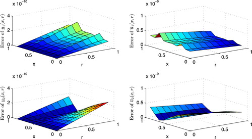by the presented method for N = 2, M = 3 and M = 6, respectively. Figs. 1 and 2 display absolute error functions obtained by the present method for N = 2, M = 3 and M = 6, respectively.

Fig. 1 Absolute error functions obtained by the present method for N = 2 and M = 3 of Example 2.

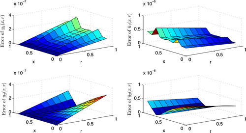
Fig. 2 Absolute error functions obtained by the present method for N = 2 and M = 6 of Example 2.

9 Conclusion

The fuzzy integral equations are important for studying and solving a large proportion of the problems in many topics in applied mathematics. In the present work the hybrid of Bernstein and block-pulse functions is used to solve linear fuzzy Fredholm integral equation systems. Also, we proved the convergence of this method. Illustrative numerical examples are included in order to test the accuracy and the convergence of the proposed method. In the above presented numerical examples we see that the proposed method well performs for system of linear fuzzy integral equations and the existence and convergence results (Theorems 2 and 3) are confirmed.

Acknowledgment

We are very grateful to an anonymous referee for the valuable comments and suggestions which have improved the manuscript.

Notes

Peer review under responsibility of Taibah University.