Mathematical model for cathodic protection in a steel-saline water system

Peer review under responsibility of Taibah University.

Abstract

The corrosion of steel tubes in sea water was controlled by cathodic protection. The impressed current technique was used. The rate of reaction was evaluated as a function of the temperature, pH and solution velocity. In this technique, the polarization method was used to determine the protection potential and current. The rate of zinc consumption, the protection potential, and the protection current are highly dependent on the variables of the study. The boundary element technique was suitable for modelling corrosion problems. The average percentage of error among the experimental and theoretical data was 1.27%.

Keywords:

• Corrosion
• Electrochemical method
• Metals
• Polarization
• Cathodic protection

1 Introduction

Among the various corrosion control methods available, cathodic protection is commonly adopted to control the corrosion of steel. The cathodic protection system is aimed to shift the potential of steel to the least probable range for corrosion [1]. The first attempts at cathodic protection modelling were made using finite difference approaches, but this technique is limited to two-dimensional and axisymmetric problems. Recently, the finite element method has been used successfully by some researchers [2]. Unlike other applications of the finite element method, the object of a cathodic protection system is not the structure itself but the environment close to the structure. Therefore, it is required to construct a finite element mesh of the medium between the members of the structure and to extend the mesh along the distance to establish a realistic boundary. The boundary element method requires only the discretization of the anode and cathode surfaces; therefore, the numerical problem may be reduced in size, which permits better resolution and a reduction in computer time compared to other methods, particularly for complex geometries [3]. Cathodic protection involves the application of a direct current (DC) from an anode through the electrolyte to the surface to be protected. This is often thought of as “overcoming” the corrosion currents that exist on the structure. Cathodic protection eliminates the potential differences between the anodes and cathodes on the corroding surface. A potential difference is then created between the cathodic protection anode and the structure such that the cathodic protection anode has a more negative potential than any point on the structure surface. Thus, the structure becomes the cathode of a new corrosion cell [4,5]. There are two methods for applying cathodic protection: sacrificial anode (galvanic) and impressed current. Each method depends on a number of economic and technical considerations. For every structure, there is a special cathodic protection system dependent on the environment of the structure [6]. Current distribution in a cathodic protection system is dependent on several factors, the most important of which are the driving potential, anode and cathode geometry, spacing between the anode and cathode and the conductivity of the aqueous environment, which is favourable for a good distribution of current [2,7]. Structures commonly protected are the exterior surfaces of pipelines, ships’ hulls, jetties, foundation piling, steel sheet-piling and offshore platforms. Cathodic protection is also used on the interior surfaces of water-storage tanks and water-circulating systems. However, because an external anode will seldom spread the protection over a distance of more than two or three pipe-diameters, the method is not suitable for the protection of small-bore pipe work. [8]. There have been many laboratory studies on the corrosion of mild steel in saline water, but the application of mathematical models has been limited. This is of particular interest in developing a better scientific understanding of corrosion processes. Therefore, the present work considered the two types of cathodic protection that were studied in our previous work [9,10] with the application of a mathematical model. This model was based on the boundary element method.

Symbols list
δ(|ζ − P|)	=	Dirac delta function
ζ − P	=	distance between the load point and the field point
ci	=	concentration of species i
$C_{{\text{O}}_2}$	=	concentration of oxygen
D	=	diffusivity of dissolved oxygen
Di	=	diffusion coefficient of species i
E	=	electrochemical potential
Ea	=	activation energy
Ep	=	protection potential
F	=	Faraday’s constant
I*	=	fundamental current density
Ij	=	component of the current density vector
J	=	mole flux of oxygen
k	=	rate constant of the reaction
kd	=	mass transfer coefficient
ko	=	constant
N	=	number of species
n	=	order of reaction
P	=	load point (source point)
R	=	universal gas constant
T	=	temperature
ui	=	mobility of species i
zi	=	charge of species i
ζ	=	field point or influence point (receiver point)
μ	=	sea water viscosity

2 Mathematical model derivation

Corrosion engineers are interested in knowing the current and potential on the metal surfaces after two metals are electrically connected. The main objective was to provide a uniform potential distribution on the metal surface for the minimum possible power input. If the cathodic protection technique is developed with a homogeneous region Ω surrounded by a boundary Γ and with electrical conductivity k, the equation which relates the current with the potential is [11]:(1) $I_j=-F\sum _{i=1}^N{z}_i{D}_i\frac{\partial c_i}{\partial x_j}-F^2\sum _{i=1}^N{z}_i^2{c}_i{u}_i\frac{\partial E}{\partial x_j}$(1)

Defining the conductivity of the electrolyte [12]:(2) $k=F^2\sum _{i=1}^N{z}_i^2{c}_i{u}_i$(2)

Eq. (1)(1) $I_j=-F\sum _{i=1}^N{z}_i{D}_i\frac{\partial c_i}{\partial x_j}-F^2\sum _{i=1}^N{z}_i^2{c}_i{u}_i\frac{\partial E}{\partial x_j}$(1) becomes:(3) $I_j=-F\sum _{i=1}^N{z}_i{D}_i\frac{\partial c_i}{\partial x_j}-k\frac{\partial E}{\partial x_j}$(3)

The first term of Eq. (3)(3) $I_j=-F\sum _{i=1}^N{z}_i{D}_i\frac{\partial c_i}{\partial x_j}-k\frac{\partial E}{\partial x_j}$(3) represents the portion of the current density sustained by the concentration gradient, which is generally neglected in large scale simulations. Eq. (3)(3) $I_j=-F\sum _{i=1}^N{z}_i{D}_i\frac{\partial c_i}{\partial x_j}-k\frac{\partial E}{\partial x_j}$(3) is reduced to:(4) $I_j=-k\frac{\partial E}{\partial x_j}$(4)

Conservation of charge requires that:(5) $\frac{\partial I_j}{\partial x_j}=\frac{\partial }{\partial x_j}\left(-k\frac{\partial E}{\partial x_j}\right)=0$(5)

The conductivity is assumed to be constant for sea water; thus, Eq. (5)(5) $\frac{\partial I_j}{\partial x_j}=\frac{\partial }{\partial x_j}\left(-k\frac{\partial E}{\partial x_j}\right)=0$(5) reduces to the Laplace equation for electrochemical potential [12–15]:(6) $k{\nabla }^{2}E=0$(6)

Or:(7) ${\nabla }^{2}E=0$(7) where ∇² = (∂²/∂²x) + (∂²/∂y²) + (∂²/∂z²).

The Laplace equation (Eq. (7)(7) ${\nabla }^{2}E=0$(7) ) is a boundary integral formulation for the electric field that provides direct relationship between the potential and current. The solution of this equation can be obtained by applying Green’s theorem, [16,17] and this solution is readily available [17,18]. To simplify the solution, many assumptions can be taken into account: the conductivity of sea water is assumed to be constant, each element has only one node and the shape function is constant and linear. The full details of these assumptions and the derivation of the boundary element model have been performed [8] and the following equation can be obtained:(8) $c(P)E(P)+\sum _{e=1}^{\epsilon }\left(\sum _{m=1}^M{E}_m^e{\int }_{{\Gamma }_e}I*(\zeta ,P){\varphi }_{m}d{\Gamma }_{\zeta }\right)=\sum _{e=1}^{\epsilon }\left(\sum _{m=1}^M{I}_m^e{\int }_{{\Gamma }_e}E*(\zeta ,P){\varphi }_{m}d{\Gamma }_{\zeta }\right)$(8) where the nodal values $E_m^e$ and $I_m^e$ are constants and can be brought outside the integrals. The principle of collocation means to locate the load point sequentially at all nodes of the discretization such that the domain variable at the load point E(P) coincides with the nodal value. Because linear and higher order polynomial shape functions lead to nodes that belong to more than one element, it is worthwhile to introduce a global node numbering (k = 1, …, K) that does not depend on the element. If the load point is located on the first global node, the first equation of the system reads:(9) $E_1\underset{{\hat{H}}_{11}}{\underbrace{\left({\int }_{\Gamma (1,e)}{\varphi }_{1}I*(\zeta ,P_1)d\Gamma +c_1\right)}}+E_2\underset{H_{12}}{\underbrace{{\int }_{\Gamma (2,e)}{\varphi }_{2}I*(\zeta ,P_1)d\Gamma }}+\cdots +E_K\underset{H_{1K}}{\underbrace{{\int }_{\Gamma (K,e)}{\varphi }_{K}I*(\zeta ,P_1)d\Gamma }}=I_1\underset{G_{11}}{\underbrace{{\int }_{\Gamma (1,e)}{\varphi }_{1}E*(\zeta ,P_1)d\Gamma }}+I_2\underset{G_{12}}{\underbrace{{\int }_{\Gamma (2,e)}{\varphi }_{2}E*(\zeta ,P_1)d\Gamma }}+\cdots +I_K\underset{G_{1K}}{\underbrace{{\int }_{\Gamma (K,e)}{\varphi }_{K}E*(\zeta ,P_1)d\Gamma }}$(9)

The notation ∫_Γ(k,e)dΓ means the sum of integrals contributed from these elements that contain the global node, where Φ_k is the corresponding shape function. In matrix form, Eq. (9)(9) $E_1\underset{{\hat{H}}_{11}}{\underbrace{\left({\int }_{\Gamma (1,e)}{\varphi }_{1}I*(\zeta ,P_1)d\Gamma +c_1\right)}}+E_2\underset{H_{12}}{\underbrace{{\int }_{\Gamma (2,e)}{\varphi }_{2}I*(\zeta ,P_1)d\Gamma }}+\cdots +E_K\underset{H_{1K}}{\underbrace{{\int }_{\Gamma (K,e)}{\varphi }_{K}I*(\zeta ,P_1)d\Gamma }}=I_1\underset{G_{11}}{\underbrace{{\int }_{\Gamma (1,e)}{\varphi }_{1}E*(\zeta ,P_1)d\Gamma }}+I_2\underset{G_{12}}{\underbrace{{\int }_{\Gamma (2,e)}{\varphi }_{2}E*(\zeta ,P_1)d\Gamma }}+\cdots +I_K\underset{G_{1K}}{\underbrace{{\int }_{\Gamma (K,e)}{\varphi }_{K}E*(\zeta ,P_1)d\Gamma }}$(9) is:(10) $\left[\begin{array}{cccc}\hfill {\hat{H}}_{11}\hfill & \hfill H_{12}\hfill & \hfill \mathrm{....}\hfill & \hfill H_{1K}\hfill \end{array}\right]\left[\begin{array}{c}\hfill E_1\hfill \\ \hfill E_2\hfill \\ \hfill :\hfill \\ \hfill E_K\hfill \end{array}\right]=\left[\begin{array}{cccc}\hfill G_{11}\hfill & \hfill G_{12}\hfill & \hfill \mathrm{....}\hfill & \hfill G_{1K}\hfill \end{array}\right]\left[\begin{array}{c}\hfill I_1\hfill \\ \hfill I_2\hfill \\ \hfill :\hfill \\ \hfill I_K\hfill \end{array}\right]$(10) where (^∧) denotes the element that contains the boundary term c(ζ). By collocation of the load point with nodes 2 to K, the additional equation of the system, Eq. (11)(11) $\left[\begin{array}{cccc}\hfill H_{11}\hfill & \hfill H_{12}\hfill & \hfill \mathrm{....}\hfill & \hfill H_{1K}\hfill \\ \hfill H_{21}\hfill & \hfill {\hat{H}}_{22}\hfill & \hfill \mathrm{....}\hfill & \hfill H_{2K}\hfill \\ \hfill :\hfill & \hfill \hfill & \hfill \hfill & \hfill :\hfill \\ \hfill H_{K1}\hfill & \hfill H_{K2}\hfill & \hfill \mathrm{....}\hfill & \hfill {\hat{H}}_{KK}\hfill \end{array}\right]\left[\begin{array}{c}\hfill E_1\hfill \\ \hfill E_2\hfill \\ \hfill :\hfill \\ \hfill E_K\hfill \end{array}\right]=\left[\begin{array}{cccc}\hfill G_{11}\hfill & \hfill G_{12}\hfill & \hfill \mathrm{....}\hfill & \hfill G_{1K}\hfill \\ \hfill G_{21}\hfill & \hfill G_{22}\hfill & \hfill \mathrm{....}\hfill & \hfill G_{2K}\hfill \\ \hfill :\hfill & \hfill \hfill & \hfill \hfill & \hfill :\hfill \\ \hfill G_{K1}\hfill & \hfill G_{K2}\hfill & \hfill \mathrm{....}\hfill & \hfill G_{KK}\hfill \end{array}\right]\left[\begin{array}{c}\hfill I_1\hfill \\ \hfill I_2\hfill \\ \hfill \begin{array}{l}:\\ \end{array}\hfill \\ \hfill I_K\hfill \end{array}\right]$(11) is obtained:(11) $\left[\begin{array}{cccc}\hfill H_{11}\hfill & \hfill H_{12}\hfill & \hfill \mathrm{....}\hfill & \hfill H_{1K}\hfill \\ \hfill H_{21}\hfill & \hfill {\hat{H}}_{22}\hfill & \hfill \mathrm{....}\hfill & \hfill H_{2K}\hfill \\ \hfill :\hfill & \hfill \hfill & \hfill \hfill & \hfill :\hfill \\ \hfill H_{K1}\hfill & \hfill H_{K2}\hfill & \hfill \mathrm{....}\hfill & \hfill {\hat{H}}_{KK}\hfill \end{array}\right]\left[\begin{array}{c}\hfill E_1\hfill \\ \hfill E_2\hfill \\ \hfill :\hfill \\ \hfill E_K\hfill \end{array}\right]=\left[\begin{array}{cccc}\hfill G_{11}\hfill & \hfill G_{12}\hfill & \hfill \mathrm{....}\hfill & \hfill G_{1K}\hfill \\ \hfill G_{21}\hfill & \hfill G_{22}\hfill & \hfill \mathrm{....}\hfill & \hfill G_{2K}\hfill \\ \hfill :\hfill & \hfill \hfill & \hfill \hfill & \hfill :\hfill \\ \hfill G_{K1}\hfill & \hfill G_{K2}\hfill & \hfill \mathrm{....}\hfill & \hfill G_{KK}\hfill \end{array}\right]\left[\begin{array}{c}\hfill I_1\hfill \\ \hfill I_2\hfill \\ \hfill \begin{array}{l}:\\ \end{array}\hfill \\ \hfill I_K\hfill \end{array}\right]$(11)

And read in matrix notation:(12) $\text{HE}=\text{GI}$(12)

The diagonal elements of the matrices H and G contain singular integrals because the distance |ζ − P| vanishes at the nodes. All other matrix elements contain regular integrals.

3 Experimental data

In our previous work, the application of the cathodic protection technique was studied [9,10]. Impressed current techniques were applied successfully. In this technique, the experimental work was conducted to determine the potential and current density required in cathodic protection using polarization techniques for various conditions of temperature (0–45 °C), rotating velocity (0–400 rpm) and pH (2–12) [9,10]. The results of the above works were used as the feed data of the mathematical model.

4 Results and discussion of the fundamental solution (E*, I*), example of the numerical solution and comparison with the experimental values

For two dimensions and for simplicity, the load point is shifted to the origin, and constant elements with only one node located in the middle are chosen (i.e., M = 1, Φ = 1 and c(P) = 1/2). Laplace’s equation of potential distribution is considered in the following example of a 2D rectangular domain with an aspect ratio 1:2, as depicted in Fig. 1. If Eq. (8)(8) $c(P)E(P)+\sum _{e=1}^{\epsilon }\left(\sum _{m=1}^M{E}_m^e{\int }_{{\Gamma }_e}I*(\zeta ,P){\varphi }_{m}d{\Gamma }_{\zeta }\right)=\sum _{e=1}^{\epsilon }\left(\sum _{m=1}^M{I}_m^e{\int }_{{\Gamma }_e}E*(\zeta ,P){\varphi }_{m}d{\Gamma }_{\zeta }\right)$(8) is written for the load point P, the following equation can be obtained:(13) $\begin{array}{l}\frac{1}{2}E(P_l)+{\displaystyle \sum }_{e=1}^{\epsilon }\left(\frac{(\zeta -P)}{2\pi \text{|}\zeta -P{\text{|}}^2}d\Gamma \right)E_e\\ ={\displaystyle \sum }_{e=1}^{\epsilon }\left(-\frac{1}{2\pi }\ln \left|\zeta -P\right|d\Gamma \right)I_e\end{array}$(13) l is the iteration of the load point, P. Four equations for four unknown boundary values are obtained if l takes the values 1–4 and P_l is located at the four nodes sequentially. The elements of the matrices are the integrals in Eq. (13)(13) $\begin{array}{l}\frac{1}{2}E(P_l)+{\displaystyle \sum }_{e=1}^{\epsilon }\left(\frac{(\zeta -P)}{2\pi \text{|}\zeta -P{\text{|}}^2}d\Gamma \right)E_e\\ ={\displaystyle \sum }_{e=1}^{\epsilon }\left(-\frac{1}{2\pi }\ln \left|\zeta -P\right|d\Gamma \right)I_e\end{array}$(13) for different values of l and e. In matrix form:(14) $\frac{1}{2}\left[\begin{array}{c}\hfill E_1\hfill \\ \hfill E_2\hfill \\ \hfill E_3\hfill \\ \hfill E_4\hfill \end{array}\right]+\text{H}\left[\begin{array}{c}\hfill E_1\hfill \\ \hfill E_2\hfill \\ \hfill E_3\hfill \\ \hfill E_4\hfill \end{array}\right]=\text{G}\left[\begin{array}{c}\hfill I_1\hfill \\ \hfill I_2\hfill \\ \hfill I_3\hfill \\ \hfill I_4\hfill \end{array}\right]$(14)

Fig. 1 Calculation matrix elements H₁₂ and G₁₂ for the potential distribution in a rectangular domain. Note: the common notation ζ for field point (marked by $\overrightarrow{n}$) and load point P (marked by $\overrightarrow{P}$).

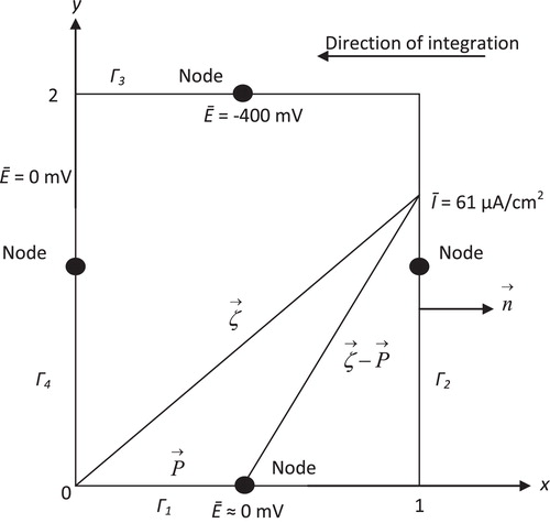
The boundary conditions were taken as a temperature of 22.5 °C, rotating velocity of 0 rpm and pH 7. With these boundary conditions, at node 1 (element 1), ${\overline{E}}_1$ is the IR voltage between the cathode and anode ≈ 0, at node 2 (element 2) the current density of the cathode i_p = 61 μA/cm², at node 3 (element 3), which is the wire connection between the anode and cathode, the potential is −400 mV and at anode 4 (element 4), the potential of anode is equal to 0. Furthermore:(15) $\left.\begin{array}{l}{\text{H}}_{14}={\text{H}}_{34}={\text{H}}_{32}={\text{H}}_{12}\\ {\text{G}}_{14}={\text{G}}_{34}={\text{G}}_{32}={\text{G}}_{12}\end{array}\right\}$(15)

Spatial isotropy leads to:(16) $\left.\begin{array}{l}{\text{H}}_{21}={\text{H}}_{41}={\text{H}}_{43}={\text{H}}_{23}\\ {\text{G}}_{21}={\text{G}}_{41}={\text{G}}_{43}={\text{G}}_{23}\end{array}\right\}$(16)

And by virtue of symmetry:(17) ${\text{H}}_{31}={\text{H}}_{13}\text{and}{\text{G}}_{31}={\text{G}}_{13}$(17) (18) ${\text{H}}_{42}={\text{H}}_{24}\text{and}{\text{G}}_{42}={\text{G}}_{24}$(18)

The main diagonal of matrix H vanishes:(19) ${\text{H}}_{11}={\text{H}}_{22}={\text{H}}_{33}={\text{H}}_{44}=0$(19)

Because of symmetry:(20) ${\text{G}}_{33}={\text{G}}_{11}$(20) (21) ${\text{G}}_{44}={\text{G}}_{22}$(21)

Rewriting Eq. (14)(14) $\frac{1}{2}\left[\begin{array}{c}\hfill E_1\hfill \\ \hfill E_2\hfill \\ \hfill E_3\hfill \\ \hfill E_4\hfill \end{array}\right]+\text{H}\left[\begin{array}{c}\hfill E_1\hfill \\ \hfill E_2\hfill \\ \hfill E_3\hfill \\ \hfill E_4\hfill \end{array}\right]=\text{G}\left[\begin{array}{c}\hfill I_1\hfill \\ \hfill I_2\hfill \\ \hfill I_3\hfill \\ \hfill I_4\hfill \end{array}\right]$(14) in index notation and summation of the E terms leads to:(22) $\left(\frac{1}{2}+{\text{H}}_{le}\right){\text{E}}_e={\text{G}}_{le}{\text{I}}_e$(22)

Plugging the matrix elements and the known boundary data rearrangement leads to:$\left[\begin{array}{cccc}\hfill 0.5000\hfill & \hfill -0.1621\hfill & \hfill 0.0780\hfill & \hfill 0.1621\hfill \\ \hfill 0.9653\hfill & \hfill -0.5000\hfill & \hfill 0.9653\hfill & \hfill 0.42\hfill \\ \hfill 0.0780\hfill & \hfill -0.1621\hfill & \hfill 0.5000\hfill & \hfill 0.1621\hfill \\ \hfill 0.9653\hfill & \hfill -0.42\hfill & \hfill 0.9653\hfill & \hfill 0.5000\hfill \end{array}\right]\left[\begin{array}{c}\hfill {\overline{E}}_1=0\hfill \\ \hfill {\overline{E}}_2\hfill \\ \hfill {\overline{E}}_3=-400\hfill \\ \hfill {\overline{E}}_4=0\hfill \end{array}\right]=\left[\begin{array}{cccc}\hfill 0.2695\hfill & \hfill -0.0175\hfill & \hfill -0.1119\hfill & \hfill -0.0175\hfill \\ \hfill -0.0210\hfill & \hfill 0.3183\hfill & \hfill -0.210\hfill & \hfill -0.0420\hfill \\ \hfill -0.1119\hfill & \hfill -0.0175\hfill & \hfill -0.2695\hfill & \hfill -0.0175\hfill \\ \hfill -0.0210\hfill & \hfill -0.0420\hfill & \hfill -0.0210\hfill & \hfill 0.3183\hfill \end{array}\right]\left[\begin{array}{c}\hfill I_1\hfill \\ \hfill I_2=61\hfill \\ \hfill I_3\hfill \\ \hfill I_4\hfill \end{array}\right]$

After rewriting the equations with all unknown boundary data appearing on the left side.$\left[\begin{array}{cccc}\hfill -0.2695\hfill & \hfill -0.1621\hfill & \hfill 0.1119\hfill & \hfill 0.0175\hfill \\ \hfill 0.0210\hfill & \hfill -0.5000\hfill & \hfill 0.0210\hfill & \hfill 0.0420\hfill \\ \hfill 0.1119\hfill & \hfill -0.1621\hfill & \hfill -0.2695\hfill & \hfill 0.0175\hfill \\ \hfill 0.0210\hfill & \hfill -0.4200\hfill & \hfill 0.0210\hfill & \hfill -0.3183\hfill \end{array}\right]\left[\begin{array}{c}\hfill I_1\hfill \\ \hfill E_2\hfill \\ \hfill I_3\hfill \\ \hfill I_4\hfill \end{array}\right]=\left[\begin{array}{cccc}\hfill 0.5000\hfill & \hfill -0.0175\hfill & \hfill -0.0780\hfill & \hfill -0.1621\hfill \\ \hfill -0.9653\hfill & \hfill 0.3183\hfill & \hfill -0.9653\hfill & \hfill -0.4200\hfill \\ \hfill -0.0780\hfill & \hfill -0.0175\hfill & \hfill -0.5000\hfill & \hfill -0.1621\hfill \\ \hfill -0.9653\hfill & \hfill -0.4200\hfill & \hfill -0.9653\hfill & \hfill -0.5000\hfill \end{array}\right]\left[\begin{array}{c}\hfill 0\hfill \\ \hfill 61\hfill \\ \hfill -400\hfill \\ \hfill 0\hfill \end{array}\right]$

Solving the equations leads to:$\left[\begin{array}{c}\hfill I_1\hfill \\ \hfill E_2\hfill \\ \hfill I_3\hfill \\ \hfill I_4\hfill \end{array}\right]=\left[\begin{array}{c}\hfill 265\mu {\text{A/cm}}^2\hfill \\ \hfill -816\text{mV}\hfill \\ \hfill -265\mu {\text{A/cm}}^2\hfill \\ \hfill -58.3\mu {\text{A/cm}}^2\hfill \end{array}\right]$

Experimentally, E₂ = −805 mV; thus, the error is as 1.37%. For protection, the summation of currents must be equal to zero [19]. Algebraic addition gives 61 + 265 − 58.3 − 265 = 2.7 μA/cm² (too small). The results of the mathematical models are in good agreement with the experimental results. Table 1 shows the values of the experimental protection potential compared with the protection potential obtained from the boundary element model. Good agreement is obtained at all boundary conditions.

Table 1 Results of the protection potentials with different conditions.

Run no.	X1	X2	X3	Ep, (Exp.) mV	Ep, (Theo.) mV	Absolute % error
1	9.5	85	4.11	−820	−825	0.61
2	9.5	85	9.89	−800	−820	2.51
3	9.5	315	4.11	−825	−833	0.97
4	9.5	315	9.89	−800	−811	1.37
5	35.5	85	4.11	−825	−834	1.09
6	35.5	85	9.89	−800	−814	1.75
7	35.5	315	4.11	−830	−840	1.21
8	35.5	315	9.89	−805	−817	1.49
9	0.0	200	7.00	−805	−809	0.49
10	45.0	200	7.00	−810	−818	0.98
11	22.5	0	7.00	−805	−816	1.36
12	22.5	400	7.00	−810	−819	1.11
13	22.5	200	2.00	−850	−865	1.76
14	22.5	200	12.00	−790	−799	1.14
15–18	22.5	200	7.00	−805	−818	1.61

X₁ is the temperature range between 0 and 45 °C, X₂ is the rotating velocity range between 0 and 400 rpm, and X₃ is the pH range between 2 and 12 [9,10].

Conclusions

The boundary element technique was suitable for modelling corrosion problems when the surface has to be defined. The values of the potential and current density can be computed with high accuracy. Good agreement between experimental and theoretical values was obtained.

Acknowledgement

This work was supported by Baghdad University, Chemical Engineering Department, which is gratefully acknowledged.

Notes

Peer review under responsibility of Taibah University.