Polarized-radiation transfer in stochastic finite planar atmospheric media

Peer review under responsibility of Taibah University

Abstract

In this work, we investigate the polarized-radiation transfer problem in a planar stochastic atmospheric medium. A solution is presented for an arbitrary extinction function, which was assumed to be continuous in position and to exhibit fluctuations about the Gaussian distributed mean. The joint probability distribution function of the integral transform of these Gaussian random functions was used to calculate the ensemble-averaged quantities, such as the reflectivity and transmissivity, for an arbitrary correlation function. A modified Gaussian probability distribution function was used to average the solution to exclude probable negative values of the optical space variable. The deterministic solutions for the total intensity and the difference function, which were used to describe the polarized radiation, were obtained using the Pomraning–Eddington technique. The numerical results were presented for the Gaussian and modified Gaussian probability density functions for different degrees of polarization.

Keywords:

• Polarized-radiation transfer
• Stochastic atmospheric medium
• Gaussian statistics

1 Introduction

It is well known that the scattering by particles (aerosols, cloud drops, crystals, molecules and atoms) induces polarization in incident unpolarized radiation beams or modifies the initial polarization. Hence, an exact treatment of light propagation in a medium composed of such scattering particles must include the state of radiation polarization both before and after scattering. Therefore, the study of polarized-radiation transfer in stochastic media is of great interest with regard to planetary atmospheres. The first formulation of such a problem allowing polarization was developed by Chandrasekhar [1] to describe the spatial variation of the four Stokes parameters: I, K, U, and V.

There has been an increasing interest in the use of polarization in imaging through cluttered media (stochastic media). Optical imaging through clouds and fog, and microwave detection in clutter can benefit from the additional information provided by the polarization characteristics [2]. Polarization pulse propagation in random media has also received attention, with most of these studies using Monte Carlo calculations [3].

Radiative transfer computations of the Earth's atmospheres continue to become more important as the emphasis on remote sensing shifts towards understanding the microphysical properties of clouds. In addition to a better understanding of the nonlinear relationships between rainfall rates and satellite-observed radiances [4], a large interest has developed in sub-mm ice clouds studies [5,6]. To achieve these goals, significant attention is being given to the polarization effects from emission/scattering due to particles and surfaces. Simulations of polarized-radiation transfer can yield results on this subject [7–9].

The study of radiative transfer with polarization in a finite plane-parallel stochastic atmospheric medium (such as clouds and fog) is presented in this paper. It is reasonable to characterize the stochastic atmospheric medium in a statistical sense. This requires specifying the probability distribution of fluctuating properties via spatial and temporal correlations, etc. A stochastic transport class of problems arises when the environmental properties of the background medium are random functions of position and time that are in scales on the order of, or longer than, several mean free paths.

Throughout this work, the atmospheric medium is considered to be a continuously stochastic background. The extinction function of the medium is assumed to be a continuous random function of position, with fluctuations about the mean taken as being Gaussian distributed. The joint probability distribution function of these Gaussian random variables is used to calculate the ensemble-averaged quantities, such as the average reflectivity and transmissivity over the medium fluctuations, for an arbitrary correlation function. The Pomraning–Eddington approximation is employed to yield deterministic solutions for the total intensity and the difference function of the polarized radiation [8,9]. Then, the solution is averaged using a Gaussian joint probability distribution function [10,11]. However, a weakness of the Gaussian model is that the random variables that are physically constrained to be positive can in fact, from mathematical point of view, take on negative values, albeit with an exponentially decreasing probability. This can potentially be cause for concern when ensemble averages are considered, especially when the fluctuation amplitude is large. Hence, a modified Gaussian probability density function [11] is used to overcome this defect. Numerical results are presented for both the average reflectivity 〈R〉 and transmissivity 〈T〉 for different degrees of polarization and values of the scattering albedo.

2 Basic equations

Considering the Rayleigh scattering phase function with polarization, the scalar radiative transfer equation(1) $\left(\mu \frac{\partial }{\partial x}+1\right)I\left(x,\mu \right)=\frac{\omega }{2}{\int }_{-1}^{1}P\left(\mu ,{\mu }^{\prime }\right)I\left(x,{\mu }^{\prime }\right)d{\mu }^{\prime }$(1) should be replaced by the two coupled equations describing the transfer of linearly polarized radiation [1,12] as(2) $\left(\mu \frac{\partial }{\partial x}+1\right)I(x,\mu )=\frac{\omega }{2}{\int }_{-1}^{1}d{\mu }^{\prime }\left\{\left[1+\frac{1}{2}{P}_2(\mu )P_2\left({\mu }^{\prime }\right)\right]I\left(x,{\mu }^{\prime }\right)-\frac{1}{2}{P}_2(\mu )\left[1-P_2\left({\mu }^{\prime }\right)\right]K\left(x,{\mu }^{\prime }\right)\right\}$(2) and(3) $\left(\mu \frac{\partial }{\partial x}+1\right)K(x,\mu )=\frac{\omega }{4}[1-P_2(\mu )]{\int }_{-1}^{1}d{\mu }^{\prime }\left\{\left[1-P_2\left({\mu }^{\prime }\right)\right]K\left(x,{\mu }^{\prime }\right)-P_2\left({\mu }^{\prime }\right)I\left(x,{\mu }^{\prime }\right)\right\},0\le x\le L,-1\le \mu \le 1$(3) where I is the total intensity, I = I_l + I_r, and K is the difference function, K = I_l − I_r, which are the main parameters used to define the Stokes parameters, whereas the other two parameters vanish for linearly polarized radiation $\left(U=V=0\right)$. The variable P₂(μ) represents a second-order Legendre polynomial P₂(μ) = 0.5(3μ² − 1).

The boundary conditions for the finite medium are assumed to be(4) $\begin{array}{l}I(0,\mu )=\Gamma (\mu ),K(0,\mu )={\alpha }^{*}(\mu )\Gamma (\mu )\\ I(L,-\mu )=0,K(L,-\mu )=0\end{array}$(4) where Γ(μ) is the angle-dependent externally incident flux. The quantity α*(μ) describes the degree of polarization at a given angle. Natural (unpolarized) radiation corresponds to α* = 0 and α* = ±1 represent the two polarization extremes.

Using the Pomraning–Eddington approximation [8] for both the total intensity and the difference function yields(5) $\begin{array}{c}\hfill I\left(x,\mu \right)={\epsilon }_1\left(x,\mu \right)E_1\left(x\right)+O_1\left(x,\mu \right)F_1\left(x\right)\hfill \\ \hfill K\left(x,\mu \right)={\epsilon }_2\left(x,\mu \right)E_2\left(x\right)+O_2\left(x,\mu \right)F_2\left(x\right)\hfill \end{array}$(5) where ${\epsilon }_i\left(x,\mu \right)$ and $O_i\left(x,\mu \right)$ $\left\{i=\mathrm{1,2}\right\}$ are even and odd functions in μ, which are assumed to be slowly varying functions in x and are normalized as(6) ${\int }_{-1}^1{\epsilon }_i\left(x,\mu \right)d\mu ={\int }_{-1}^1\mu O_i\left(x,\mu \right)d\mu =1$(6)

The radiant energies E_i(x) and the net fluxes F_i(x) are defined as(7) $\begin{array}{l}{E}_1(x)={\int }_{-1}^{1}I(x,\mu )d\mu ,E_2(x)={\int }_{-1}^{1}K(x,\mu )d\mu \\ F_1(x)={\int }_{-1}^1\mu I(x,\mu )d\mu ,F_2(x)={\int }_{-1}^1\mu K(x,\mu )d\mu \end{array}$(7)

Following the procedure described in [8,9], we arrive at the solution of Eq. (2)(2) $\left(\mu \frac{\partial }{\partial x}+1\right)I(x,\mu )=\frac{\omega }{2}{\int }_{-1}^{1}d{\mu }^{\prime }\left\{\left[1+\frac{1}{2}{P}_2(\mu )P_2\left({\mu }^{\prime }\right)\right]I\left(x,{\mu }^{\prime }\right)-\frac{1}{2}{P}_2(\mu )\left[1-P_2\left({\mu }^{\prime }\right)\right]K\left(x,{\mu }^{\prime }\right)\right\}$(2) and (3)(3) $\left(\mu \frac{\partial }{\partial x}+1\right)K(x,\mu )=\frac{\omega }{4}[1-P_2(\mu )]{\int }_{-1}^{1}d{\mu }^{\prime }\left\{\left[1-P_2\left({\mu }^{\prime }\right)\right]K\left(x,{\mu }^{\prime }\right)-P_2\left({\mu }^{\prime }\right)I\left(x,{\mu }^{\prime }\right)\right\},0\le x\le L,-1\le \mu \le 1$(3) :(8) $I\left(x,\mu \right)=A_1{H}_{+}\left(\mu \right)e^{k_{1}x}+B_1{H}_{-}\left(\mu \right)e^{-k_{1}x}$(8) and(9) $K(x,\mu )=A_2{G}_{+}(\mu )e^{k_{2}x}+B_2{G}_{-}(\mu )e^{-k_{2}x}+\frac{\lambda k_2^2}{{\alpha }_2}\frac{{\epsilon }_2(x,\mu )}{k_2^2-k_1^2}[A_1(1-k_1\mu )e^{k_{1}x}+B_1(1+k_1\mu )e^{-k_{1}x}]$(9) where(10) $H_{\pm }\left(\mu \right)=\frac{\omega }{2}\frac{1+{\phi }_1{P}_2\left(\mu \right)}{1\pm k_1\mu },\text{and}{G}_{\pm }(\mu )=\frac{\omega }{4}\frac{{\phi }_2\left(1\mp k_2\mu \right)\left[1-P_2\left(\mu \right)\right]}{1-k_2^{*2}{\mu }^2}$(10) with(11) ${\phi }_1=\frac{1}{4}(3{\delta }_1-1)-\frac{3{\alpha }^{*}}{4}(1-{\delta }_2),{\phi }_2=\frac{3}{2}*(1-{\delta }_2)-\frac{1}{2{\alpha }^{*}}(3{\delta }_1-1)\text{,}$(11) (12) $k_1=\sqrt{\frac{{\alpha }_1}{{\delta }_1}},k_2=\sqrt{\frac{{\alpha }_2}{{\delta }_2}},k_2^{*}=\sqrt{\frac{{\alpha }_2-\lambda /{\alpha }^{*}}{{\delta }_2}},{\alpha }_1=1-\omega ,{\alpha }_2=1-\frac{3\omega }{4}(1-{\delta }_2),\lambda =\frac{\omega }{4}(1-3{\delta }_2)$(12)

We define(13) ${\delta }_i={\int }_{-1}^1{\mu }^2{\epsilon }_i(x,\mu )d\mu ,i=\mathrm{1,2}$(13) where the even functions ${\epsilon }_i\left(x,\mu \right)$ are obtained from [8,9]. To determine the values of the constants A_i and B_i, a weighted function $W\left(\mu \right)$ is introduced to force boundary condition (4) to be fulfilled as(14) $\begin{array}{c}\hfill {\int }_0^{1}W(\mu )I(0,\mu )d\mu =I_0,{\int }_0^{1}W(\mu )K\left(0,\mu \right)d\mu ={\alpha }^{*}{I}_0\hfill \\ \hfill {\int }_0^{1}W(\mu )I(L,-\mu )d\mu =0,{\int }_0^{1}W(\mu )K\left(L,-\mu \right)d\mu =0\hfill \end{array}$(14) which can be solved simultaneously to yield the constants A_i and B_i, with $I_0={\int }_0^{1}W(\mu )\Gamma (\mu )d\mu$.

3 Statistical analysis

The starting point for the analysis is the scalar radiative transfer equation in a planar medium, which is given by [1](15) $\left[\mu \frac{\partial }{\partial z}+\sigma (z)\right]\Psi (z,\mu )=\frac{{\sigma }_s(z)}{2}{\int }_{-1}^{1}P\left(\mu ,{\mu }^{\prime }\right)\Psi \left(z,{\mu }^{\prime }\right)d{\mu }^{\prime },0\le z\le Z_0$(15) where Ψ(z, μ) is the radiation intensity, with z and Z0 denoting the geometric depth space variable and geometric thickness, respectively. The variable μ is the angular variable corresponding to the directional cosine of the propagating radiation. The quantity σ(z) is the extinction function and σ_s(z) is the scattering cross-section. The variable P(μ, μ′) represents the scattering phase function.

It is convenient to write Eq. (15)(15) $\left[\mu \frac{\partial }{\partial z}+\sigma (z)\right]\Psi (z,\mu )=\frac{{\sigma }_s(z)}{2}{\int }_{-1}^{1}P\left(\mu ,{\mu }^{\prime }\right)\Psi \left(z,{\mu }^{\prime }\right)d{\mu }^{\prime },0\le z\le Z_0$(15) in terms of the optical depth space variable as $x(z)={\int }_0^z\sigma (z)dz$, with the optical thickness $L(Z_0)={\int }_0^{Z_0}\sigma (z)dz$. Then, Eq. (15)(15) $\left[\mu \frac{\partial }{\partial z}+\sigma (z)\right]\Psi (z,\mu )=\frac{{\sigma }_s(z)}{2}{\int }_{-1}^{1}P\left(\mu ,{\mu }^{\prime }\right)\Psi \left(z,{\mu }^{\prime }\right)d{\mu }^{\prime },0\le z\le Z_0$(15) takes the same form as in Eq. (1)(1) $\left(\mu \frac{\partial }{\partial x}+1\right)I\left(x,\mu \right)=\frac{\omega }{2}{\int }_{-1}^{1}P\left(\mu ,{\mu }^{\prime }\right)I\left(x,{\mu }^{\prime }\right)d{\mu }^{\prime }$(1) , where $\Psi \left(z,\mu \right)\equiv I\left(x,\mu \right)$ and the single scattering albedo of the medium is ω = σ_s/σ.

The aim of modelling stochastic media is to find a radiative transfer equation with averaged or effective parameters that allows the calculation of the radiation transfer through the stochastic medium knowledge of the detailed structure of the medium.

3.1 The stochasticity of the extinction function σ(z)

In the usual (nonstochastic) application of the transport equation, as shown in Eq. (15)(15) $\left[\mu \frac{\partial }{\partial z}+\sigma (z)\right]\Psi (z,\mu )=\frac{{\sigma }_s(z)}{2}{\int }_{-1}^{1}P\left(\mu ,{\mu }^{\prime }\right)\Psi \left(z,{\mu }^{\prime }\right)d{\mu }^{\prime },0\le z\le Z_0$(15) , the extinction function, σ(z) and the scattering cross section, σs(z) are known (deterministic) and prescribed functions. In the stochastic setting, σ(z) and σs(z) are only known in some probabilistic sense. That is, at each space point z, there is some probability that each of these two quantities will assume certain values. Accordingly, we consider σ(z) and σs(z) to be random functions, with Ψ(z, μ) also being random. Upon transforming Eq. (1)(1) $\left(\mu \frac{\partial }{\partial x}+1\right)I\left(x,\mu \right)=\frac{\omega }{2}{\int }_{-1}^{1}P\left(\mu ,{\mu }^{\prime }\right)I\left(x,{\mu }^{\prime }\right)d{\mu }^{\prime }$(1) from a geometrical space to an optical space, as defined in Eq. (1)(1) $\left(\mu \frac{\partial }{\partial x}+1\right)I\left(x,\mu \right)=\frac{\omega }{2}{\int }_{-1}^{1}P\left(\mu ,{\mu }^{\prime }\right)I\left(x,{\mu }^{\prime }\right)d{\mu }^{\prime }$(1) , the stochastic nature of the problem is absorbed in the optical variable x. It is also assumed here that the cross section is a random function of the position, such that the single scattering albedo ω = σ_s/σ is non-random.

Assuming that the mean value of σ(z) includes fluctuations about this mean, ξ(z) is described by a Gaussian distribution, and we may express σ(z) = 〈 σ(z) 〉 + ξ(z), where ξ(z) describes the deviation of the extinction function from the mean. From a probabilistic point of view, the Gaussian random function, σ(z), is defined completely if its mean, $\overline{\sigma }=〈\sigma (z)〉$, and its autocorrelation function, W_σ(z₁, z₂), are defined. The autocorrelation function can be defined as:(16) $W_{\sigma }(z_1,z_2)=〈\xi (z_1)\xi (z_2)〉=〈[{\sigma }_1(z_1)-\overline{\sigma }][{\sigma }_2(z_2)-\overline{\sigma }]〉\text{,}$(16) where z1 and z2 are arbitrary positions. For homogeneous statistics, W_σ(z₁, z₂) depends on $\left|z_1-z_2\right|$, as

$W_{\sigma }(z_1,z_2)=W_{\sigma }\left(\left|z_1-z_2\right|\right)={\eta }_{\sigma }^{2}B\left(\left|z_1-z_2\right|\right)$ where the variance ${\eta }_{\sigma }^2=〈{[\sigma (z)-\overline{\sigma }]}^2〉>0$

We assume that the function W_σ(z₁, z₂) is positive for real values of z. Moreover, $W_{\sigma }(0)={\eta }_{\sigma }^2$ and W_σ(z) → 0 if $\left|z\right|\to \infty$. The shape function, B, describes the range over which the fluctuation parameters are correlated. It is typically characterized by the correlation length ℓ such that B ≈ 0 for $\left|z_1-z_2\right|>>\ell$ and $B\left(0\right)=1$. The form of B depends on the specific application, but in many cases, it is modelled by simple exponentials. However, the shape function is a deterministic function and must be provided in advance. Important and commonly employed models include the exponential functions [10,11](17) $B\left(\left|z\right|\right)=\exp \left(-\frac{\left|z\right|}{\ell }\right),orB\left(\left|z\right|\right)=\exp \left(-\frac{z^2}{{\ell }^2}\right)$(17)

If σ₁ and σ₂ are two Gaussian random functions, then σ₁ + σ₂ is also a Gaussian random function. Generalizing this statement, we may say that if $\sigma \left(z\right)$ is a Gaussian random function, then the optical depth space variable x is also Gaussian. The mean value of x is $\overline{x}=〈x〉={\int }_0^{z}d{z}^{\prime }〈\sigma \left(z^{\prime }\right)〉=\overline{\sigma }z$ and the mean value of the medium thickness is $\overline{L}=〈L〉={\int }_0^{Z_0}d{z}^{\prime }〈\sigma \left(z^{\prime }\right)〉=\overline{\sigma }{Z}_0$.

The variance η² of x depends on the form of the function $W\left(\left|z\right|\right)$ and can be written as(18) ${\eta }^2=〈{(x-\overline{x})}^2〉={\int }_0^{z}d{z}_1{\int }_0^{z}d{z}_2〈[\sigma (z_1)-\overline{\sigma }][\sigma (z_2)-\overline{\sigma }]〉={\int }_0^{z}d{z}_1{\int }_0^{z}d{z}_2{W}_{\sigma }\left(\left|z_1-z_2\right|\right)$(18)

We refrain from calculating the parameter η and we require that $0<{\eta }_{\sigma }<<\overline{x}$.

However, the randomness of the function σ(z) is defined by three parameters: $\overline{\sigma },{\eta }_{\sigma }$ and the correlation length ℓ. If η_σ → 0⁺, our stochastic problem becomes deterministic. The mean value $\overline{x}$ is a dimensionless quantity that is proportional to the factual length z. It is suitable to introduce a positive dimensionless parameter(19) $\beta ={\eta }_{\sigma }\sqrt{\ell /\overline{\sigma }}$(19)

The constants $\overline{\sigma },{\eta }_{\sigma }$ and ℓ (and then also the parameter β) are statistical characteristics of the random media. The value of β may be more or less arbitrary, and serves to characterize the random medium under consideration. To estimate the value of η, let us use $W\left(\left|z\right|\right)$ in the exponential form [10,11]:(20) $W\left(\left|z\right|\right)={\eta }_{\sigma }^2\exp \left(-\frac{\left|z\right|}{\ell }\right)\text{,}\text{which}\text{results}\text{in}{\eta }^2\approx 2{\eta }_{\sigma }^2\ell z\approx 2{\beta }^2\overline{\sigma }z$(20)

4 The average solution

In defining x as a Gaussian random variable, we have to assume that values of x may span the entire real axis, including negative values. We have to require the existence of the variance η² > 0. The Gaussian probability density of x is therefore defined as(21) $P_G(x,{\eta }^2)=\frac{1}{\sqrt{2\pi {\eta }^2}}\exp \left(-\frac{{(x-\overline{x})}^2}{2{\eta }^2}\right)$(21)

It is easy to verify that the averaged value of $\exp \left[-k\left(x-\overline{x}\right)\right]$ with a constant k, is(22) $Z_G(k,{\eta }^2)=〈\exp p[-k(x-\overline{x})]〉={\int }_{-\infty }^{\infty }dx{\text{e}}^{-k(x-\overline{x})}{P}_G(x,{\eta }^2)=\exp \left(\frac{k^2{\eta }^2}{2}\right)$(22) which represents the characteristic function of the Gaussian distribution. If we assume that x > 0, if $0<\eta <<\overline{x}$, the probabilistic distribution of x, excluding its negative values, may still be very close to the Gaussian. Indeed, by employing a unit step function Θ(x) = 1 if x > 0 and Θ(x) = 0 if x < 0, we may define a modified Gaussian probability density using(23) $P_{MG}(x,{\eta }^2)=\frac{N\left(\overline{x},{\eta }^2\right)}{\sqrt{2\pi {\eta }^2}}\Theta (x)\exp \left(-\frac{{(x-\overline{x})}^2}{2{\eta }^2}\right)$(23)

Therefore, we arrive at the averaged value of $\exp \left[-k\left(x-\overline{x}\right)\right]$ as(24) $Z_{MG}(k,{\eta }^2)={\int }_{-\infty }^{\infty }dx{\text{e}}^{-k(x-\overline{x})}{P}_G^M(x,{\eta }^2)=N(\overline{x},{\eta }^2)\left\{1-\frac{1}{2}erfc\left(\frac{\overline{x}-k{\eta }^2}{\sqrt{2{\eta }^2}}\right)\right\}\exp \left(\frac{k^2{\eta }^2}{2}\right)$(24) where $N(\overline{x},{\eta }^2)={\left[1-0.5erfc\left(\overline{x}/\sqrt{2{\eta }^2}\right)\right]}^{-1}$ and $erfc(u)=\frac{2}{\sqrt{\pi }}{\int }_u^{\infty }\exp (-t^2)dt$.

Now, we use the Gaussian probability density function defined in Eq. (21)(21) $P_G(x,{\eta }^2)=\frac{1}{\sqrt{2\pi {\eta }^2}}\exp \left(-\frac{{(x-\overline{x})}^2}{2{\eta }^2}\right)$(21) and (22)(22) $Z_G(k,{\eta }^2)=〈\exp p[-k(x-\overline{x})]〉={\int }_{-\infty }^{\infty }dx{\text{e}}^{-k(x-\overline{x})}{P}_G(x,{\eta }^2)=\exp \left(\frac{k^2{\eta }^2}{2}\right)$(22) to evaluate the average values of an exponential that always appear in the deterministic solutions:(25) $E_G(\nu ,\overline{X})={〈\exp (-\nu X)〉}_G=\exp \left(\frac{{\nu }^2{\eta }^2}{2}-\nu \overline{X}\right)$(25) where $\overline{X}$ is the mean value of a parameter X $(\overline{X}=〈X〉)$, which may be employed to describe the optical depth x or the optical thickness of the medium L.

In a similar way, we use the modified Gaussian probability density function described in Eq. (23)(23) $P_{MG}(x,{\eta }^2)=\frac{N\left(\overline{x},{\eta }^2\right)}{\sqrt{2\pi {\eta }^2}}\Theta (x)\exp \left(-\frac{{(x-\overline{x})}^2}{2{\eta }^2}\right)$(23) and (24)(24) $Z_{MG}(k,{\eta }^2)={\int }_{-\infty }^{\infty }dx{\text{e}}^{-k(x-\overline{x})}{P}_G^M(x,{\eta }^2)=N(\overline{x},{\eta }^2)\left\{1-\frac{1}{2}erfc\left(\frac{\overline{x}-k{\eta }^2}{\sqrt{2{\eta }^2}}\right)\right\}\exp \left(\frac{k^2{\eta }^2}{2}\right)$(24) to average the exponentials that appear in the deterministic solutions:(26) $E_{MG}(\nu ,\overline{X})={〈\exp (-\nu X)〉}_{MG}=N\left(\overline{X},{\eta }^2\right)\left\{1-\frac{1}{2}erfc\left(\frac{\overline{X}-\nu {\eta }^2}{\sqrt{2{\eta }^2}}\right)\right\}\exp \left(\frac{{\nu }^2{\eta }^2}{2}-\nu \overline{X}\right)$(26)

The statistical parameter β given in Eq. (19)(19) $\beta ={\eta }_{\sigma }\sqrt{\ell /\overline{\sigma }}$(19) , may be used to rewrite Eqs. (25)(25) $E_G(\nu ,\overline{X})={〈\exp (-\nu X)〉}_G=\exp \left(\frac{{\nu }^2{\eta }^2}{2}-\nu \overline{X}\right)$(25) and (26)(26) $E_{MG}(\nu ,\overline{X})={〈\exp (-\nu X)〉}_{MG}=N\left(\overline{X},{\eta }^2\right)\left\{1-\frac{1}{2}erfc\left(\frac{\overline{X}-\nu {\eta }^2}{\sqrt{2{\eta }^2}}\right)\right\}\exp \left(\frac{{\nu }^2{\eta }^2}{2}-\nu \overline{X}\right)$(26) as(27) $E_G\left(\nu ,\overline{X}\right)={〈\exp \left(-\nu X\right)〉}_G=\exp \left[\left(\nu {\beta }^2-1\right)\nu \overline{X}\right]$(27) (28) $E_{MG}\left(\nu ,\overline{X}\right)=N\left(\overline{X},\beta \right)\left\{1-\frac{1}{2}erfc\left[\frac{\left(1-2\nu {\beta }^2\right)\sqrt{\overline{X}}}{2\beta }\right]\right\}\exp \left[\left(\nu {\beta }^2-1\right)\nu \overline{X}\right]$(28) where $N\left(\overline{X},\beta \right)={\left[1-0.5erfc\left(\sqrt{\overline{X}}/2\beta \right)\right]}^{-1}$. It is clear from Eqs. (27)(27) $E_G\left(\nu ,\overline{X}\right)={〈\exp \left(-\nu X\right)〉}_G=\exp \left[\left(\nu {\beta }^2-1\right)\nu \overline{X}\right]$(27) and (28)(28) $E_{MG}\left(\nu ,\overline{X}\right)=N\left(\overline{X},\beta \right)\left\{1-\frac{1}{2}erfc\left[\frac{\left(1-2\nu {\beta }^2\right)\sqrt{\overline{X}}}{2\beta }\right]\right\}\exp \left[\left(\nu {\beta }^2-1\right)\nu \overline{X}\right]$(28) that if β = 0, these equations reduce to the deterministic case. That is, there are no fluctuations (or negligible fluctuations) within the medium. Therefore, increasing the value of β means that the randomness and fluctuations are increased.

4.1 Average of reflectivity and transmissivity

The deterministic solutions shown in Eqs. (8)(8) $I\left(x,\mu \right)=A_1{H}_{+}\left(\mu \right)e^{k_{1}x}+B_1{H}_{-}\left(\mu \right)e^{-k_{1}x}$(8) and (9)(9) $K(x,\mu )=A_2{G}_{+}(\mu )e^{k_{2}x}+B_2{G}_{-}(\mu )e^{-k_{2}x}+\frac{\lambda k_2^2}{{\alpha }_2}\frac{{\epsilon }_2(x,\mu )}{k_2^2-k_1^2}[A_1(1-k_1\mu )e^{k_{1}x}+B_1(1+k_1\mu )e^{-k_{1}x}]$(9) can be rewritten as(29) $I(x,\mu )=I_0\sum _{n=0}^{\infty }{\alpha }_3^n\{{\alpha }_b{H}_{-}(\mu )\exp [-k_1(2nL+x)]-{\alpha }_a{H}_{+}(\mu )\exp [-k_1(2(n+1)L-x)]\}$(29) and(30) $K\left(x,\mu \right)={\alpha }^{*}{I}_0\sum _{n=0}^{\infty }{\gamma }_3^n\left\{{\gamma }_b{G}_{-}\left(\mu \right)\exp \left[-k_2\left(2nL+x\right)\right]-{\gamma }_a{G}_{+}\left(\mu \right)\exp \left[-k_2\left(2\left(n+1\right)L-x\right)\right]\right\}$(30)

From the calculations described in [9], we may set λ = 0 (because δ ≈ 1/3, see Eq. (12)(12) $k_1=\sqrt{\frac{{\alpha }_1}{{\delta }_1}},k_2=\sqrt{\frac{{\alpha }_2}{{\delta }_2}},k_2^{*}=\sqrt{\frac{{\alpha }_2-\lambda /{\alpha }^{*}}{{\delta }_2}},{\alpha }_1=1-\omega ,{\alpha }_2=1-\frac{3\omega }{4}(1-{\delta }_2),\lambda =\frac{\omega }{4}(1-3{\delta }_2)$(12) ) to yield:(31.a) ${\alpha }_a=\frac{I_{+}}{I_{-}^2},{\alpha }_b=\frac{1}{I_{-}},{\alpha }_3={\left(\frac{I_{+}}{I_{-}}\right)}^2,{\gamma }_a=\frac{J_{+}}{J_{-}^2},{\gamma }_b=\frac{1}{J_{-}},{\gamma }_3={\left(\frac{J_{+}}{J_{-}}\right)}^2$(31.a) with(31.b) $I_{\pm }={\int }_0^{1}W(\mu )H_{\pm }(\mu )d\mu ,J_{\pm }={\int }_0^{1}W(\mu )G_{\pm }(\mu )d\mu$(31.b)

Therefore, the deterministic reflectivity and transmissivity functions at the boundaries for propagating polarized radiation can be calculated, respectively, from(32.a) $R={\int }_0^1\mu I(0,-\mu )d\mu +{\alpha }^{*}{\int }_0^1\mu K(0,-\mu )d\mu$(32.a) (32.b) $T={\int }_0^1\mu I(L,\mu )d\mu +{\alpha }^{*}{\int }_0^1\mu K(L,\mu )d\mu$(32.b)

Using Eqs. (29)(29) $I(x,\mu )=I_0\sum _{n=0}^{\infty }{\alpha }_3^n\{{\alpha }_b{H}_{-}(\mu )\exp [-k_1(2nL+x)]-{\alpha }_a{H}_{+}(\mu )\exp [-k_1(2(n+1)L-x)]\}$(29) and (30)(30) $K\left(x,\mu \right)={\alpha }^{*}{I}_0\sum _{n=0}^{\infty }{\gamma }_3^n\left\{{\gamma }_b{G}_{-}\left(\mu \right)\exp \left[-k_2\left(2nL+x\right)\right]-{\gamma }_a{G}_{+}\left(\mu \right)\exp \left[-k_2\left(2\left(n+1\right)L-x\right)\right]\right\}$(30) , we obtain(33) $R=I_0\sum _{n=0}^{\infty }\left\{{\alpha }_3^n\left[{\alpha }_b{M}^{+}{e}^{-2n{k}_{1}L}-{\alpha }_a{M}^{-}{e}^{-2\left(n+1\right)k_{1}L}\right]+{\alpha }^{*}{\gamma }_3^n\left[{\gamma }_b{N}^{+}{e}^{-2n{k}_{2}L}-{\gamma }_a{N}^{-}{e}^{-2\left(n+1\right)k_{2}L}\right]\right\}$(33) and(34) $T=I_0\sum _{n=0}^{\infty }\left[{\alpha }_3^n\left({\alpha }_b{M}^{-}-{\alpha }_a{M}^{+}\right)e^{-\left(2n+1\right)k_{1}L}+{\alpha }^{*}{\gamma }_3^n\left({\gamma }_b{N}^{-}-{\gamma }_a{N}^{+}\right)e^{-\left(2n+1\right)k_{2}L}\right]$(34) where(35) $M^{\pm }={\int }_0^{1}d\mu \mu H_{\pm }\left(\mu \right)\text{and}{N}^{\pm }={\int }_0^{1}d\mu \mu G_{\pm }\left(\mu \right)$(35)

Now, we obtain the average reflectivity and transmissivity using Eqs. (27)(27) $E_G\left(\nu ,\overline{X}\right)={〈\exp \left(-\nu X\right)〉}_G=\exp \left[\left(\nu {\beta }^2-1\right)\nu \overline{X}\right]$(27) and (28)(28) $E_{MG}\left(\nu ,\overline{X}\right)=N\left(\overline{X},\beta \right)\left\{1-\frac{1}{2}erfc\left[\frac{\left(1-2\nu {\beta }^2\right)\sqrt{\overline{X}}}{2\beta }\right]\right\}\exp \left[\left(\nu {\beta }^2-1\right)\nu \overline{X}\right]$(28) for the Gaussian and modified Gaussian probability density functions:(36) ${〈R〉}_{G,MG}=I_0\sum _{n=0}^{\infty }\left\{{\alpha }_3^n\left[{\alpha }_b{M}^{+}{E}_{G,MG}\left(2n{k}_1,\overline{L}\right)-{\alpha }_a{M}^{-}{E}_{G,MG}\left(2\left(n+1\right)k_1,\overline{L}\right)\right]+{\alpha }^{*}{\gamma }_3^n\left[{\gamma }_b{N}^{+}{E}_{G,MG}\left(2n{k}_2,\overline{L}\right)-{\gamma }_a{N}^{-}{E}_{G,MG}(2(n+1)k_2,\overline{L})\right]\right\}$(36) and(37) ${〈T〉}_{G,MG}=I_0\sum _{n=0}^{\infty }\left[{\alpha }_3^n\left({\alpha }_b{M}^{-}-{\alpha }_a{M}^{+}\right)E_{G,MG}\left[\left(2n+1\right)k_1,\overline{L}\right]+{\alpha }^{*}{\gamma }_3^n\left({\gamma }_b{N}^{-}-{\gamma }_a{N}^{+}\right)E_{G,MG}\left[\left(2n+1\right)k_2,\overline{L}\right]\right]\text{,}$(37) where $E_G(N{k}_i,\overline{L})$ and $E_{MG}(N{k}_i,\overline{L})$ (with i = 1, 2 and N being an integer) are defined by Eqs. (27)(27) $E_G\left(\nu ,\overline{X}\right)={〈\exp \left(-\nu X\right)〉}_G=\exp \left[\left(\nu {\beta }^2-1\right)\nu \overline{X}\right]$(27) and (28)(28) $E_{MG}\left(\nu ,\overline{X}\right)=N\left(\overline{X},\beta \right)\left\{1-\frac{1}{2}erfc\left[\frac{\left(1-2\nu {\beta }^2\right)\sqrt{\overline{X}}}{2\beta }\right]\right\}\exp \left[\left(\nu {\beta }^2-1\right)\nu \overline{X}\right]$(28) , and $\overline{L}$ is the mean value of the medium thickness.

5 Numerical results

In these results, the angular-dependent externally incident flux is assumed to have the form Γ(μ) = μ^κ, κ = 0, 1, 2, …. We set one special form of the weight function to W(μ) = μ. The calculations are performed for the average reflectivity 〈R〉 at the left boundary of the atmospheric finite medium and the average transmissivity 〈T〉 from the right boundary of this medium at different degrees of polarization α* = 0 ±1 for some values of the scattering albedo ω.

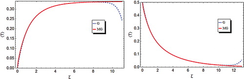
Fig. 1a and b shows the average reflectivity 〈R〉 and transmissivity 〈T〉, respectively, versus the mean thickness $\overline{L}$ of the atmospheric medium for a scattering albedo ω = 0.95, and natural (unpolarized) transferred radiation (α* = 0) using the Gaussian and modified Gaussian probability distribution functions for the statistical parameter β = 0.25. It appears that the modified Gaussian probability function gives more stable set of averaged results, as predicted in our considerations.

Fig. 1 〈R〉 and 〈T〉 versus $\overline{L}$ for ω = 0.95, α* = 0 and β = 0.25 for κ = 0.

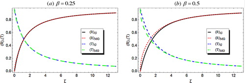
Fig. 2 shows the average reflectivity 〈R〉 and transmissivity 〈T〉 versus the mean thickness $\overline{L}$ at ω = 0.95, and for two different values of the statistical parameter β = 0.25 and β = 0.5 for the two polarization extremes (α* = ±1). As the statistical parameter β increases, differences appear between the Gaussian function and the modified Gaussian function. Hence, we use the modified Gaussian probability function for the remainder of the calculations.

Fig. 2 〈R〉 and 〈T〉 versus $\overline{L}$ for ω = 0.95, κ = 0 and α* = ±1.

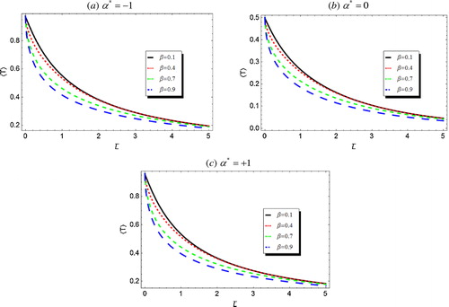
Figs. 3 and 4 show the average reflectivity 〈R〉 and transmissivity 〈T〉, respectively, versus the mean thickness $\overline{L}$ of the atmospheric medium for a scattering albedo ω = 0.9, at different degrees of polarization α* using four different values of the statistical parameter β. It is clear that the stochasticity of the random medium is very small for small thicknesses. However, for large media thicknesses, the difference between the results for different values of β disappear, i.e., as $\overline{L}\to \infty$, there no room for the medium randomness, according to the Gaussian statistical model.

Fig. 3 〈R〉 versus $\overline{L}$ for ω = 0.9 and κ = 0.

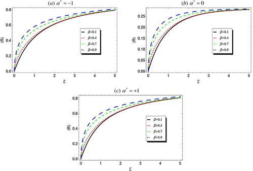
Fig. 4 〈T〉 versus $\overline{L}$ for ω = 0.9 and κ = 0.

6 Conclusions

In this work, we examined the stochastic transfer of polarized radiation in a random atmospheric finite medium. The atmospheric medium is considered to possess a continuous stochastic background (clouds or fog). The extinction function of the medium is assumed to be a continuous random function of position, with fluctuations occurring about the mean as being Gaussian distributed. The joint probability distribution function of these Gaussian random variables is used to calculate the averaged quantities, such as the average reflectivity and transmissivity over the medium fluctuations, for an arbitrary correlation function. The Pomraning–Eddington approximation is used to obtain the analytic deterministic solutions for the total intensity and the difference function of the polarized radiation. Then, the solution is averaged using the Gaussian probability distribution function. However, a modified Gaussian probability density function was used to overcome the defect associated with the usual Gaussian model. Numerical results were presented for both the average reflectivity and transmissivity at different polarization degrees α* and different values of the scattering albedo ω.

Using the modified Gaussian probability density provides more stable and smooth results (see Fig. 1), and disagreements between calculations performed using the Gaussian probability density function and the modified Gaussian probability density function appear for large values of the statistical parameter β (see Fig. 2b). Therefore, results were presented for the modified Gaussian probability density. The statistical random parameter β is more effective at calculating the average quantities, especially for intermediate thicknesses. In addition, it is crucial point to consider the polarization degree α* when calculating the transfer parameters of polarized radiation.

Acknowledgements

The authors would like to express their great thanks to Prof. Dr. S. A. El-Wakil for his encouragement and advice during this project.

Notes

Peer review under responsibility of Taibah University