Water body extraction and change detection using time series: A case study of Lake Burdur, Turkey

Peer review under responsibility of Taibah University.

Abstract

In this study, spatiotemporal changes in Lake Burdur from 1987 to 2011 were evaluated using multi-temporal Landsat TM and ETM+ images. Support Vector Machine (SVM) classification and spectral water indexing, including the Normalized Difference Water Index (NDWI), Modified NDWI (MNDWI) and Automated Water Extraction Index (AWEI), were used for extraction of surface water from image data. The spectral and spatial performance of each classifier was compared using Pearson's r, the Structural Similarity Index Measure (SSIM) and the Root Mean Square Error (RMSE). The accuracies of the SVM and satellite-derived indexes were tested using the RMSE. Overall, SVM followed by the MNDWI, NDWI and AWEI yielded the best result among all the techniques in terms of their spectral and spatial quality.

Keywords:

• Support vector machine
• Normalized difference water index
• Modified NDWI
• Automated water extraction index
• Change detection

1 Introduction

Water body extraction is an important task in different disciplines, such as lake coastal zone management, coastline change and erosion monitoring, flood prediction and evaluation of water resources [1]. Timely monitoring of surface water and delivering data on the dynamics of surface water are essential for policy and decision-making processes [2]. In recent years, integration of remote sensing data with Geographic Information Systems (GIS) has been used in automatic or semiautomatic water body extraction and mapping [3]. [4] Automatically extracted shorelines from Landsat TM and ETM+ multi-temporal images with subpixel precision techniques. [5] Developed an approach called the GeoCoverTM Water bodies Extraction Method that combines remote sensing and GIS to extract water bodies and study their abundance and morphometry. However, automatic coastline extraction is a complex process due to water saturated land transition zones at the land-water boundary [6,7]. To determine the spatially accurate coastline position, two methods have been explored: image classification and spectral water indexing. Multi-class support vector machine (SVM) classification for water body extraction and coastline detection has been commonly used by many researchers because it successfully minimizes errors and maximizes the geometric characteristics of edge areas [8,9]. Additionally, it has shown considerable potential in the supervised classification of remotely sensed data, requiring very limited training [10]. However, several water-indexing methods for the extraction of water bodies from remotely sensed data have been introduced by researchers. [11] Introduced the Normalized Difference Water Index (NDWI) to extract water features from Landsat TM using band 2 and band 4. [12] Introduced another NDWI for water extraction from Landsat TM using bands 3 and 5. [11] Proposed a threshold value of zero to extract surface water bodies from the raw digital Landsat values, where all positive NDWI values were classified as water and negative values as non-water. However, this threshold does not enable discrimination between built-up surfaces and water pixels. Thus, [13] introduced the Modified Normalized Difference Water (MNDWI) for Landsat TM using bands 2 and 5. [14] Introduced the Automated Water Extraction Index (AWEI) to improve water extraction accuracy in areas that include shadows and dark surfaces. [15] Introduced a simple Enhanced Water Index (EWI) based on the Modified Normalized Difference Water Index (MNDWI). It can effectively distinguish water surfaces from background information such as desert, soil and vegetation. [16] Investigated NDWI, MNDWI, NDMI, WRI, NDVI, and AWEI for the extraction of surface water from Landsat data and used a novel surface water change detection process based on the principal components of multi-temporal NDWI. In the study, surface water was extracted from the indexes using the thresholding technique based on the trial and error method. The performance of each water body extraction process was tested using the overall accuracy and kappa coefficient, and NDWI was found superior to other indexes. These indexes have also been previously tested in several applications, including surface water mapping [17,14], land use and land cover change analyses [18] and ecological research [19].

In this study, water body extraction techniques were applied to Lake Burdur to determine decreasing trends in the lake surface area in specified time intervals. The study focuses on the performance of each satellite-derived index and SVM classification. The spectral and spatial performances of the applied satellite-derived indexes and SVM were evaluated with Pearson's r and the Structural Similarity Index Measure (SSIM). In the literature, many studies were performed to extract water bodies based on satellite-derived indexes and evaluate the effectiveness of the satellite-derived indexes. Until now there have been no spatial performance analysis applied to satellite-derived indexes based on SSIM. Our study contributes to the effectiveness of the SSIM-based quality evaluation of satellite-derived indexes. The SSIM analysis provides a simple quantitative interpretation by comparing the correlations of luminance, contrast and structure locally between images and averaging these quantities over the entire image.

Lake Burdur, which is located in SW Turkey, has shrunk abruptly in recent decades. Therefore, regular and reliable measurements of the lake area are necessary to monitor the dynamic changes of lake water area for water resource balance analysis. Previous studies of the lake area were based on visual interpretation and manual digitization of satellite data [20,21]. In this study, the spatiotemporal changes of Lake Burdur from 1987 to 2011 are investigated based on SVM classification and satellite-derived water body extraction indexes, including NDWI, MNDWI and AWEI using Landsat TM and ETM+ data. The performances of the applied indexes were tested using Pearson's r, the SSIM and the Root Mean Square Error (RMSE). Overall, the SVM and NDWI were found superior to other indexes. The approach is highly significant for time-series analyses of extracted shorelines using any number of Landsat satellite images taken in different time intervals, and it provides an important comparison that can be used to investigate shoreline changes.

2 The study area and data

Lake Burdur is located in southwest Turkey (Fig. 1a, b). The southern part of the lake is bound by the tectonically active Burdur fault zone. Tectonically influenced half graben morphology controls the amount and type of sediment supply and turbidite systems of the lake [21].

Fig. 1 Location of Lake Burdur (Landsat TM 1987 false colour composites 4/3/2).

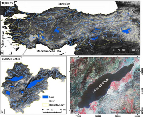
The image data used in this study were taken from 28 August 1987 for Landsat TM, 1 August 2000 for ETM+ and 19 August 2011 for Landsat TM+ (path 179, row 034). The sub-scenes of the data were all free of clouds, except Landsat TM-2011.

For accuracy, high spatial resolution Google Earth images were used for reference. The acquisition dates of the Google Earth reference data and Landsat TM and ETM images were matched to minimize errors in the lake surface water.

3 Methodology

The histograms of TM images display a board range of grey levels and display two different peaks for land and water areas. Based on the histogram observations, images were classified using the SVM and two classes to differentiate the land–water boundary. In the spectral water indexing process, a single number was derived from two or more spectral bands using an arithmetic operation. Based on the spectral characteristics, a suitable threshold of the index was then applied to image data to separate these two classes from each other. The pixels representing the coastline were converted into a vector layer to determine the coastline boundary and enable calculations of the area and perimeter of the lake. The performance of each satellite-derived index classifier was compared with those of other classifiers using CC and the SSIM. The accuracies of the SVM and satellite-derived index method were tested based on the RMSE.

3.1 Support Vector Machine classification

SVM is a supervised learning system and is based on recent improvements in statistical learning theory [22]. [23] Developed an SVM for binary classification. A number of studies have focused on the mathematical formulation of SVMs [23,24].

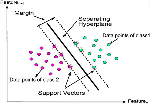
An SVM splits classes with a decision surface that maximizes the boundaries between the classes. The surface is called the ideal hyperplane, and the data points closest to the hyperplane are deemed support vectors (Fig. 2). The support vectors are the important elements of the training set [25,23,26].

Fig. 2 Linear support vector machine example (modified from Burges (1998)).

To execute an SVM, training data are needed. These data optimize the separation of the classes rather than describing the classes themselves [27]. Using a Radial Basis Function (RBF), class distributions with non-linear boundaries can be mapped in a high dimensional space for linear separation [28]. Training the SVM with a Gaussian RBF requires setting two parameters: a regularization parameter that controls the trade-off between maximizing the margin and minimizing the training error and kernel width. A small regularization parameter tends to emphasize the margin and ignore the outliers in the training data. A large regularization parameter may overfit the training data. A comprehensive description of the SVM parameters can be found in [24,22].

An SVM classifier includes four different types of kernels: linear, polynomial, RBF and sigmoid. The RBF kernel works fine in most cases [29]. The mathematical illustration of each kernel is listed in Eqs. (1)–(4):(1) $\text{Linear}:K(x_i,x_j)=x_i^t,x_j$(1) (2) $\text{Polynomial}:K(x_i,x_j)={(\gamma x_i^t{x}_j+r)}^d,\gamma >0$(2) (3) $\text{RBF}:K(x_i,x_j)=\exp (-\gamma ||x_i-x_j|{|}^2),\gamma >0$(3) (4) $\text{Sigmoid}:K(x_i,x_j)=\tanh (\gamma x_i^t{x}_j+r)$(4) where x_i is ith support vector; x_j is the jth training data point; t is the smoothing parameter; K is the kernel function; || is the Euclidean norm; γ is kernel width in the kernel functions of all kernel types, except the linear kernel; d is the polynomial degree term in the kernel function of the polynomial kernel; r is the bias term in the kernel functions of the polynomial and sigmoid kernels; and γ, d and r are user controlled parameters, as their correct definition significantly increases the SVM accuracy.

3.2 Spectral water indexes

Automatic coastline delineation is a complicated process due to the presence of the water-saturated zone at the land–water boundary [6,7]. Several spectral water indexes have been developed to extract water bodies from remotely sensed imagery, usually by calculating the normalized difference between two image bands and then applying an appropriate threshold to segment the results into two classes (water and non-water features). In this study, satellite imagery-derived NDWI, MNDWI and AWEI are used to extract lake water bodies from TM and ETM images.

3.2.1 Normalized Difference Water Index (NDWI)

The Normalized Difference Water Index (NDWI) was first suggested by [11] to detect surface waters in wetland environments and measure surface water dimensions. The NDWI for TM and ETM sensors is defined by Eq. (5)(5) $NDWI=\frac{ban{d}_2-ban{d}_4}{ban{d}_2+ban{d}_4}$(5) .(5) $NDWI=\frac{ban{d}_2-ban{d}_4}{ban{d}_2+ban{d}_4}$(5) As a result, water features have positive values and are enhanced. Vegetation and soil features usually have zero or negative values and are suppressed [11].

3.2.2 Modified Difference Water Index (MNDWI)

The MNDWI method suggested by [13] has been commonly used and is a powerful index that can extract water bodies [30,31]. It is expressed by Eq. (6)(6) $MNDWI=\frac{ban{d}_2-ban{d}_5}{ban{d}_2+ban{d}_5}$(6) .(6) $MNDWI=\frac{ban{d}_2-ban{d}_5}{ban{d}_2+ban{d}_5}$(6)

The resulting values representing the water features have positive values because of their higher reflectance in band 2 than in band 5, and non-water features have negative NDWI values [13]. A threshold value for MNDWI (e.g., simply a value of zero) can be set to segment the MNDWI results into two classes (water and non-water features).

3.2.3 Automated Water Extraction Index (AWEI)

The main aim of the AWEI is to maximize the separability of water and non-water pixels using band differencing, addition and application of different coefficients. Accordingly, two separate equations are proposed to effectively suppress non-water pixels and extract surface water with improved accuracy [14]. The mathematical definition of AWEI is given in Eqs. (7)(7) $AWE{I}_{nsh}=4x(\rho ban{d}_2-\rho ban{d}_5)-(0.25x\rho ban{d}_4+2.75x\rho ban{d}_7)$(7) and (8)(8) $AWE{I}_{sh}=\rho band{}_1+2.5x\rho ban{d}_2-1.5x(\rho ban{d}_4+\rho ban{d}_5)-0.25x\rho ban{d}_7$(8) :(7) $AWE{I}_{nsh}=4x(\rho ban{d}_2-\rho ban{d}_5)-(0.25x\rho ban{d}_4+2.75x\rho ban{d}_7)$(7) (8) $AWE{I}_{sh}=\rho band{}_1+2.5x\rho ban{d}_2-1.5x(\rho ban{d}_4+\rho ban{d}_5)-0.25x\rho ban{d}_7$(8) where ρ variables are the reflectance values of spectral bands of Landsat 5 TM: band 1, band 2, band 4, band 5 and band 7. AWEI_nsh is formulated to effectively eliminate non-water pixels, including dark, built-up surfaces in areas with urban backgrounds, and AWEI_sh further improves the accuracy by removing shadow pixels that AWEI_nsh may not effectively eliminate [14].

3.3 Performance evaluations of spectral water indexes

In this study, the performances of spectral water indexes for water body extraction were tested using Pearson's r and the SSIM.

3.3.1 Performance evaluation using Pearson's r

Pearson's r is a statistical measure of the strength and direction of a linear association between two images. The Pearson's r value between two images is defined in Eq. (9)(9) $r(A,B)=\frac{{\sum }_{m,n}(A_{m,n}-{\mu }_A)(B_{m,n}-{\mu }_B)}{\sqrt{{\sum }_{m,n}{(A_{m,n}-{\mu }_A)}^2{\sum B_{m,n}-{\mu }_B)}^2}}$(9) :(9) $r(A,B)=\frac{{\sum }_{m,n}(A_{m,n}-{\mu }_A)(B_{m,n}-{\mu }_B)}{\sqrt{{\sum }_{m,n}{(A_{m,n}-{\mu }_A)}^2{\sum B_{m,n}-{\mu }_B)}^2}}$(9) where μ_A and μ_B are the mean values of the two images (A and B), respectively. Pearson's r should be as close to one as possible. The difference between Pearson's r values will show how well the spatial quality is maintained [32].

3.3.2 Performance evaluation using the Structural Similarity Index Measure

The SSIM determines the similarity between two images by comparing the correlations of luminance, contrast and structure locally between the images and averaging these quantities over the entire image.

The luminance between the two signals is determined using the mean intensity of the signals given in Eq. (10)(10) $l(x,y)=\frac{2{\mu }_x{\mu }_y+C_1}{{\mu }_x^2+{\mu }_y^2+C_1}$(10) . The contrast is determined using the standard deviation presented in Eq. (11)(11) $C(x,y)=\frac{2{\sigma }_x{\sigma }_y+C_2}{{\sigma }_x^2+{\sigma }_y^2+C_2}$(11) . Finally, the structure is determined using the correlation presented in Eq. (12)(12) $S(x,y)=\frac{{\sigma }_{xy}+C_3}{{\sigma }_x{\sigma }_y+C_3}$(12) . This index was proposed by [33]. The SSIM values vary from zero to one. Values close to one show the highest similarity to the original images.(10) $l(x,y)=\frac{2{\mu }_x{\mu }_y+C_1}{{\mu }_x^2+{\mu }_y^2+C_1}$(10) (11) $C(x,y)=\frac{2{\sigma }_x{\sigma }_y+C_2}{{\sigma }_x^2+{\sigma }_y^2+C_2}$(11) (12) $S(x,y)=\frac{{\sigma }_{xy}+C_3}{{\sigma }_x{\sigma }_y+C_3}$(12)

In Eqs. (10)–(12), μ_x and μ_y are the sample means of x and y, respectively; σ_x and σ_y represent the sample variances of x and y, respectively; and σ_xy is the sample correlation coefficient between x and y. x and y refer to local windows in images X and Y, respectively. Constants C₁, C₂ and C₃ are used to stabilize the algorithm when the denominators approach zero. The SSIM (x, y) is a multiplication of these three components, as presented in Eq. (13)(13) $SSIM(x,y)=\frac{(2{\mu }_x{\mu }_y+C_1)x(2{\sigma }_{xy}+C_2)}{({\mu }_x^2+{\mu }_y^2+C_1)x({\sigma }_x^0+{\sigma }_y^2+C_2)}$(13) .(13) $SSIM(x,y)=\frac{(2{\mu }_x{\mu }_y+C_1)x(2{\sigma }_{xy}+C_2)}{({\mu }_x^2+{\mu }_y^2+C_1)x({\sigma }_x^0+{\sigma }_y^2+C_2)}$(13)

3.4 Validation of results using Root Mean Square Error

The RMSE is used to measure the difference between values predicted by a model and actual values. These individual differences are also called residuals, and the RMSE serves to aggregate them into a single measure of predictive power.

The RMSE of a model prediction with respect to the estimated variable X model is defined as the square root of the mean squared error (14)(14) $RMSE=\sqrt{\frac{{\sum }_{i=1}^n{(X_{obs,i}-X_{model,i})}^2}{n}}$(14) :(14) $RMSE=\sqrt{\frac{{\sum }_{i=1}^n{(X_{obs,i}-X_{model,i})}^2}{n}}$(14) where X_obs,i represents the observed values of the ith observation and X_model,i represents the predicted values at location i.

4 Results and analysis

4.1 Water body extraction using SVM

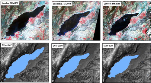
The image given below, which was acquired using the Landsat satellite (Fig. 3a–c), shows the changes in the lake from 1987 to 2011. These images were classified into two classes: water and land. The classification training samples were collected randomly from the representative homogeneous areas. The RBF was selected as the kernel method for SVM classification. This function works well in most cases and can handle linearly non-separable problems [29]. γ was determined as the inverse of the number of bands in the input image, and 1000 was taken as the value of the regularization parameter. After SVM classification, non-water areas were masked from the resultant images because the study focuses on water body areas (Fig. 3d–f).

Fig. 3 LANDSAT TM image from 1987 (a); LANDSAT-7 ETM+ image from 2000 (b); LANDSAT TM image from 2011; SVM-based extracted water body from the 1987 LANDSAT TM image (d), LANDSAT-7 ETM+ image from 2000 (e); LANDSAT TM image from 2011 (f).

4.2 Water body extraction using spectral water indexes

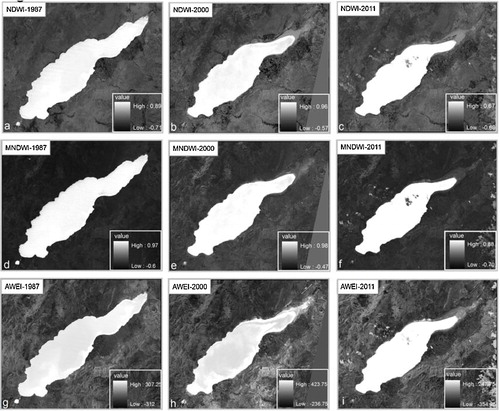
The three spectral water indexes (NDWI, MNDWI and AWEI) are applied to the lake water area to highlight the differences between water and non-water areas (Fig. 4a–i). The NDWI separates water and non-water objects well, with water areas generally having values greater than zero and vegetation areas having strong negative values. The NDWI and MNDWI images are classified into water and non-water using a threshold of zero [11]. The RMSE of the AWEI depends on the applied threshold value. The optimal threshold value for the AWEI, as recommended by [14], varies from −0.15 to 0.045. In this study, the threshold value was set to zero to provide consistency between all applied indexes.

Fig. 4 Image-derived spectral water indexes of the (a–c) NDWI; (d–f) MNDWI; and (g–i) AWEI for Lake Burdur.

4.3 Testing performance of shoreline extraction

4.3.1 Pearson's r

The spectral qualities of the indexes were measured with Pearson's r, as depicted in Table 1. The best correlation between the indexes shows the highest Pearson's r value. The highest Pearson's r was observed between the NDWI and MNDWI in 1987, 2000 and 2011, with values of 0.96, 0.91 and 0.96, respectively. The lowest Pearson's r values were observed between the NDWI and AWEI in 1987, 2000 and 2011, with values of 0.94, 0.90 and 0.87, respectively.

Table 1 Pearson's r between the NDWI, MNDWI and AWEI in 1987, 2000 and 2011.

	Pearson's r in 1987			Pearson's r in 2000			Pearson's r in 2011
	NDWI	MNDWI	AWEI	NDWI	MNDWI	AWEI	NDWI	MNDWI	AWEI
NDWI	1	0.96	0.94	1	0.91	0.90	1	0.96	0.87
MNDWI	–	1	0.95	–	1	0.91	–	1	0.93
AWEI	–	–	1	–	–	1	–	–	1

4.3.2 Structural Similarity Index (SSIM)

The structural similarity among spectral water indexing was measured with SSIM. Values close to one show the highest similarity between indexes. All the applied indexes had SSIM values higher than 82%, verifying the fact that there was high similarity among the applied water indexes. As seen in Table 2, the SSIM rate indicates that the NDWI and MNDWI provide the highest structural similarities, with values of 96%, 87% and 95% in 1987, 2000 and 2011, respectively. The SSIM was the lowest between NDWI and AWEI, with values of 96%, 82% and 94% in 1987, 2000 and 2011, respectively. The differences between the applied indexes are given in Fig. 5. In this figure, white pixels represent no difference and black pixels indicate maximum difference.

Fig. 5 SSIM map of the spectral water indexes derived from a LANDSAT TM image from 1987 (a–c); LANDSAT-7 ETM+ image from 2000 (d–f); LANDSAT TM image from 2011 (g–i).

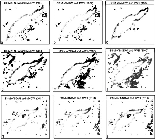
Table 2 SSIM between the NDWI, MNDWI and AWEI in 1987, 2000 and 2011.

	SSIM in 1987			SSIM in 2000			SSIM in 2011
	NDWI	MNDWI	AWEI	NDWI	MNDWI	AWEI	NDWI	MNDWI	AWEI
NDWI	1	0.96	0.96	1	0.87	0.82	1	0.95	0.94
MNDWI		1	0.99		1	0.85		1	0.94
AWEI			1			1			1

4.3.3 Geometric accuracy assessment and comparison

To compare the derived lake water surface areas, the lake water area was digitized manually on-screen from the Landsat images. High-resolution Google Earth images were used as references to help differentiate confusing water pixels from background features. Many of the pixel values of land and water areas were mixed near the lake shoreline. To compare the Landsat data with data obtained from Google Earth, image-to-image registration was performed to geometrically align two images. The image-derived coastlines were compared to reference data, which was produced by manually digitizing the lake perimeter using the Landsat images and Google Earth images. The RMSE was calculated using the reference data, as shown in Table 3. The accuracies achieved by the SVM and MNDWI in 1987, 2000 and 2011 are higher than those of the NDWI and AWEI classifiers. For the SVM classifier, the RMSE ranges between 33.14 m and 50.48 m. For the NDWI classifier, the RMSE ranges between 51.94 m and 61.62 m. The water body was extracted from satellite images with a 30 m spatial resolution. Therefore, these errors correspond to approximately one and two pixels in the satellite image.

Table 3 RMSE between reference data and image-derived shorelines.

	SWM	NDWI	MNDWI	AWEI
RMSE (m) 1987	50.48	61.62	45.67	64.36
RMSE (m) 2000	33.14	51.94	50.44	109.81
RMSE (m) 2011	48.16	55.77	45.99	60.95

4.3.4 Evaluation of the change

The lake water area was extracted using SVM classification and spectral water indexing in 1987–2000 and 2011, as shown in Fig. 6. The shoreline shrunk in the twenty-four year span of images. According to the SVM, NDWI, MNWI and AWEI, between 1987 and 2000 there were dramatic changes in lake water area, and the changes between 2000 and 2011 were compared. The SVM, NDWI, MNWI and AWEI results reveal that the surface area of Lake Burdur in August 1987 was approximately 203 km² (Table 4). By August 2000, based on the NDWI and MNWI, the surface area had decreased to approximately 157 km². From 1987 to 2000, the lake lost about one fifth of its surface area compared to that in 1987. However, from 2000 to 2011, the lake lost about one tenth of its surface area compared to that in 2000 (Table 4). According to the results given in Fig. 6a–d, the highest rate of water area change was observed in the NE part of the lake.

Fig. 6 Changes in the area of Lake Burdur in 1987, 2000 and 2011 generated using (a) SVM; (b) NDWI; (c) MNDWI; (d) AWEI.

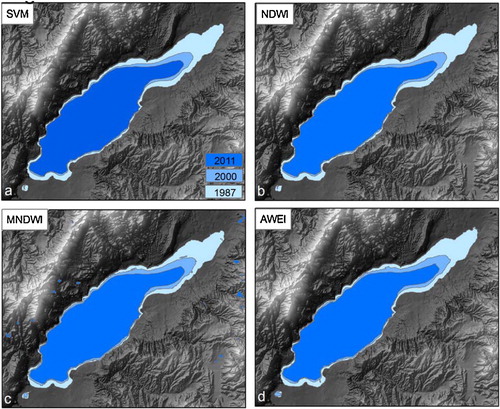
Table 4 Water body area change of Lake Burdur in 1987, 2000 and 2011.

	SVM	NDWI	MNDWI	AWEI
Area in 1987 (km^2)	203.55	203.10	203.17	203.59
Area in 2000 (km^2)	156.19	157.12	157.49	161.76
Area in 2011 (km^2)	142.18	141.40	141.68	142.32
Change 1987–2000 (%)	23.27	22.64	22.48	20.55
Change 2000–2011 (%)	8.97	10.01	10.04	12.02
Total change 1987–2011 (%)	32.24	32.65	32.52	32.57

5 Discussion

Water body extraction accuracy problems may be particularly noticeable in areas where the background land cover includes low albedo surfaces (e.g., buildings, asphalts, shadows and clouds). The presence of shadows in the images may cause misclassification due to similar spectral reflectance patterns as water body areas, and this similarity may decrease the accuracy of extracted surface water areas and vary the analysis between specified time intervals [13,3,34]. In environments with low spectral reflectance where non-water dark surfaces are found, simple classification methods may not adequately and accurately distinguish water pixels from non-water pixels, particularly in shadows [34]. Thus, three different spectral water indexes were used in this study. In the NDWI, MNDWI and AWEI images, slight differences cannot be manually detected by visual inspection. Therefore, Pearson's r and SSIM are measured among the three indexes. The SSIM analysis provides a simple quantitative interpretation by comparing the correlations between luminance, contrast and structure locally between the images and averaging these quantities over the entire image. The major advantage of SSIM is that it is a simple and straightforward method for comparing two or more maps. The results reveal that SSIM and Pearson's r provide quality scores that are correlated to RMSE values.

The results of the applied methodology suggest that no existing water index was able to automatically differentiate water surfaces from shadow surfaces and low albedo urban surfaces. The MNDWI is more appropriate for differentiating water in many built-up areas compared to using NDWI. The applied threshold values of the MNDWI used to obtain the best water extraction outcome are usually much less than those of the NDWI. Using zero as a default threshold value can produce better water body separation accuracy using the MNDWI. This would be very useful for more accurately extraction of water bodies from image data using the MNDWI. Additionally, the MNDWI gives more detailed information regarding open water than does the NDWI. This property is also useful for the detection of water quality differences in specified time intervals.

The most critical aspect of the applied method is the accuracy assessment. For the accuracy test, a reference lake water area was digitized manually on-screen from the Landsat images. This step is totally user-dependent and subjective. The literature suggests that the accuracy of the reference map is directly related to the experience of the user. The advantage of the extraction processes in this study is that the study area is well known by the authors, who are familiar with the lake morphology of the area.

6 Conclusions

This study used satellite image interpretation and GIS to detect and analyze the spatial changes and quantify the water area change of Lake Burdur. Using satellite images to extract information regarding lake water area change is faster and more accurate than other observation methods, particularly in identifying changes between two and three different time intervals. The approach is based on SVM classification and spectral water indexing (NDWI, MDWI and AWEI). According to the results of Pearson's r, the SSIM and RMSE of the SVM classification and spectral water indexing, SVM and NDWI performed significantly better than did other indexes for mapping the lake water surface using Landsat data.

Depending on these outcomes, from 1987 to 2000, the lake lost about one fifth of its surface area, as compared to the surface area in 1987. From 2000 to 2011, the lake lost about one tenth of its surface area compared to that in 2000. This study demonstrated the feasibility of estimating lake water area variations using only freely available satellite data.

Acknowledgements

The authors would like to thank the anonymous reviewers for their helpful and constructive feedback.

Notes

Peer review under responsibility of Taibah University.