Extended G′G -expansion method for Calogero–Bogoyavlinskii–Schiff equation of fractional order

Peer review under responsibility of Taibah University.

Abstract

In this paper, we explore new applications of the extended $\left(\frac{G^{\prime }}{G}\right)\text{-expansion}$ method. We apply this method to the nonlinear Calogero–Bogoyavlinskii–Schiff equation of fractional order. As results, some new exact traveling wave solutions are obtained which include solitary wave solutions. The traveling wave solutions are expressed by hyperbolic and trigonometric functions.

Keywords:

• Fractional derivative
• The extended $\left(\frac{G^{\prime }}{G}\right)\text{-expansion}$ method
• Calogero–Bogoyavlinskii–Schiff equation
• Traveling wave solutions

1 Introduction

In the recent years, the exact solutions of nonlinear partial differential equations (NLPDEs) have been investigated by many authors who are interested in nonlinear phenomena which exist in all fields including either the scientific works or engineering fields, such as fluid mechanics, chemical physics, chemical kinematics, plasma physics, elastic media, optical fibers, solid state physics, biology, atmospheric and oceanic phenomena and so on. The research of traveling wave solutions of some nonlinear evolution equations derived from such fields played an important role in the analysis of some phenomena. To obtain traveling wave solutions, many effective methods have been presented in the literature, such that the homogeneous balance method [1,2], the hyperbolic tangent expansion method [3,4], the trial function method [5], the tanh-function method [6–9], the theta function method [10–12], the nonlinear transform method [13], the Hirota bilinear method [14,15], the Weierstrass elliptic function method [16], the F-function expansion method [17–19], the inverse scattering transform [20], the exp-function expansion method [21], the Jacobi elliptic function expansion [2,11,22–26], the Backlund transform method [27,28], the generalized Riccati equation method [29], the original $\left(\frac{G^{\prime }}{G}\right)\text{-expansion}$ method [30], the sub-ODE method [30,31,32,33], and so on. Recently, Wang et al. [30] first introduced the expansion method to look for traveling wave solutions of nonlinear evolution equations. By means of this method, Wang et al. [30] and other authors obtained more traveling wave solutions of different NLPDEs. More recently, Guo and Zhou [34] first proposed the extended $\left(\frac{G^{\prime }}{G}\right)\text{-expansion}$ method based on new ansatze. Theyapplied this method to the Whitham–Broer–Kaup-Like equations and coupled Hirota–Satsuma K dV equation. Recently, Zayed et al. [35] have applied the extended $\left(\frac{G^{\prime }}{G}\right)\text{-expansion}$ method to some different nonlinear PDEs and found the exact traveling wave solutions. The objective of the present work is to apply the extended $\left(\frac{G^{\prime }}{G}\right)\text{-expansion}$ method which has been proposed by Hayek [36] for the nonlinear Calogero–Bogoyavlinskii–Schiff equation of fractional order.

2 Preliminaries and notations

We give some basic definitions and properties of the fractional calculus theory which are used further in this paper.

2.1 Definition

A real function f(t), t > 0, is said to be in the space c_μ, μ ∈ R if there exists a real number p(>μ), such that f(t) = t^pf₁(t), where f₁(t) ∈ C[0, ∞], and it is said to be in the space $C_{\mu }^m$ iff f^m ∈ C_μ, m ∈ N.

2.2 Definition

The Riemann–Liouville fractional integral operator of order α ≥ 0, of a function f ∈ C_μ, μ ≥−1, is defined as$J^{\alpha }f(t)=\frac{1}{\Gamma (\alpha )}{\int }_0^t{(t-\tau )}^{\alpha -1}f(\tau )d\tau ,\alpha >0,t>0,$$J^{0}f(t)=f(t)\text{,}$properties of the operator J^α can be found in [37–39], we mention only the following: For f ∈ C_μ, μ ≥−1, α, β ≥ 0 and γ >−1:

1.	JαJβf(t) = Jα+βf(t).

2.	JαJβf(t) = JβJαf(t).

3.	$J^{\alpha }{t}^{\gamma }=\frac{\Gamma (\gamma +1)}{\Gamma (\alpha +\gamma +1)}{t}^{\alpha +\gamma }\text{.}$

The Riemann–Liouville derivative has certain disadvantages when trying to model real-world phenomena with fractional differential equations. Therefore, we shall introduce a modified fractional differential operator D^α proposed by Caputo in his work on the theory of viscoelasticity [40].

2.3 Definition

The fractional derivative of f(t) in the Caputo sense is defined as$D^{\alpha }f(t)=J^{m-\alpha }{D}^{m}f(t)=\frac{1}{\Gamma (m-\alpha )}{\int }_0^t{(t-\tau )}^{m-\alpha -1}{f}^m(t)dt\text{,}$for $m-1<\alpha \le 1m,m\in N,t>0,f\in C_{-1}^m$.

3 Description of the extended $\left(\frac{G^{\prime }}{G}\right)\text{-expansion}$ method

Suppose we have the following nonlinear PDE of the type(3.1) $P(u,u_t,u_x,u_z,u_{tt},u_{xx},u_{zz},u_{xy},\dots )=0\text{,}$(3.1) where u(ξ) = u(x, z, t) is an unknown function, P is a polynomial in u = u(x, z, t) and its various partial derivatives, in which the highest order partial derivatives and the nonlinear terms are involved.

In the following, we give the main steps of the extended $\left(\frac{G^{\prime }}{G}\right)\text{-expansion}$ method [34–36]:

Step 1:

Combining the independent variables x, z and t into one variable ξ, we suppose that(3.2) $u(x,z,t)=u(\xi ),\xi =x+z\pm \omega \frac{t^{\alpha }}{\Gamma (\alpha +1)}\text{,}$(3.2) where ω is the speed of the traveling wave, permits us to transform the Eq. (3.1)(3.1) $P(u,u_t,u_x,u_z,u_{tt},u_{xx},u_{zz},u_{xy},\dots )=0\text{,}$(3.1) into an ODE:(3.3) $Q(u,u^{\prime },u^{″},u^{‴},\dots )=0\text{,}$(3.3) where the superscripts stands for the ordinary derivatives with respect to ξ.

Step 2:

If possible, integrate Eq. (3.3)(3.3) $Q(u,u^{\prime },u^{″},u^{‴},\dots )=0\text{,}$(3.3) term by term one or more times. This yields constant(s) of integration.

Step 3:

Suppose the traveling wave solution of Eq. (3.3)(3.3) $Q(u,u^{\prime },u^{″},u^{‴},\dots )=0\text{,}$(3.3) can be expressed by a polynomial in G as follows: (3.4) $u(\xi )=a_0+\sum _{i=1}^m\left\{a_i{\left(\frac{G^{\prime }}{G}\right)}^i+b_i{\left(\frac{G^{\prime }}{G}\right)}^{i-1}\sqrt{\sigma \left(1+\frac{1}{\mu }{\left(\frac{G^{\prime }}{G}\right)}^2\right)}\right\}+\sum _{i=1}^m\left\{c_i{\left(\frac{G^{\prime }}{G}\right)}^{-i}+d_i\frac{{\left(\frac{G\text{'}}{G}\right)}^{-i+1}}{\sqrt{\sigma \left(1+\frac{1}{\mu }{\left(\frac{G\text{'}}{G}\right)}^2\right)}}\right\}\text{,}$(3.4) where G = G(ξ) satisfy the first order nonlinear ODE in the form,(3.5) $G^{″}+\mu G=0\text{,}$(3.5) and μ is a nonzero constant. The coefficients a0, ai, bi, ci, di (i = 1, …, m) are arbitrary constants to be determined later, and σ =±1, while m is a positive integer.

Step 4:

The positive integer m can be determined by considering the homogeneous balance between the highest order derivatives and the nonlinear terms appearing in Eq. (3.3)(3.3) $Q(u,u^{\prime },u^{″},u^{‴},\dots )=0\text{,}$(3.3) . Moreover precisely, we define the degree of u(ξ) as D[u(ξ)] = m which gives rise to the degree of other expression as follows:(3.6) $D\left(\frac{d^{q}u}{d{\xi }^q}\right)=m+q,D\left(u^p{\left(\frac{d^{q}u}{d{\xi }^q}\right)}^s\right)=mp+s(m+q)\text{.}$(3.6) Therefore, we can find the value of m. in Eq. (3.4)(3.4) $u(\xi )=a_0+\sum _{i=1}^m\left\{a_i{\left(\frac{G^{\prime }}{G}\right)}^i+b_i{\left(\frac{G^{\prime }}{G}\right)}^{i-1}\sqrt{\sigma \left(1+\frac{1}{\mu }{\left(\frac{G^{\prime }}{G}\right)}^2\right)}\right\}+\sum _{i=1}^m\left\{c_i{\left(\frac{G^{\prime }}{G}\right)}^{-i}+d_i\frac{{\left(\frac{G\text{'}}{G}\right)}^{-i+1}}{\sqrt{\sigma \left(1+\frac{1}{\mu }{\left(\frac{G\text{'}}{G}\right)}^2\right)}}\right\}\text{,}$(3.4) , using Eq. (3.6)(3.6) $D\left(\frac{d^{q}u}{d{\xi }^q}\right)=m+q,D\left(u^p{\left(\frac{d^{q}u}{d{\xi }^q}\right)}^s\right)=mp+s(m+q)\text{.}$(3.6) .

Step 5:

We substitute Eq. (3.4)(3.4) $u(\xi )=a_0+\sum _{i=1}^m\left\{a_i{\left(\frac{G^{\prime }}{G}\right)}^i+b_i{\left(\frac{G^{\prime }}{G}\right)}^{i-1}\sqrt{\sigma \left(1+\frac{1}{\mu }{\left(\frac{G^{\prime }}{G}\right)}^2\right)}\right\}+\sum _{i=1}^m\left\{c_i{\left(\frac{G^{\prime }}{G}\right)}^{-i}+d_i\frac{{\left(\frac{G\text{'}}{G}\right)}^{-i+1}}{\sqrt{\sigma \left(1+\frac{1}{\mu }{\left(\frac{G\text{'}}{G}\right)}^2\right)}}\right\}\text{,}$(3.4) into Eq. (3.3)(3.3) $Q(u,u^{\prime },u^{″},u^{‴},\dots )=0\text{,}$(3.3) using the LODE (3.5)(3.5) $G^{″}+\mu G=0\text{,}$(3.5) and then collect all terms with the same order of ${\left(\frac{G^{\prime }}{G}\right)}^k\text{and}{\left(\frac{G^{\prime }}{G}\right)}^k\sqrt{\sigma \left(1+\frac{1}{\mu }{\left(\frac{G^{\prime }}{G}\right)}^2\right)}\text{,}$ we get a polynomial. Equating each coefficient of this polynomial to zero, yields a set of algebraic equations, which can be solved to get the values of ω, μ, a0, ai, bi, ci, di.

Step 6:

Since the general solution of Eq. (3.5)(3.5) $G^{″}+\mu G=0\text{,}$(3.5) is well known to us, then substituting the values of ω, μ, a0, ai, bi, ci, di and the general solutions of (3.5)(3.5) $G^{″}+\mu G=0\text{,}$(3.5) into (3.4)(3.4) $u(\xi )=a_0+\sum _{i=1}^m\left\{a_i{\left(\frac{G^{\prime }}{G}\right)}^i+b_i{\left(\frac{G^{\prime }}{G}\right)}^{i-1}\sqrt{\sigma \left(1+\frac{1}{\mu }{\left(\frac{G^{\prime }}{G}\right)}^2\right)}\right\}+\sum _{i=1}^m\left\{c_i{\left(\frac{G^{\prime }}{G}\right)}^{-i}+d_i\frac{{\left(\frac{G\text{'}}{G}\right)}^{-i+1}}{\sqrt{\sigma \left(1+\frac{1}{\mu }{\left(\frac{G\text{'}}{G}\right)}^2\right)}}\right\}\text{,}$(3.4) , we have the traveling wave solutions of Eq. (3.1)(3.1) $P(u,u_t,u_x,u_z,u_{tt},u_{xx},u_{zz},u_{xy},\dots )=0\text{,}$(3.1) .

Remark 1

The nonzero parameter μ in Eq. (3.5)(3.5) $G^{″}+\mu G=0\text{,}$(3.5) plays an essential role in the determination of the type of the solutions. Indeed,

(i)	If μ < 0, then we find the hyperbolic-type solutions and we have(3.7) $\frac{G^{\prime }}{G}=\sqrt{-\mu }\left(\frac{A_1\text{sinh}(\sqrt{-\mu }\xi )+A_2\text{cosh}(\sqrt{-\mu }\xi )}{A_1\text{cosh}(\sqrt{-\mu }\xi )+A_2\text{sinh}(\sqrt{-\mu }\xi )}\right)\text{.}$(3.7)

(ii)

If μ > 0, then we find the trigonometric-type solutions and we have(3.8) $\frac{G^{\prime }}{G}=\sqrt{\mu }\left(\frac{A_1\text{cos}(\sqrt{\mu }\xi )-A_2\text{sin}(\sqrt{\mu }\xi )}{A_1\text{sin}(\sqrt{\mu }\xi )+A_2\text{cos}(\sqrt{\mu }\xi )}\right)\text{,}$(3.8) where A1 and A2 are arbitrary constants.

4 Applications

In this section, we apply the extended $\left(\frac{G^{\prime }}{G}\right)\text{-expansion}$ method to construct some new traveling wave solutions of thenonlinear Calogero–Bogoyavlinskii–Schiff equation of fractional order in mathematical physics which have been paid attention by many researchers. Inspired and motivated by the ongoing research in this area, we apply the extended $\left(\frac{G^{\prime }}{G}\right)\text{-expansion}$ method for searching its new solitary wave solutions. Let us consider the Calogero–Bogoyavlinskii–Schiff equation with fractional derivative(4.1) $D_t^{2\alpha }{u}_x+u_{xxxz}+4u_x{u}_{xz}+2u_{xx}{u}_z=0,0<\alpha <1$(4.1) Consider the following transformation to convert Eq. (4.1)(4.1) $D_t^{2\alpha }{u}_x+u_{xxxz}+4u_x{u}_{xz}+2u_{xx}{u}_z=0,0<\alpha <1$(4.1) into ordinary differential equation(4.2) $u(x,z,t)=u(\xi ),\xi =x+z+\omega \frac{t^{\alpha }}{\Gamma (\alpha +1)}\text{,}$(4.2) where ω is a real constant. Substituting Eq. (4.2)(4.2) $u(x,z,t)=u(\xi ),\xi =x+z+\omega \frac{t^{\alpha }}{\Gamma (\alpha +1)}\text{,}$(4.2) into Eq. (4.1)(4.1) $D_t^{2\alpha }{u}_x+u_{xxxz}+4u_x{u}_{xz}+2u_{xx}{u}_z=0,0<\alpha <1$(4.1) and using the chain rule, we obtained the following ODE(4.3) $\omega u^{″}+u^{iv}+6u^{\prime }{u}^{″}=0\text{.}$(4.3) Integrating Eq. (4.3)(4.3) $\omega u^{″}+u^{iv}+6u^{\prime }{u}^{″}=0\text{.}$(4.3) once with respect to ξ, we get(4.4) $C+\omega u^{\prime }+u^{‴}+3{(u^{\prime })}^2=0\text{,}$(4.4) where C is a constant of integration. Now balancing the term u‴ and ${(u^{\prime })}^2$, yields n = 1.

Hence for n = 1, Eq. (3.4)(3.4) $u(\xi )=a_0+\sum _{i=1}^m\left\{a_i{\left(\frac{G^{\prime }}{G}\right)}^i+b_i{\left(\frac{G^{\prime }}{G}\right)}^{i-1}\sqrt{\sigma \left(1+\frac{1}{\mu }{\left(\frac{G^{\prime }}{G}\right)}^2\right)}\right\}+\sum _{i=1}^m\left\{c_i{\left(\frac{G^{\prime }}{G}\right)}^{-i}+d_i\frac{{\left(\frac{G\text{'}}{G}\right)}^{-i+1}}{\sqrt{\sigma \left(1+\frac{1}{\mu }{\left(\frac{G\text{'}}{G}\right)}^2\right)}}\right\}\text{,}$(3.4) reduces to(4.5) $u(\xi )=a_0+a_1\left(\frac{G^{\prime }}{G}\right)+b_1\sqrt{\sigma \left(1+\frac{1}{\mu }{\left(\frac{G^{\prime }}{G}\right)}^2\right)}+c_1{\left(\frac{G^{\prime }}{G}\right)}^{-1}+d_1\frac{1}{\sqrt{\sigma \left(1+\frac{1}{\mu }{\left(\frac{G^{\prime }}{G}\right)}^2\right)}}\text{,}$(4.5) where a₀, a₁, b₁, c₁, d₁ are constants to be determined and G = G(ξ) satisfies Eq. (3.5)(3.5) $G^{″}+\mu G=0\text{,}$(3.5) .

Substituting Eq. (4.5)(4.5) $u(\xi )=a_0+a_1\left(\frac{G^{\prime }}{G}\right)+b_1\sqrt{\sigma \left(1+\frac{1}{\mu }{\left(\frac{G^{\prime }}{G}\right)}^2\right)}+c_1{\left(\frac{G^{\prime }}{G}\right)}^{-1}+d_1\frac{1}{\sqrt{\sigma \left(1+\frac{1}{\mu }{\left(\frac{G^{\prime }}{G}\right)}^2\right)}}\text{,}$(4.5) along with Eq. (3.5)(3.5) $G^{″}+\mu G=0\text{,}$(3.5) into Eq. (4.3)(4.3) $\omega u^{″}+u^{iv}+6u^{\prime }{u}^{″}=0\text{.}$(4.3) , we obtain a polynomial in ${\left(\frac{G^{\prime }}{G}\right)}^k\text{and}{\left(\frac{G^{\prime }}{G}\right)}^k\sqrt{\sigma \left(1+\frac{1}{\mu }{\left(\frac{G^{\prime }}{G}\right)}^2\right)}$. On equating the coefficients of this polynomial to zero, we get a system of algebraic equations as follows:(4.6) $\begin{array}{l}{\left(\frac{G^{\prime }}{G}\right)}^0:6{\mu }^5\sigma c_1+3{\mu }^4\sigma c_1^2=0,\hfill \\ {\left(\frac{G^{\prime }}{G}\right)}^2:-6{\mu }^4\sigma a_1{c}_1+{\mu }^3\omega \sigma c_1+14{\mu }^4\sigma c_1+9{\mu }^3\sigma c_1^2=0,\hfill \\ ⋮\hfill \\ {\left(\frac{G^{\prime }}{G}\right)}^8:-6\mu a{b}_1{d}_1-6\mu a{a}_1{c}_1+\mu \omega \sigma a_1+6\mu {\sigma }^2{b}_1^2-14{\mu }^2\sigma a_1+9{\mu }^2\sigma a_1^2=0,\hfill \\ {\left(\frac{G^{\prime }}{G}\right)}^3\sqrt{\sigma \left(1+\frac{1}{\mu }{\left(\frac{G^{\prime }}{G}\right)}^2\right)}:-6{\mu }^3\sigma b_1{c}_1+6{\mu }^3{c}_1{d}_1=0,\hfill \\ {\left(\frac{G^{\prime }}{G}\right)}^5\sqrt{\sigma \left(1+\frac{1}{\mu }{\left(\frac{G^{\prime }}{G}\right)}^2\right)}:6{\mu }^3\sigma a_1{b}_1-5{\mu }^3\sigma b_1-6{\mu }^3{a}_1{d}_1-{\mu }^2\omega \sigma b_1-12{\mu }^2\sigma b_1{c}_1-{\mu }^3{d}_1+{\mu }^2\omega d_1+6{\mu }^2{c}_1{d}_1=0,\hfill \\ ⋮\hfill \\ {\left(\frac{G^{\prime }}{G}\right)}^8\sqrt{\sigma \left(1+\frac{1}{\mu }{\left(\frac{G^{\prime }}{G}\right)}^2\right)}:-6\mu \sigma b_1{d}_1-6\mu \sigma a_1{c}_1-\mu \omega \sigma a_1+6\mu {\sigma }^2{b}_1^2-14{\mu }^2\sigma a_1+9{\mu }^2\sigma a_1^2=0.\hfill \end{array}$(4.6) On solving the above system of algebraic equations (4.6)(4.6) $\begin{array}{l}{\left(\frac{G^{\prime }}{G}\right)}^0:6{\mu }^5\sigma c_1+3{\mu }^4\sigma c_1^2=0,\hfill \\ {\left(\frac{G^{\prime }}{G}\right)}^2:-6{\mu }^4\sigma a_1{c}_1+{\mu }^3\omega \sigma c_1+14{\mu }^4\sigma c_1+9{\mu }^3\sigma c_1^2=0,\hfill \\ ⋮\hfill \\ {\left(\frac{G^{\prime }}{G}\right)}^8:-6\mu a{b}_1{d}_1-6\mu a{a}_1{c}_1+\mu \omega \sigma a_1+6\mu {\sigma }^2{b}_1^2-14{\mu }^2\sigma a_1+9{\mu }^2\sigma a_1^2=0,\hfill \\ {\left(\frac{G^{\prime }}{G}\right)}^3\sqrt{\sigma \left(1+\frac{1}{\mu }{\left(\frac{G^{\prime }}{G}\right)}^2\right)}:-6{\mu }^3\sigma b_1{c}_1+6{\mu }^3{c}_1{d}_1=0,\hfill \\ {\left(\frac{G^{\prime }}{G}\right)}^5\sqrt{\sigma \left(1+\frac{1}{\mu }{\left(\frac{G^{\prime }}{G}\right)}^2\right)}:6{\mu }^3\sigma a_1{b}_1-5{\mu }^3\sigma b_1-6{\mu }^3{a}_1{d}_1-{\mu }^2\omega \sigma b_1-12{\mu }^2\sigma b_1{c}_1-{\mu }^3{d}_1+{\mu }^2\omega d_1+6{\mu }^2{c}_1{d}_1=0,\hfill \\ ⋮\hfill \\ {\left(\frac{G^{\prime }}{G}\right)}^8\sqrt{\sigma \left(1+\frac{1}{\mu }{\left(\frac{G^{\prime }}{G}\right)}^2\right)}:-6\mu \sigma b_1{d}_1-6\mu \sigma a_1{c}_1-\mu \omega \sigma a_1+6\mu {\sigma }^2{b}_1^2-14{\mu }^2\sigma a_1+9{\mu }^2\sigma a_1^2=0.\hfill \end{array}$(4.6) by Maple 13, we obtain the following results:

Case 1:

$a_0=a_0,a_1=a_1,b_1=0,c_1=-\mu a_1,d_1=0,\omega =15\mu a_1-14\mu ,C=15{\mu }^2{a}_1^2-30{\mu }^2{a}_1\text{.}$

Case 2:

a0 = a0, a1 = 2, b1 = 0, c1 = 0, d1 = 0, ω = 4 µ, C = 0.

Case 3:

a0 = a0, a1 = 0, b1 = 0, c1 =−2 µ, d1 = 0, ω = 4 µ, C = 0.

Case 4:

a0 = a0, a1 = 1, b1 = b1, c1 =− µ, d1 = σb1, ω = µ, C =−15 µ 2.

Case 5:

$a_0=a_0,a_1=1,b_1=\sqrt{\frac{\mu }{\sigma }},c_1=0,d_1=0,\omega =\mu ,C=0\text{.}$

Case 6:

$a_0=a_0,a_1=1,b_1=\sqrt{\frac{\mu }{\sigma }},c_1=-\mu ,d_1=\frac{\mu }{\sqrt{\frac{\mu }{\sigma }}},\omega =\mu ,C=-15{\mu }^2\text{.}$

(a) Hyperbolic function solutions

Substituting (3.7)(3.7) $\frac{G^{\prime }}{G}=\sqrt{-\mu }\left(\frac{A_1\text{sinh}(\sqrt{-\mu }\xi )+A_2\text{cosh}(\sqrt{-\mu }\xi )}{A_1\text{cosh}(\sqrt{-\mu }\xi )+A_2\text{sinh}(\sqrt{-\mu }\xi )}\right)\text{.}$(3.7) into (4.5)(4.5) $u(\xi )=a_0+a_1\left(\frac{G^{\prime }}{G}\right)+b_1\sqrt{\sigma \left(1+\frac{1}{\mu }{\left(\frac{G^{\prime }}{G}\right)}^2\right)}+c_1{\left(\frac{G^{\prime }}{G}\right)}^{-1}+d_1\frac{1}{\sqrt{\sigma \left(1+\frac{1}{\mu }{\left(\frac{G^{\prime }}{G}\right)}^2\right)}}\text{,}$(4.5) , we get the following hyperbolic traveling wave solutions:

Case 1 gives(4.7) $u(\xi )=a_0+a_1\sqrt{-\mu }\left(\frac{A_1\text{sinh}(\sqrt{-\mu }\xi )+A_2\text{cosh}(\sqrt{-\mu }\xi )}{A_1\text{cosh}(\sqrt{-\mu }\xi )+A_2\text{sinh}(\sqrt{-\mu }\xi )}\right)-\frac{\mu a_1}{\sqrt{-\mu }}{\left[\frac{A_1\text{sinh}(\sqrt{-\mu }\xi )+A_2\text{cosh}(\sqrt{-\mu }\xi )}{A_1\text{cosh}(\sqrt{-\mu }\xi )+A_2\text{sinh}(\sqrt{-\mu }\xi )}\right]}^{-1}\text{,}$(4.7) where $\xi =x+z+\frac{(15\mu a_1-14\mu )t^{\alpha }}{\Gamma (\alpha +1)}\text{,}$ and μ, a₁ and a₀ are arbitrary constants.

Case 2 gives(4.8) $u(\xi )=a_0+2\sqrt{-\mu }\left(\frac{A_1\text{sinh}(\sqrt{-\mu }\xi )+A_2\text{cosh}(\sqrt{-\mu }\xi )}{A_1\text{cosh}(\sqrt{-\mu }\xi )+A_2\text{sinh}(\sqrt{-\mu }\xi )}\right)\text{,}$(4.8) where $\xi =x+z+\frac{4\mu t^{\alpha }}{\Gamma (\alpha +1)}$, and μ, a₁ and a₀ are arbitrary constants.

Case 3 gives(4.9) $u(\xi )=a_0-\frac{2\mu }{\sqrt{-\mu }}{\left[\frac{A_1\text{sinh}(\sqrt{-\mu }\xi )+A_2\text{cosh}(\sqrt{-\mu }\xi )}{A_1\text{cosh}(\sqrt{-\mu }\xi )+A_2\text{sinh}(\sqrt{-\mu }\xi )}\right]}^{-1}\text{,}$(4.9) where $\xi =x+z+\frac{4\mu t^{\alpha }}{\Gamma (\alpha +1)}$, and μ, a₁ and a₀ are arbitrary constants.

Case 4 gives(4.10) $u(\xi )=a_0+\sqrt{-\mu }\left(\frac{A_1\text{sinh}(\sqrt{-\mu }\xi )+A_2\text{cosh}(\sqrt{-\mu }\xi )}{A_1\text{cosh}(\sqrt{-\mu }\xi )+A_2\text{sinh}(\sqrt{-\mu }\xi )}\right)+b_1\sqrt{\sigma \left(1-\frac{{(A_1\text{sinh}(\sqrt{-\mu }\xi )+A_2\text{cosh}(\sqrt{-\mu }\xi ))}^2}{{(A_1\text{cosh}(\sqrt{-\mu }\xi )+A_2\text{sinh}(\sqrt{-\mu }\xi ))}^2}\right)}-\frac{\mu }{\sqrt{-\mu }}{\left[\frac{A_1\text{sinh}(\sqrt{-\mu }\xi )+A_2\text{cosh}(\sqrt{-\mu }\xi )}{A_1\text{cosh}(\sqrt{-\mu }\xi )+A_2\text{sinh}(\sqrt{-\mu }\xi )}\right]}^{-1}+\frac{\sigma b_1}{\sqrt{\sigma \left(1-\frac{{(A_1\text{sinh}(\sqrt{-\mu }\xi )+A_2\text{cosh}(\sqrt{-\mu }\xi ))}^2}{{(A_1\text{cosh}(\sqrt{-\mu }\xi )+A_2\text{sinh}(\sqrt{-\mu }\xi ))}^2}\right)}}\text{,}$(4.10) where $\xi =x+z+\frac{\mu t^{\alpha }}{\Gamma (\alpha +1)}$, and μ, a₁ and a₀ are arbitrary constants.

Case 5 gives(4.11) $u(\xi )=a_0+\sqrt{-\mu }\left(\frac{A_1\text{sinh}(\sqrt{-\mu }\xi )+A_2\text{cosh}(\sqrt{-\mu }\xi )}{A_1\text{cosh}(\sqrt{-\mu }\xi )+A_2\text{sinh}(\sqrt{-\mu }\xi )}\right)+\sqrt{\frac{\mu }{\sigma }}\sqrt{\sigma \left(1-\frac{{(A_1\text{sinh}(\sqrt{-\mu }\xi )+A_2\text{cosh}(\sqrt{-\mu }\xi ))}^2}{{(A_1\text{cosh}(\sqrt{-\mu }\xi )+A_2\text{sinh}(\sqrt{-\mu }\xi ))}^2}\right)}\text{,}$(4.11) where $\xi =x+z+\frac{\mu t^{\alpha }}{\Gamma (\alpha +1)}$, and μ, a₁ and a₀ are arbitrary constants.

Case 6 gives(4.12) $u(\xi )=a_0+\sqrt{-\mu }\left(\frac{A_1\text{sinh}(\sqrt{-\mu }\xi )+A_2\text{cosh}(\sqrt{-\mu }\xi )}{A_1\text{cosh}(\sqrt{-\mu }\xi )+A_2\text{sinh}(\sqrt{-\mu }\xi )}\right)+\sqrt{\frac{\mu }{\sigma }}\sqrt{\sigma \left(1-\frac{{(A_1\text{sinh}(\sqrt{-\mu }\xi )+A_2\text{cosh}(\sqrt{-\mu }\xi ))}^2}{{(A_1\text{cosh}(\sqrt{-\mu }\xi )+A_2\text{sinh}(\sqrt{-\mu }\xi ))}^2}\right)}-\frac{\mu }{\sqrt{-\mu }}{\left[\frac{A_1\text{sinh}(\sqrt{-\mu }\xi )+A_2\text{cosh}(\sqrt{-\mu }\xi )}{A_1\text{cosh}(\sqrt{-\mu }\xi )+A_2\text{sinh}(\sqrt{-\mu }\xi )}\right]}^{-1}+\frac{\mu }{\sqrt{\frac{\mu }{\sigma }}\sqrt{\sigma \left(1-\frac{{(A_1\text{sinh}(\sqrt{-\mu }\xi )+A_2\text{cosh}(\sqrt{-\mu }\xi ))}^2}{{(A_1\text{cosh}(\sqrt{-\mu }\xi )+A_2\text{sinh}(\sqrt{-\mu }\xi ))}^2}\right)}}\text{,}$(4.12) where $\xi =x+z+\frac{\mu t^{\alpha }}{\Gamma (\alpha +1)}$, and μ, a₁ and a₀ are arbitrary constants.

(b) Trigonometric function solutions

Substituting (3.8)(3.8) $\frac{G^{\prime }}{G}=\sqrt{\mu }\left(\frac{A_1\text{cos}(\sqrt{\mu }\xi )-A_2\text{sin}(\sqrt{\mu }\xi )}{A_1\text{sin}(\sqrt{\mu }\xi )+A_2\text{cos}(\sqrt{\mu }\xi )}\right)\text{,}$(3.8) into (4.5)(4.5) $u(\xi )=a_0+a_1\left(\frac{G^{\prime }}{G}\right)+b_1\sqrt{\sigma \left(1+\frac{1}{\mu }{\left(\frac{G^{\prime }}{G}\right)}^2\right)}+c_1{\left(\frac{G^{\prime }}{G}\right)}^{-1}+d_1\frac{1}{\sqrt{\sigma \left(1+\frac{1}{\mu }{\left(\frac{G^{\prime }}{G}\right)}^2\right)}}\text{,}$(4.5) , we get the following trigonometric traveling wave solutions:

Case 1 gives(4.13) $u(\xi )=a_0+a_1\sqrt{\mu }\left(\frac{A_1\text{cos}(\sqrt{\mu }\xi )-A_2\text{sin}(\sqrt{\mu }\xi )}{A_1\text{sin}(\sqrt{\mu }\xi )+A_2\text{cos}(\sqrt{\mu }\xi )}\right)-a_1\sqrt{\mu }{\left[\frac{A_1\text{cos}(\sqrt{\mu }\xi )-A_2\text{sin}(\sqrt{\mu }\xi )}{A_1\text{sin}(\sqrt{\mu }\xi )+A_2\text{cos}(\sqrt{\mu }\xi )}\right]}^{-1}\text{,}$(4.13) where $\xi =x+z+\frac{(15\mu a_1-14\mu )t^{\alpha }}{\Gamma (\alpha +1)}$, and μ, a₁ and a₀ are arbitrary constants.

Case 2 gives(4.14) $u(\xi )=a_0-2\sqrt{\mu }\left(\frac{A_1\text{cos}(\sqrt{\mu }\xi )-A_2\text{sin}(\sqrt{\mu }\xi )}{A_1\text{sin}(\sqrt{\mu }\xi )+A_2\text{cos}(\sqrt{\mu }\xi )}\right)\text{,}$(4.14) where $\xi =x+z+\frac{4\mu t^{\alpha }}{\Gamma (\alpha +1)}$, and μ, a₁ and a₀ are arbitrary constants.

Case 3 gives(4.15) $u(\xi )=a_0-2\sqrt{\mu }{\left[\frac{A_1\text{cos}(\sqrt{\mu }\xi )-A_2\text{sin}(\sqrt{\mu }\xi )}{A_1\text{sin}(\sqrt{\mu }\xi )+A_2\text{cos}(\sqrt{\mu }\xi )}\right]}^{-1}\text{,}$(4.15) where $\xi =x+z+\frac{4\mu t^{\alpha }}{\Gamma (\alpha +1)}$, and μ, a₁ and a₀ are arbitrary constants.

Case 4 gives(4.16) $u(\xi )=a_0+\sqrt{\mu }\left(\frac{A_1\text{cos}(\sqrt{\mu }\xi )-A_2\text{sin}(\sqrt{\mu }\xi )}{A_1\text{sin}(\sqrt{\mu }\xi )+A_2\text{cos}(\sqrt{\mu }\xi )}\right)-\sqrt{\mu }{\left[\frac{A_1\text{cos}(\sqrt{\mu }\xi )-A_2\text{sin}(\sqrt{\mu }\xi )}{A_1\text{sin}(\sqrt{\mu }\xi )+A_2\text{cos}(\sqrt{\mu }\xi )}\right]}^{-1}+b_1\sqrt{\sigma \left(1+\frac{{(A_1\text{cos}(\sqrt{\mu }\xi )-A_2\text{sin}(\sqrt{\mu }\xi ))}^2}{{(A_1\text{sin}(\sqrt{\mu }\xi )+A_2\text{cos}(\sqrt{\mu }\xi ))}^2}\right)}+\frac{\sigma b_1}{\sqrt{\sigma \left(1+\frac{{(A_1\text{cos}(\sqrt{\mu }\xi )-A_2\text{sin}(\sqrt{\mu }\xi ))}^2}{{(A_1\text{sin}(\sqrt{\mu }\xi )+A_2\text{cos}(\sqrt{\mu }\xi ))}^2}\right)}}$(4.16) where $\xi =x+z+\frac{\mu t^{\alpha }}{\Gamma (\alpha +1)}$, and μ, a₁ and a₀ are arbitrary constants.

Case 5 gives(4.17) $u(\xi )=a_0+\sqrt{\mu }\left(\frac{A_1\text{cos}(\sqrt{\mu }\xi )-A_2\text{sin}(\sqrt{\mu }\xi )}{A_1\text{sin}(\sqrt{\mu }\xi )+A_2\text{cos}(\sqrt{\mu }\xi )}\right)+\sqrt{\frac{\mu }{\sigma }}\sqrt{\sigma \left(1+\frac{{(A_1\text{cos}(\sqrt{\mu }\xi )-A_2\text{sin}(\sqrt{\mu }\xi ))}^2}{{(A_1\text{sin}(\sqrt{\mu }\xi )+A_2\text{cos}(\sqrt{\mu }\xi ))}^2}\right)}\text{,}$(4.17) where $\xi =x+z+\frac{\mu t^{\alpha }}{\Gamma (\alpha +1)}$, and μ, a₁ and a₀ are arbitrary constants.

Case 6 gives(4.18) $u(\xi )=a_0+\sqrt{\mu }\left(\frac{A_1\text{cos}(\sqrt{\mu }\xi )-A_2\text{sin}(\sqrt{\mu }\xi )}{A_1\text{sin}(\sqrt{\mu }\xi )+A_2\text{cos}(\sqrt{\mu }\xi )}\right)-\sqrt{\mu }{\left[\frac{A_1\text{cos}(\sqrt{\mu }\xi )-A_2\text{sin}(\sqrt{\mu }\xi )}{A_1\text{sin}(\sqrt{\mu }\xi )+A_2\text{cos}(\sqrt{\mu }\xi )}\right]}^{-1}+\sqrt{\frac{\mu }{\sigma }}\sqrt{\sigma \left(1+\frac{{(A_1\text{cos}(\sqrt{\mu }\xi )-A_2\text{sin}(\sqrt{\mu }\xi ))}^2}{{(A_1\text{sin}(\sqrt{\mu }\xi )+A_2\text{cos}(\sqrt{\mu }\xi ))}^2}\right)}+\frac{\mu }{\sqrt{\frac{\mu }{\sigma }}\sqrt{\sigma \left(1+\frac{{(A_1\cos (\sqrt{\mu }\xi )-A_2\sin (\sqrt{\mu }\xi ))}^2}{{(A_1\sin (\sqrt{\mu }\xi )+A_2\cos (\sqrt{\mu }\xi ))}^2}\right)}}\text{,}$(4.18) where $\xi =x+z+\frac{4\mu t^{\alpha }}{\Gamma (\alpha +1)}$, and μ, a₁ and a₀ are arbitrary constants.

(c) Particular cases

(I) If μ < 0, setting A₁ = 0, A₂ ≠ 0 in (4.7)–(4.12), we obtain respectively the solitary wave solutions:(4.19) $u(\xi )=a_0+a_1\sqrt{-\mu }\text{coth}(\sqrt{-\mu }\xi )-\frac{a_1\mu }{\sqrt{-\mu }}\text{tanh}(\sqrt{-\mu }\xi )\text{,}$(4.19) (4.20) $u(\xi )=a_0+2\sqrt{-\mu }\text{coth}(\sqrt{-\mu }\xi )\text{,}$(4.20) (4.21) $u(\xi )=a_0-\frac{2\mu }{\sqrt{-\mu }}\text{tanh}(\sqrt{-\mu }\xi )\text{,}$(4.21) (4.22) $u(\xi )=a_0+\sqrt{-\mu }\text{coth}(\sqrt{-\mu }\xi )+b_1\sqrt{\sigma }\text{csch}(\sqrt{-\mu }\xi )-\frac{\mu }{\sqrt{-\mu }}\text{tanh}(\sqrt{-\mu }\xi )+b_1\sqrt{\sigma }\text{sinh}(\sqrt{-\mu }\xi )\text{,}$(4.22) (4.23) $u(\xi )=a_0+\sqrt{-\mu }\text{coth}(\sqrt{-\mu }\xi )+\sqrt{\mu }\text{csch}(\sqrt{-\mu }\xi )\text{,}$(4.23) (4.24) $u(\xi )=a_0+\sqrt{-\mu }\text{coth}(\sqrt{-\mu }\xi )+\sqrt{\mu }\text{csch}(\sqrt{-\mu }\xi )-\frac{\mu }{\sqrt{-\mu }}\text{tanh}(\sqrt{-\mu }\xi )+\frac{\mu }{\sqrt{\mu }}\text{sinh}(\sqrt{-\mu }\xi )\text{,}$(4.24) Similarly, if A₂ = 0, A₁ ≠ 0, we get more solitary wave solutions which are omitted.

(II) If μ < 0, setting $A_1^2>A_2^2$ then we deduce respectively from (4.7)–(4.12), the solitary wave solutions:(4.25) $u(\xi )=a_0+a_1\sqrt{-\mu }\text{coth}(\sqrt{-\mu }\xi +{\xi }_0)-\frac{a_1\mu }{\sqrt{-\mu }}\text{tanh}(\sqrt{-\mu }\xi +{\xi }_0)\text{,}$(4.25) (4.26) $u(\xi )=a_0+2\sqrt{-\mu }\text{coth}(\sqrt{-\mu }\xi +{\xi }_0)\text{,}$(4.26) (4.27) $u(\xi )=a_0-\frac{2\mu }{\sqrt{-\mu }}\text{tanh}(\sqrt{-\mu }\xi +{\xi }_0)\text{,}$(4.27) (4.28) $u(\xi )=a_0+\sqrt{-\mu }\text{coth}(\sqrt{-\mu }\xi +{\xi }_0)+b_1\sqrt{\sigma }\text{csch}(\sqrt{-\mu }\xi +{\xi }_0)-\frac{\mu }{\sqrt{-\mu }}\text{tanh}(\sqrt{-\mu }\xi +{\xi }_0)+b_1\sqrt{\sigma }\text{sinh}(\sqrt{-\mu }\xi +{\xi }_0)\text{,}$(4.28) (4.29) $u(\xi )=a_0+\sqrt{-\mu }\text{coth}(\sqrt{-\mu }\xi +{\xi }_0)+\sqrt{\mu }\text{csch}(\sqrt{-\mu }\xi +{\xi }_0)\text{,}$(4.29) (4.30) $u(\xi )=a_0+\sqrt{-\mu }\text{coth}(\sqrt{-\mu }\xi +{\xi }_0)+\sqrt{\mu }\text{csch}(\sqrt{-\mu }\xi +{\xi }_0)-\frac{\mu }{\sqrt{-\mu }}\text{tanh}(\sqrt{-\mu }\xi +{\xi }_0)+\frac{\mu }{\sqrt{\mu }}\text{sinh}(\sqrt{-\mu }\xi )+{\xi }_0\text{,}$(4.30) where ${\xi }_0={\text{tanh}}^{-1}\left(\frac{A_2}{A_1}\right)$.

(III) If μ > 0, setting A₁ = 0, A₂ ≠ 0 in (4.13)–(4.18), we obtain respectively the solitary wave solutions:(4.31) $u(\xi )=a_0-a_1\sqrt{\mu }[\text{tan}(\sqrt{\mu }\xi )-\text{cot}(\sqrt{\mu }\xi )]\text{,}$(4.31) (4.32) $u(\xi )=a_0-2\sqrt{\mu }\text{tan}(\sqrt{\mu }\xi )\text{,}$(4.32) (4.33) $u(\xi )=a_0+2\sqrt{\mu }\text{cot}(\sqrt{\mu }\xi )\text{,}$(4.33) (4.34) $u(\xi )=a_0-\sqrt{\mu }[\text{tan}(\sqrt{\mu }\xi )-\text{cot}(\sqrt{\mu }\xi )]+b_1\sqrt{\sigma }[\text{sec}(\sqrt{\mu }\xi )+\text{cos}(\sqrt{\mu }\xi )]\text{,}$(4.34) (4.35) $u(\xi )=a_0+\sqrt{\mu }[\text{tan}(\sqrt{\mu }\xi )+\text{sec}(\sqrt{\mu }\xi )]\text{,}$(4.35) (4.36) $u(\xi )=a_0-\sqrt{\mu }[\text{tan}(\sqrt{\mu }\xi )-\text{cot}(\sqrt{\mu }\xi )]+\sqrt{\mu }[\text{sec}(\sqrt{\mu }\xi )+\text{cos}(\sqrt{\mu }\xi )]\text{.}$(4.36) Similarly, if A₂ = 0, A₁ ≠ 0, we get more solitary wave solutions which are omitted.

(IV) If μ > 0, setting $A_1^2>A_2^2$, then we deduce respectively from (4.13)–(4.18), the solitary wave solutions:(4.37) $u(\xi )=a_0-a_1\sqrt{\mu }[\text{tan}(\sqrt{\mu }\xi -{\xi }_0)-\text{cot}(\sqrt{\mu }\xi -{\xi }_0)]\text{,}$(4.37) (4.38) $u(\xi )=a_0-2\sqrt{\mu }\text{tan}(\sqrt{\mu }\xi -{\xi }_0)\text{,}$(4.38) (4.39) $u(\xi )=a_0+2\sqrt{\mu }\text{cot}(\sqrt{\mu }\xi -{\xi }_0)\text{,}$(4.39) (4.40) $u(\xi )=a_0-\sqrt{\mu }[\text{tan}(\sqrt{\mu }\xi -{\xi }_0)-\text{cot}(\sqrt{\mu }\xi -{\xi }_0)]+b_1\sqrt{\sigma }[\text{sec}(\sqrt{\mu }\xi -{\xi }_0)+\text{cos}(\sqrt{\mu }\xi -{\xi }_0)]\text{,}$(4.40) (4.41) $u(\xi )=a_0+\sqrt{\mu }[\text{tan}(\sqrt{\mu }\xi -{\xi }_0)+\text{sec}(\sqrt{\mu }\xi -{\xi }_0)]\text{,}$(4.41) (4.42) $u(\xi )=a_0-\sqrt{\mu }[\text{tan}(\sqrt{\mu }\xi -{\xi }_0)-\text{cot}(\sqrt{\mu }\xi -{\xi }_0)]+\sqrt{\mu }[\text{sec}(\sqrt{\mu }\xi -{\xi }_0)+\text{cos}(\sqrt{\mu }\xi -{\xi }_0)]\text{,}$(4.42) where ${\xi }_0={\text{tanh}}^{-1}\left(\frac{A_1}{A_2}\right)$.

5 Graphical illustration of some obtained solutions

Graph is a powerful tool for communication and describes lucidly the solutions of the problems. Therefore, we make graphs of obtained solutions, so that they can represent the importance of each obtained solution and physically interpret the importance of parameters. Some of our obtained traveling wave solutions are represented in Figs. 1–4 with the aid of Maple 13.

Fig. 1 2D soliton profile of Eq. (4.8)(4.8) $u(\xi )=a_0+2\sqrt{-\mu }\left(\frac{A_1\text{sinh}(\sqrt{-\mu }\xi )+A_2\text{cosh}(\sqrt{-\mu }\xi )}{A_1\text{cosh}(\sqrt{-\mu }\xi )+A_2\text{sinh}(\sqrt{-\mu }\xi )}\right)\text{,}$(4.8) for different values of α.

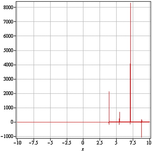
Fig. 2 3D soliton profile of Eq. (4.8)(4.8) $u(\xi )=a_0+2\sqrt{-\mu }\left(\frac{A_1\text{sinh}(\sqrt{-\mu }\xi )+A_2\text{cosh}(\sqrt{-\mu }\xi )}{A_1\text{cosh}(\sqrt{-\mu }\xi )+A_2\text{sinh}(\sqrt{-\mu }\xi )}\right)\text{,}$(4.8) for different values of α.

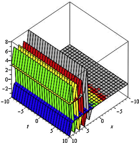
Fig. 3 2D soliton profile of Eq. (4.16)(4.16) $u(\xi )=a_0+\sqrt{\mu }\left(\frac{A_1\text{cos}(\sqrt{\mu }\xi )-A_2\text{sin}(\sqrt{\mu }\xi )}{A_1\text{sin}(\sqrt{\mu }\xi )+A_2\text{cos}(\sqrt{\mu }\xi )}\right)-\sqrt{\mu }{\left[\frac{A_1\text{cos}(\sqrt{\mu }\xi )-A_2\text{sin}(\sqrt{\mu }\xi )}{A_1\text{sin}(\sqrt{\mu }\xi )+A_2\text{cos}(\sqrt{\mu }\xi )}\right]}^{-1}+b_1\sqrt{\sigma \left(1+\frac{{(A_1\text{cos}(\sqrt{\mu }\xi )-A_2\text{sin}(\sqrt{\mu }\xi ))}^2}{{(A_1\text{sin}(\sqrt{\mu }\xi )+A_2\text{cos}(\sqrt{\mu }\xi ))}^2}\right)}+\frac{\sigma b_1}{\sqrt{\sigma \left(1+\frac{{(A_1\text{cos}(\sqrt{\mu }\xi )-A_2\text{sin}(\sqrt{\mu }\xi ))}^2}{{(A_1\text{sin}(\sqrt{\mu }\xi )+A_2\text{cos}(\sqrt{\mu }\xi ))}^2}\right)}}$(4.16) for different values of α.

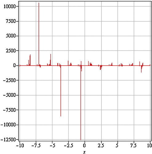
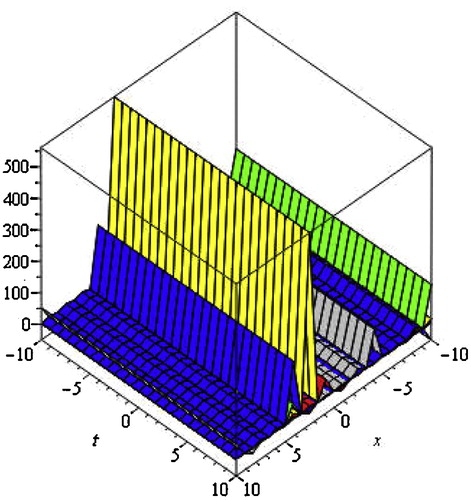
Fig. 4 3D soliton profile of Eq. (4.16)(4.16) $u(\xi )=a_0+\sqrt{\mu }\left(\frac{A_1\text{cos}(\sqrt{\mu }\xi )-A_2\text{sin}(\sqrt{\mu }\xi )}{A_1\text{sin}(\sqrt{\mu }\xi )+A_2\text{cos}(\sqrt{\mu }\xi )}\right)-\sqrt{\mu }{\left[\frac{A_1\text{cos}(\sqrt{\mu }\xi )-A_2\text{sin}(\sqrt{\mu }\xi )}{A_1\text{sin}(\sqrt{\mu }\xi )+A_2\text{cos}(\sqrt{\mu }\xi )}\right]}^{-1}+b_1\sqrt{\sigma \left(1+\frac{{(A_1\text{cos}(\sqrt{\mu }\xi )-A_2\text{sin}(\sqrt{\mu }\xi ))}^2}{{(A_1\text{sin}(\sqrt{\mu }\xi )+A_2\text{cos}(\sqrt{\mu }\xi ))}^2}\right)}+\frac{\sigma b_1}{\sqrt{\sigma \left(1+\frac{{(A_1\text{cos}(\sqrt{\mu }\xi )-A_2\text{sin}(\sqrt{\mu }\xi ))}^2}{{(A_1\text{sin}(\sqrt{\mu }\xi )+A_2\text{cos}(\sqrt{\mu }\xi ))}^2}\right)}}$(4.16) for different values of α.

6 Conclusions

In this paper, we applied the extended $\left(\frac{G^{\prime }}{G}\right)\text{-expansion}$ method for the nonlinear Calogero–Bogoyavlinskii–Schiff equation of fractional order. By using this method, some new traveling wave solutions of this equation are successfully obtained. These solutions include hyperbolic function solutions and trigonometric function solutions. When the parameters are taken as special values, new solitary wave solutions, periodic solutions are given. The resultshow that the extended $\left(\frac{G^{\prime }}{G}\right)\text{-expansion}$ method is direct, effective and can be applied to many other nonlinear fractional PDEs in mathematical physics.

Notes

Peer review under responsibility of Taibah University.