A combined approach of geostatistics and geographical clustering for delineating homogeneous zones in a durum wheat field in organic farming

Abstract

Agricultural practices need to be adapted to variable field conditions to increase farmers’ profitability and environmental protection, so contributing to sustainability of farm management. This study proposes a combined approach of multivariate geostatistics and non-parametric clustering to delineate homogeneous zones that could be potentially managed with the same strategy. In a durum wheat field of Southern Italy, in organic farming, some soil physical and chemical properties (electrical conductivity; pH; exchangeable bases; total nitrogen; total organic carbon; available phosphorous), elevation and the Normalized Difference Vegetation Index were determined and interpolated by using geostatistics.

The clustering approach, applied to the (co)kriged estimates of the variables, produced the delineation of four sub-field zones. A significant relation between soil fertility and yield was not found in such zones. Despite this, the proposed approach has the potential to be used in future applications of precision agriculture. Further work could focus on site-specific nitrogen fertilization with suited machinery.

Keywords:

• Multivariate geostatistical approach
• Non-parametric clustering
• Homogeneous zones
• Precision fertilization
• Organic agriculture

Abbreviations:

• PA
• Precision Agriculture
• EC_a
• Electrical Conductivity
• VI_s
• Vegetation Indices
• NDVI
• Normalized Difference Vegetation Index
• NIR
• Near-Infrared
• EMI
• Electromagnetic Induction
• EC_aV
• Electrical Conductivity in Vertical mode
• EC_aH
• Electrical Conductivity in Horizontal mode
• DGPS
• Differential Global Positioning System
• LMC
• Linear Model of Coregionalization
• k
• ordinary kriging
• lk
• linear kriging
• KED
• Kriging with External Drift
• ck
• co-kriging

1 Introduction

In traditional farm management, fertilization rate does not vary within a single field. Therefore, the excessive use of agro-chemicals in some parts of the field can degrade soil, pollute water bodies and contaminate the atmosphere, as it was tested in some semi-arid Mediterranean areas [1], whereas in other parts the insufficient fertilizer use can decrease crop production.

Precision Agriculture (PA) aims to optimize farming management also by applying fertilizers how much, where and when they are needed, to avoid under- and over-applications. The spatial and temporal variability of soil and crop characteristics can then be turned into a spatially variable application of agro-resources [2].

The site-specific use of fertilizers is expected not only to increase productivity, but also to reduce environmental impact and costs of fertilization. This approach could enable farmers to manage nutrient applications more efficiently [3]. Therefore, PA technologies can contribute to sustainability of agriculture [4]. Although the potential of PA technologies in organic farming systems has not been widely studied, they might be matched with the more basic agro-ecological principles of organic agriculture (e.g. reduced environmental impact and energy use).

The spatial and temporal variability in soil properties and meteorological conditions may affect crop growth, yield and yield quality parameters, even in the same growing season. It then becomes very critical assessing field variability with precision, to produce ‘prescription maps’. These maps are produced with the aim of developing spatially variable-rate fertilizer recommendations [5].

Coupling the information from on-the-go apparent soil electrical conductivity (EC_a) sensors with crop sensors has been showing to be effective in delineating areas of different yield response [6]. Soil electrical conductivity is usually related to a range of physical and chemical properties, across different field areas, and can effectively supplement sparse soil information [7,8]. So, EC_a can be used to improve the estimation of soil variables when they are spatially correlated among them.

Remote and/or proximal sensing of crop vegetation can be excellent high-density data sources to assess plant growth, from a georeferenced location to another one, within and between crop seasons. Multi-spectral reflectance data can be converted into vegetation indices (VI_s), to estimate or represent crop growth. They are commonly obtained by using linear combination or ratios of red, green and near-infrared spectral bands [9]. The most widely known vegetation index is the Normalized Difference Vegetation Index (NDVI), which can be used to estimate plant vigour or green biomass. The NDVI is calculated basing on the fact that photosynthetically active vegetation strongly absorbs the incident radiation in the visible red wavelengths (centred in 670 nm), and reflects in the near-infrared wavelengths (NIR; centred in 780 nm) [10].

Adequate techniques of data analysis are then necessary to detect and model the fine-scale spatial relationship among the study variables of different types, and to identify the main factors controlling within-field variability.

After crop and soil data collection, the next step consists of using interpolation techniques to create maps of soil characteristics. Several studies on PA have been focused on the combination of different layers of information (i.e. several kinds of soil data and multi-temporal crop data) to delineate management zones [11–13[11] [12] [13]]. This delineation has been considered as a practical and cost-effective approach to site-specific management of soil fertility. The management zones are defined as subfield regions, within which the effects on the crop of different factors (i.e., seasonal differences in weather, soil, agricultural practices, etc.) are expected to be more or less uniform. The field should be divided into few relatively uniform MZ_s, considering that numerous small irregularly shaped zones are more difficult to manage [14,15].

Cluster analysis procedures have been effectively used to divide a field into sub-areas that could be uniformly managed [16]. Similar individuals are grouped into distinct classes or ‘clusters’ based on the properties measured for each individual [11]. Most traditional clustering techniques aim to gain insight into the inherent structure of the data and produce natural groups in the attribute space, without any reference to geographical position. This kind of approach does not account for any spatial correlation between observations. Also, it takes little account of gradual change either from one class to another or within any one class. The reason is because it is assumed that the variation of most properties is less within clusters than between clusters. To ensure spatial contiguity because of spatially continuous variation of soil and crop, a clustering algorithm that applies spatial constraint is required. Methods based on estimation of non-parametric probability density function have proven to be the ones with the least bias [17]. According to this approach, clusters are defined as regions surrounding a local maximum of probability density function or a set of local maxima that are strongly correlated. An advantage is that, giving a large enough sample, clusters of unequal size and variance with highly irregular shapes can be detected.

Increasing amount of references about site-specific treatments in winter wheat can be found [18,19]. The objective of this research was to propose a preliminary combined approach of geostatistics and non-parametric clustering. The aim was to merge different data in order to produce a partition of the field into a set of homogeneous zones of manageable size, in a durum wheat field in organic farming. The approach here used is flexible enough to be extended to any number of variables and can combine all data to provide a partition into a number of compact clusters.

2 Materials and methods

2.1 Study site and field trial

The study was carried out during the growing season 2009-2010 at the CRA-Cereal Research Centre, located in Foggia (Southern Italy, 41° 27′ 36.720″ N, 15° 30′ 03.494″ E; 90 m above sea level), on a 3-ha field cropped with rainfed durum wheat (Triticum durum Desf. cv Claudio), under organic farming management.

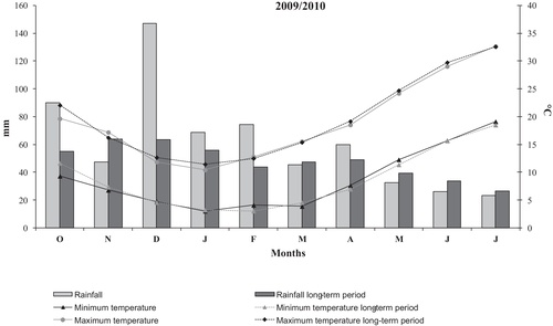
The soil is of alluvial origin, classified as Typic Calcixerept [20] and the climate is Mediterranean, characterized by a dry season between May and September and a cold season from October-November to March-April [21].

In Figure 1 the monthly mean temperatures and the rainfall in the wheat cropping season, recorded at the agro-meteorological station of the Centre, were compared with the long-term averages (1951-2007). The rainfall during November to July period was higher by 10% than the long-term average that was 478 mm. Moreover, the highest rainfall was observed in December (147 mm), thus leading to postpone the sowing to the mid January 2010.

Figure 1 Monthly averages maximum and minimum temperatures (solid line) and rainfall (bars) for the study site, compared to the long-term period 1951-2007.

According to the local practices, a uniform fertilization rate of about 80 kg N ha⁻¹ was used. This rate was split-applied with 1/3 of fertilizer applied, before sowing, as organo-mineral fertilizer (FERBAL SOL 5-14, Ferbal Materias Primas, S.L.), and 2/3 top-dressed at the end of tillering stage (BBCH scale = 29; [22]) as commercial organic fertilizer (FERTIL12.5, ILSA S.p.A.). Both fertilizers are allowed in organic farming.

2.2 Soil sampling and analyses

At the beginning (November 2009) of the field trial, soil samples were taken up to 0.30 m depth in 50 georeferenced locations, at an average distance of 22 m. The locations of the samples were chosen so that they evenly covered the field, by using a k-means algorithm which treats each sample as the centroid of an individual cluster [23]. The number of samples was limited by financial constraints but was sufficient for variogram estimation according to Webster and Oliver [24], who recommended collection of at least 50 sampling points.

The soil samples were air dried, ground to pass through a 2-mm sieve and then analyzed. The following soil characteristics were determined: total organic carbon (TOC; g kg⁻¹), by using the Walkley–Black method [25]; pH measured in a 1:2.5 (w/v) soil/water mixture, using a combination electrode; total nitrogen (N; g kg⁻¹) content, by the Kjeldahl method; available phosphorus (P; mg kg⁻¹), by using the ammonium molybdate-ascorbic acid method, according to Olsen and Sommers [26]; exchangeable bases (K, Ca, Na and Mg; mg kg⁻¹) extracted by BaCl₂ and N(CH₂OHCH₂)₃, according to Page et al. [26] methodologies, and assayed by Inductively Coupled Plasma-Optical Emission spectrometry ICP-OES.

2.3 EMI and DGPS elevation surveys

An electromagnetic induction (EMI sensor) survey was performed on March 3rd 2010. The field was surveyed with an average air temperature of 8 °C and soil water conditions close to field capacity. The survey was performed when about 44% of the seasonal rainfall had already occurred (Figure 1).

The used ground conductivity meter (EM38DD, Geonics, Ltd, Ontario-Canada) allowed to measure EC_a (mS m⁻¹) simultaneously in two orientations, with a different depth response profile: i) in vertical mode (EC_aV) with maximum sensitivity at approximately 0.40-m soil depth, and ii) in horizontal mode (EC_aH) with maximum sensitivity at the soil surface.

The sensor was carried across the field using a tractor, along 15 transects parallel to the longer axis of the field and approximately spaced 7 m apart. Moreover, the sensor was calibrated and nulled according to the manufacturer instruction, before starting the measurements.

Locations and elevation (m) were recorded using a Differential Global Positioning System (DGPS; HiPer® Pro, TOPCON) with centimetre accuracy, both horizontal and vertical. The signal was corrected in Real Time Kinematic (RTK) GPS. The DGPS was attached to EM38DD and both types of data were simultaneously recorded each one second (about 2-3 meters apart).

2.4 Crop spectral measurements

An 8-channel handheld sensor (SKL-908, model SpectroSense2+, SKYE Instruments, UK) was used to measure the reflected electromagnetic radiation from the canopy at the 50 georeferecend locations.

The data were collected on two dates, 03/15/2010 and 04/27/2010 (from now on indicated as: 03/15 and 04/27), corresponding to tillering (BBCH scale = 23) and the stem elongation (BBCH scale = 37) stages of growth, respectively [22].

Measurements were performed putting the sensor arm at a height of 1.5 m above the canopy (area of measurement of 0.35 m²), under clear sky conditions, within 2 h of solar noon. The NDVI ratio was obtained from a pair of identical 2 channel sensors: one measuring the incident radiance at Red (670 nm) and NIR (780 nm) wavelengths, while the second simultaneously measuring radiation at Red and NIR reflected upwards, so to eliminate fluctuations in solar radiation. The index was then determined in terms of reflection.

2.5 Yield monitoring

Yield data were recorded by a John Deere combine equipped with a yield monitor system. The spatial resolution (yield unit size) was of 6 m by 2 m, with the shorter side along the moving direction. After recording, yield data were normalized to 13% grain moisture. On the basis of yield commonly obtained in the study area, values less than 1.6 and greater than 7 t ha⁻¹ were removed. The resulting data were interpolated by kriging and mapped, as it was previously reported in Diacono et al. [27]. A box plot was then drawn to compare the yield of the clusters which were determined in this study.

2.6 Statistical and Geostatistical techniques

2.6.1 MultiGaussian approach

Even if ordinary cokriging does not require a normal distribution of data, variogram modelling is sensitive to strong departures from normality, because a few exceptionally large outliers may contribute to very large squared differences [28].

To avoid this problem, multiGaussian approach was used to produce the maps of the variables. Such approach consists of different steps, starting with transformation of the initial attributes into Gaussian-shaped variables with zero mean and unit variance. This procedure, known as ‘Gaussian anamorphosis’, consists of determining a mathematical function to transform a variable with a standardized Gaussian distribution into a new variable with any distribution [28]. This transformation is made by using an expansion of Hermite polynomials [28] restricted to a finite number (30-100) of terms.

Preliminary to interpolation of a set of variables which are correlated among them, there is modelling the coregionalization using the so-called Linear Model of Coregionalization (LMC), developed by Journel and Huijbregts [29]. LMC considers all the studied variables as the result of the same independent physical processes, acting at N_s spatial scales. The simple and cross variograms of the variables are all modelled by linear combinations of the same N_s variograms standardized to unit sill [5]. Fitting of LMC to the experimental variograms of the Gaussian transformed variables is performed by weighted least-squares approximation (method of moments). This is done under the constraint of positive semi-definiteness of the coregionalization matrix (the matrix of the estimated sills) corresponding to each spatial scale, through an iterative procedure [30].

Otherwise, a univariate approach, consisting in variogram fitting and kriging procedures, must be applied for those variables that are not significantly correlated with the others in a data set.

Finally, the estimated gaussian variables are submitted to back transformation, through the mathematical model calculated in the Gaussian Anamorphosis, and the raw variable estimates are mapped.

2.6.2 Interpolation procedures

The individual Gaussian variables were interpolated using different approaches: ordinary kriging (k); linear kriging (lk); Kriging with External Drift (KED) and multi-collocated co-kriging (ck).

Simple and ordinary kriging are the most basic kriging methods, which use only primary information and also provide an error variance [31]; linear kriging is an approach of simple kriging requiring the estimation of a linear function of spatial covariance.

The interpolation technique of KED is a method of non-stationary geostatistics [32]. The basic hypothesis of KED is that the non constant expectation of the variable (known only at a small set of points in the study area) can be written as the sum of a basis of polynomials of the coordinates and a linear combination of secondary variables, exhaustively known at each node of a grid in the same area (external drift) [33]. The spatially correlated random part is instead expressed by a generalized covariance function of the separation distance.

Multi-collocated co-kriging, as described by Castrignanò et al. [34], is a way of integrating secondary information (auxiliary variable), exhaustively known, in primary variable modelling. For estimation, the method uses the auxiliary variable at the grid node and at the points in which also the primary variable is available within the interpolation neighbourhood. There is actually little loss of information, compared to full cokriging, because the co-located secondary datum tends to screen the influence of more distant secondary data. Therefore, incorporating dense secondary information can really lead to more consistent description of the property under study. Moreover, it produces more accurate estimates of the primary variables.

In our study, the dataset was processed in the following way: i) a LMC was fitted on the raw EC_a data in the two polarization modes, and co-kriging was used to produce estimates at the nodes of a 1 m x 1m-cell grid; ii) DGPS elevation data was non-stationary, so the drift and the generalized covariance were calculated. KED was then applied to produce the estimates at the nodes of the previous grid; iii) to perform a joint multivariate analysis on soil chemical properties and geophysical variables, the estimates of EMI and elevation were migrated to the locations of the nearest soil samples. The global dataset was then split into two subgroups on the basis of the spatial correlation: a) the first subset, including NDVI (on 04/27), pH, TOC and K, for which a univariate approach was preferred, because of non significant correlation (P < 0.05) among the variables. More specifically, ordinary kriging was used to interpolate NDVI and pH, and linear kriging for TOC and K; b) the second subset, including P; Na; N; Mg; Ca and NDVI on 03/15; EC_aH, EC_aV and elevation estimates. A multivariate approach was used because of the significant (P < 0.05) correlation among most variables. A LMC was fitted and multi-collocated co-kriging was applied, choosing EC_aH as (auxiliary) collocated variable. The choice was made because EC_aH was the most correlated variable with the soil variables and seemed to be more sensitive to the farm management (i.e. soil tillage). The data were estimated at the nodes of the same previous grid.

Geostatistical procedures were applied by using the software package ISATIS®, release 11.2 [35].

2.6.3 Clustering approach

According to Scott [36], an algorithm based on non-parametric estimate of probability density function was used to divide the fields into a number of soil clusters or classes, so summarizing the complex multivariate variation of the field in a restricted number of homogeneous zones. This approach uses hyperspherical uniform kernels of fixed radius to estimate density. The density at any point of the attribute hyperspace is computed by dividing the number of observations, within a sphere centred at the point, by the product between the total number of observations and the volume of the sphere. The size of the sphere is determined by a pre-specified smoothing parameter (R), which represents the kernel radius and is expressed as a Euclidean distance. The algorithm searches the local mode of the density function through an iterative approach. There is no simple answer to the question of which smoothing parameter to use, even if the problem of choosing how much must be smoothed is of crucial importance in density estimation. However, we agree with Silverman [37] that the appropriate choice of smoothing parameter must always be influenced by the purpose for which the density estimate is to be used. In our study density estimation is used to explore the data and suggest a partition of the field into a reasonable number of practical management zones. Therefore, we have preferred to choose the smoothing parameter subjectively, by trying several different values, rather than to use some automatic or statistical method, even if more objective [17]. The number of clusters is a function of the smoothing parameters and generally tends to decrease as the smoothing parameter increases. However, the relationship is not strictly monotonic and several different values of the smoothing parameter have generally to be specified before seeing as the number of cluster varies. The clustering method is not inherently hierarchical. However, it calculates the probability that, in repeated sampling, the estimate of the number of clusters exceeds the true number of them and then allows performing statistical tests of significance [38].

As the variables were not measured in comparable units, they were scaled to zero mean and unit variance to have equal weight in the analysis.

The geostatistical estimates of all studied variables and the spatial co-ordinates were included in the clustering algorithm. Unsupervised classification identifies statistically similar clusters without taking into account proximal information. As a consequence, the result may contain several relatively small clusters of one zone interspersed among others. To reduce this effect, interpolated data were used instead of sample data for clustering, to obtain more homogeneous and manageable zones, and the coordinates were included in the attribute space [17]. The clustering approach was implemented with the MODECLUS procedure of SAS/STAT software package [39].

3 Results and discussion

The descriptive statistics of all soil properties and measurements are summarized in Table 1. The data configuration was isotopic [28], i.e., all the variables were measured at each location. A general moderate variability within the field, as it results from CV values (<0.5), can be detected. Elevation, NDVI on 04/27 and pH showed departures from the gaussian distribution (the hypothesis of normality was refused on the basis of χ² test, at the 5% level of probability), so they were transformed into Gaussian scores.

Table 1 Descriptive statistics of soil properties and NDVI measurements.

Variable	Min	Max	Mean	Median	SD	CV	Skewness	Kurtosis
pH	7.01	7.28	7.10	7.10	0.04	0.01	1.18	6.92
Ca (mg kg^−1)	5050.55	6168.13	5623.98	5625.35	264.42	0.05	0.16	2.30
K (mg kg^−1)	1210.28	2270.56	1437.89	1387.06	180.57	0.13	2.24	10.06
Mg (mg kg^−1)	184.64	348.27	244.49	240.97	31.45	0.13	0.84	4.22
Na (mg kg^−1)	62.26	142.72	92.92	93.91	18.73	0.20	0.42	3.17
P Olsen (mg kg^−1)	13.60	37.40	23.66	23.10	5.27	0.22	0.69	3.22
N (g kg^−1)	0.58	1.15	0.98	1.00	0.12	0.13	-1.29	4.75
TOC^a (g kg^−1)	9.64	13.13	11.08	11.06	0.73	0.07	0.18	2.98
ECaH^b (mS m^−1)	34.38	86.25	59.71	60.13	9.02	0.15	-0.26	2.66
ECaV^c (mS m^−1)	23.13	69.75	46.10	46.75	7.85	0.17	-0.22	3.22
Elev.^d (m)	89.44	92.14	90.79	90.82	0.71	0.01	0.02	1.69
NDVI^e 03/15	0.22	0.44	0.37	0.38	0.05	0.15	-1.25	3.87
NDVI 04/27	0.67	0.89	0.81	0.82	0.05	0.06	-0.64	2.78

Note: ^a = total organic carbon; ^b = apparent soil electrical conductivity in horizontal mode; ^c = apparent soil electrical conductivity in vertical mode; ^d = elevation recorded using a Differential Global Positioning System; ^e = Normalized Difference Vegetation Index.

3.1 EMI and DGPS elevation results

The isotropic LMC model, which was fitted to the experimental variograms of the EMI variables, included the following basic structures: i) a nugget effect; ii) a spherical model with a range of 30 m and iii) a spherical model with a range of 80 m.

The spatial maps of the estimated EMI data in the two polarization modes, are shown in Figure 2 (a-b). The EC_aH patterns looked parallel to the wheat rows and the tillage drills, showing the highest values in the western part of the field (Figure 2a). The EC_aV map (Figure 2b) showed a different pattern distribution, with higher values localized in the north area and in some sparse spots in the rest of the field.

Figure 2 Spatial maps of (a) electrical conductivity in horizontal mode (EC_aH); (b) electrical conductivity (mS m⁻¹) in vertical mode (EC_aV) and (c) elevation (Color scale uses isofrequency classes). The coordinate system was Universal Transverse Mercator (UTM- Zone 33 N) and the datum (reference ellipsoid) was WGS84.

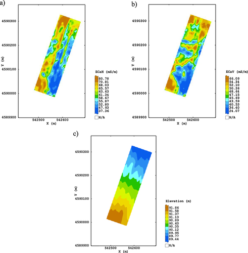
As the DGPS elevation variogram looked unbounded, the estimated drift included an intercept and a linear function in the spatial coordinates X and Y but no external variables. The generalized covariance was modelled with a spline structure of the third order with scale of 44 m and sill equal to 0.096. In the map of elevation (Figure 2c) the systematic linear component of variation prevailed on the stochastic one, and a clear decreasing trend from SW to NE can be observed.

3.2 NDVI (on 04/27), pH, TOC and K results

The models, fitted to the experimental variograms of the Gaussian transformed NDVI and pH, included the following structures: i) a nugget effect and a spherical model with range of 95.5 m, for NDVI; ii) a nugget effect and a spherical model with range 65.9 m, for pH.

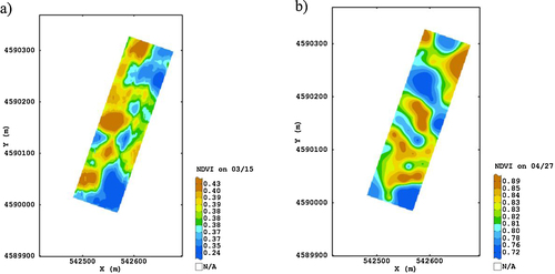
The map of the estimated NDVI on 04/27 showed a quite erratic spatial pattern with higher values particularly in the central-southern part of the field (Figure 3b), whereas the pH map showed higher values in a north-eastern area (Figure 4a).

Figure 3 Spatial maps of Normalized Difference Vegetation Index (NDVI) at two growth stages: (a) at 03/15 and (b) at 04/27 of 2010 (Color scale uses isofrequency classes). The coordinate system was Universal Transverse Mercator (UTM - Zone 33 N) and the datum (reference ellipsoid) was WGS84.

Figure 4 Spatial maps of soil properties: pH; K (mg kg⁻¹); TOC (g kg⁻¹); N (g kg⁻¹); P (mg kg⁻¹); Mg (mg kg⁻¹); Ca (mg kg⁻¹) and Na (mg kg⁻¹) (Color scale uses isofrequency classes). The coordinate system was Universal Transverse Mercator (UTM- Zone 33 N) and the datum (reference ellipsoid) was WGS84.

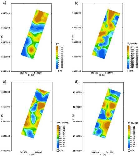
As regards the map of K, higher values occurred at the northern and central-western boundaries (Figure 4b). The highest TOC occurred along the western and eastern borders of the field (Figure 4c).

3.3 Multivariate approach for correlated variables (P, Na, N, Mg, Ca and NDVI on 03/15; ECaH, ECaV and elevation estimates)

The fitted isotropic LMC included the following basic structures: i) a nugget effect; ii) a cubic model with range of 60 m and iii) a K-Bessel model with scale 140 m and the parameter equal to 1.

The estimates maps of the raw variables showed some distinct spatial patterns and also some degree of spatial association among the different soil and plant attributes.

The map of NDVI on 03/15 showed higher values along the western boundaries (Figures 3a) and the estimated values corresponded on average to green and healthy vegetation at the growing stage surveyed.

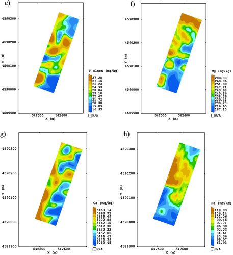
In regard to the soil macro-nutrients, the highest N contents were located in the middle and south-eastern parts of the field (Figure 4d). Similarly, the map of P Olsen content showed a structure characterized by higher values in the central zone, but also in the south-western parts of the field (Figure 4e).

Though the two depicted NDVI maps were related to the green biomass of wheat, they did not reveal a clear relationship with total soil N. This result confirmed as crop growth depends on many correlated factors acting in the soil, besides such macro-nutrient availability [40].

It was observed [27] that the northern part of the field and partly the central one were finer textured. Moreover, April was more rainy compared to March by 33% (Figure 1) and the crop was in a stage of increased nutrient uptake. Both texture and rainfall could be the cause of the different spatial pattern observed between the two NDVI maps. In fact, NDVI on 04/27 more clearly showed an influence of the spatial distribution of texture which might be the reason both of reduced N losses by leaching and better N-use efficiency [41].

As the NDVI estimates at the two dates were not correlated between them, temporal response of wheat to the spatial variation in soil properties might depend both on climatic conditions and phenological stage.

The highest Mg contents were localized in the north, corresponding to higher pH values, and in the western parts of the field (Figures 4f).

The Ca values were particularly higher along the western boundaries, approximately reproducing the same partition observed for the EC_aH (Figure 4 g), whereas the Na map looked much better structured with higher values located in the north-central part of the field (Figures 4 h).

The above described distributions of soil properties did not show common spatial macro-structures clearly defined. The quite erratic spatial patterns of most variables might be attributed to various factors, jointly operating at field scale, as previous fertilization, soil texture and moisture content. According to Castrignanò et al. [42], texture may cause different water conditions in the soil, which may affect nutrient availability to crop during the growing season. This is particularly critical for a rainfed crop as the durum wheat in the study site.

3.4 Delineating homogeneous zones

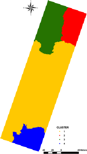
The multivariate heterogeneity of the field was synthesized by clustering. After several trials, the smoothing parameter in the density algorithm was chosen as R= 1.8, because it produced a subdivision of the field into 4 statistically (probability < 0.0001) significant clusters. This partition best accorded with the description of spatial variation in the field, through a visual inspection of the thematic maps previously described.

In Table 2, the means and standard deviations of the soil attributes for each cluster are reported. It can be summarized that cluster 1 was characterized by the greatest level of chemical fertility, due to the highest values of N and TOC; cluster 2 showed the lowest N values; cluster 3 had a medium soil fertility level; whereas cluster 4 showed the lowest P, K and TOC values, so appearing the least fertile cluster.

Table 2 Descriptive statistics of the clusters.

	Cluster 1		Cluster 2		Cluster 3		Cluster 4
Variable	Mean	SD	Mean	SD	Mean	SD	Mean	SD
kpH	7.09	0.01	7.10	0.00	7.10	0.00	7.09	0.00
ckCa	5660.63	249.96	5554.51	173.25	5606.26	160.20	5501.39	200.09
lkK	1427.85	88.94	1427.84	132.49	1533.42	193.60	1311.81	28.59
ckMg	238.84	11.86	258.37	14.84	255.51	14.55	211.41	12.08
ckNa	92.92	12.17	88.96	6.21	100.26	6.21	70.15	5.15
ckP	24.44	2.98	20.33	0.84	23.70	2.06	19.14	1.34
ckN	1.00	0.07	0.96	0.02	0.99	0.03	0.98	0.02
lkTOC	11.27	0.45	10.79	0.52	10.82	0.62	10.74	0.28
ckECaH	58.76	8.20	63.79	3.17	67.13	6.23	54.67	9.45
ckECaV	45.42	6.64	52.30	2.81	49.45	4.38	40.67	8.23
KED^aelevation	90.86	0.49	89.72	0.15	89.93	0.21	91.55	0.14
ckNDVI 03/15	0.38	0.01	0.36	0.01	0.38	0.01	0.33	0.03
kNDVI 04/27	0.82	0.01	0.83	0.00	0.80	0.01	0.80	0.00

Note: ^a= kriging with external drift; ck= cokriging estimated variables; k= kriging estimated variable; lk = linear kriging estimated variables.

Figure 5 shows the box plots (a) for total N and (b) for TOC contents, in each cluster, which were selected as two of the most important parameters determining soil chemical fertility for wheat cultivation. As regards N, although the means were not statistically different, the spatial distribution of cluster 1 was characterized by larger variability, due to its bigger size. The results showed as most residual variation still occurs within each cluster. The total N content was minimum in cluster 2, despite high clay content was observed in this area [27]. This apparent contradiction might be explained as due to an interaction between biotic (i.e. micro-organisms) and/or other abiotic factors (i.e. monthly temperatures).

Figure 5 Box plots of (a) nitrogen (N) and (b) total organic carbon (TOC) contents in each cluster.

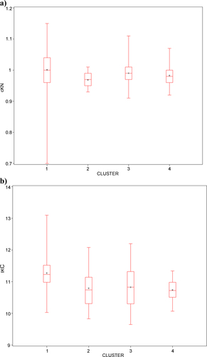
Total organic carbon is another relevant soil factor controlling water-holding capacity [1], particularly for rainfed wheat growing in a dry environment as the study site. Again, the second box plot (Figure 5b) did not show significant differences in the variable among the clusters. However, cluster 1 was characterized by tendentially higher values of TOC and a larger variability.

The map of the clusters shows the partition of the field into 4 sub-field zones (Figure 6): the cluster 1 extending for most part of the field, whereas the other three clusters are restricted at the northern border (clusters 2 and 3) and the south-eastern corner (cluster 4).

Figure 6 Clusters obtained by the non-parametric density algorithm.

Figure 7 shows the box plot of the yield in each of these zones. It doesn’t reveal any significative difference among the clusters, even if the cluster 4 was basically the least productive, confirming its lowest overall fertility. Moreover, in the yield map reported in Diacono et al. [27] the extremely erratic variation of production did not reflect the above delineation in clusters.

Figure 7 Box plot of the yield level in each cluster.

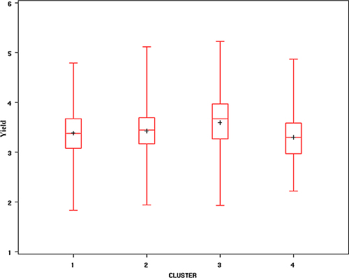
Therefore, the spatial heterogeneity of soil chemical properties did not seem to have a significant impact on wheat production during the trial period. This outcome needs to be verified over more cropping seasons.

3.5 Fertilization recommendations

The crop N demand depends on the available N in soil during the growth period, which is particularly related to soil organic matter and fertilizer supply [40]. A plan of wheat fertilization should take into account crop N needs and N credit deriving from mineralized organic matter.

As a matter of fact, differences in soil fertility were not statistically significant among clusters and their productive level was comparable, owing to the large residual variation within each homogeneous zone. The study field should be fertilized with spatially variable rates of N. In particular, the borders of the clusters could be rectified by drawing 10 m (according to working width of a common fertilizer spreader) x 330 m strips parallel to the longer side of the field, in order to facilitate the work of the fertilizer spreader.

According to our above-mentioned study [27], organic carbon mineralization rate was consistent during the cropping season in this site, but differed spatially. The northern, middle and southern areas were characterized by relatively lower carbon mineralization rates compared to western and eastern spots in the field. This outcome might suggest the need for a higher organic-mineral fertilizer application in the sub-field zones that corresponded to the areas of lower carbon mineralization rates (i.e. lower N credit for the crop).

4 Conclusions

Research in precision agriculture has focused on dividing a field into few relatively uniform homogeneous zones as a practical, environmentally sustainable and cost-effective approach for managing soil variability. Such an approach can be well matched with organic agriculture principles.

In our study, soil characteristics and Normalized Difference Vegetation Index were used to delineate homogeneous zones in a durum wheat field, by adopting multivariate geostatistics combined with a non parametric density algorithm. Given the complexity of the interactions among the factors that affect crop growth, a multivariate approach to the determination of such zones was advisable.

The research has proved that geostatistical techniques may be used as a powerful tool to assess the spatial variability of the soil. However, contrary to expectations we did not find significant differences in soil fertility and yield among the delineated homogeneous zones, which greatly differed in their size. Site-specific nitrogen fertilization could be adapted to this field with suited machinery. Future work should focus also on using radiometric sensing of N status of vegetation to fulfil crop demand, varying across the field, with timely applications of fertilizer.

Moreover, there is a need for more research on environments like the one above described to study the spatial and temporal variability of yield over many years.

Acknowledgements

The work has been supported by Italian Ministry of Agriculture and Forestry Policies under contract n. 24324/7742/2009 (“Sistemi colturali e interventi agronomici innovativi in agricoltura biologica” BIOINNOVA, Coordinator: Dr. Domenico Ventrella, CRA–SCA, Research Unit for Cropping Systems in Dry Environments, Bari).

References

- M. Diacono F. Montemurro Long-term effects of organic amendments on soil fertility. A review E. Lichtfouse M. Hamelin M. Navarrete P. Debaeke Sustainable agriculture, Springer Science + Business Media B.V 2011 EDP Sciences 761 786
- F.J. Pierce P. Nowak Aspects of precision agriculture Adv. Agron. 67 1999 1 85
- J.L. Boggs DrT.D. Tsegaye T.L. Coleman K.C. Reddy A. Fahsi Relationship between hyperspectral reflectance, soil nitrate-nitrogen, cotton leaf chlorophyll, and cotton yield: a step toward precision agriculture J. Sustainable Agric. 22 2003 5 16
- R. Bongiovanni J. Lowenberg-Deboer Precision Agriculture Sustainability Precis. Agric. 5 2004 359 387
- A. Castrignanò L. Giugliarini R. Risaliti N. Martinelli Study of spatial relationships among some soil physico-chemical properties of a field in central Italy using multivariate geostatistics Geoderma 97 2000 39 60
- J.C. Taylor G.A. Wood R. Earl R.J. Godwin Soil factors and their influence on within-field crop variability, part II: spatial analysis and determination of management zones Biosystems Eng. 84 2003 441 453
- K.A. Sudduth N.R. Kitchen W.J. Wiebold W.D. Batchelor G.A. Bollero D.G. Bullock D.E. Clay H.L. Palm F.J. Pierce R.T. Schuler K.D. Thelen Relating apparent electrical conductivity top soil properties across the North-Central USA Comput. Electron. Agric. 46 2005 263 283
- D. De Benedetto A. Castrignanò D. Sollitto F. Modugno G. Buttafuoco G. lo Papa Integrating geophysical and geostatistical techniques to map the spatial variation of clay, Geoderma 2011 http://doi:10.1016/j.geoderma.2011.05.005
- D. Rodriguez G.J. Fitzgerald R. Belford L.K. Christensen Detection of nitrogen deficiency in wheat from spectral reflectance indices and basic crop eco-physiological concepts Aust. J. Agric. Res. 57 2006 781 789
- S. Biewer S. Erasmi T. Fricke M. Wachendorf Prediction of yield and the contribution of legumes in legume-grass mixtures using field spectrometry Precis. Agric. 10 2009 128 144
- R.M. Lark Forming spatially coherent regions by classification of multivariate data: An example from the analysis of maps of crop yield Int. J. Geog. Inf. Sci. 12 1998 83 98
- E. Vrindts M. Reyniers P. Darius J. De baerdemaeker M. Gilot Y. Sadaoui M. Frankinet B. Hanquet M.-F. Destain Analysis of soil and crop properties for precision agriculture for winter wheat Biosystems Eng. 85 2003 141 152
- J.J. Fridgen N.R. Kitchen K.A. Sudduth S.T. Drummond W.J. Wiebold C.W. Fraisse Management Zone Analyst (MZA): Software for Subfield Management Zone Delineation Agron. J. 96 2004 100 108
- J.A. Taylor A.B. McBratney B.M. Whelan Establishing management classes for broadacre agricultural production Agron. J. 99 2007 1366 1376
- A. Castrignanò, M.T.F. Wong, F. Guastaferro, Delineation of management zone using multivariate geostatistics and EMI data as auxiliary variable, in: Proceedings of the 18th Symposium of the International Scientific Centre of Fertilizers, More Sustainability in Agriculture: New Fertilizers and Fertilization Management, Fertilitas Agrorum (2010) 241-248 (ISSN 1971-0755).
- F. Morari A. Castrignanò C. Pagliarin Application of multivariate geostatistics in delineating management zones within a gravelly vineyard using geo-electrical sensors Comput. Electron. Agric. 68 2009 97 107
- A. Castrignanò G. Buttafuoco M. Pisante N. Lopez Estimating within-field variation using a nonparametric density algorithm Environmetrics 17 2006 465 481
- D. Ehlert J. Schmerler U. Voelker Variable rate nitrogen fertilisation of winter wheat based on a crop density sensor Precis. Agric. 5 2004 263 273
- J.T. Biermacher F.M. Epplin B.W. Brorsen J.B. Solie W.R. Raun Economic feasibility of site-specific optical sensing for managing nitrogen fertilizer for growing wheat Precis. Agric. 10 2009 213 230
- Soil Survey Staff, Soil taxonomy (Second Edition). USDA, National natural resources Conservation Service, Washington D.C., 1999, USA.
- A. Troccoli, S.A., Colecchia, L., Cattivelli, A. Gallo, Caratterizzazione agro-climatica del capoluogo dauno–Analisi della serie storica delle temperature e delle precipitazioni rilevate a Foggia dal 1955 al 2006. Tipografia Digital Print di Cannone s.a.s. (Orta Nova–FG), 2007, pp. 144. (in English: Agro-climatic characterization of Foggia town - Analysis of the historical series of temperature and precipitation, recorded in Foggia from 1955 to 2006. Printed at the Typography Digital Print of Cannone s.a.s.).
- P.D. Lancashire H. Bleiholder P. Langelüddecke R. Stauss T. Van Den Boom E. Weber A. Witzenberger An uniform decimal code for growth stages of crops and weeds Annals of Applied Biology 119 1991 561 601
- J. de Gruijter, D.J., Brus, M.F.P., Bierkens, M. Knotters, Sampling for Natural Resource Monitoring XIV, 332, 2006, p. 91.
- R. Webster M. Oliver Geostatistics for Environmental Scientists. Statistics in practice 2001 Wiley Chichesterp.265
- A. Walkley I.A. Black An examination of the Degtjareff method for determining organic carbon in soils: Effect of variations in digestion conditions and of inorganic soil constituents Soil Sci. 63 1934 251 263
- A.L. Page, R.H., Miller, D.R. Keeny, Methods of Soil Analysis, Part II. 2nd ed., American Society of Agronomy, Madison, Wisconsin, 1982.
- M. Diacono, H. Abd El Rahman, C., Cocozza, D. De Benedetto, A., Troccoli, P., Rubino, A. Castrignanò, Delineation of homogeneous field zones based on soil fertility indices in a durum wheat - chickpea rotation, in: John V. Stafford (Eds.), Precision Agriculture 2011, pp. 164-179, Ampthill, UK.
- H. Wackernagel Multivariate Geostatistics: an introduction with Applications 3rd ed. 2003 Springer Verlag Berlinp388
- A.G. Journel C.J. Huijbregt Mining Geostatistics 1978 Academic Press New York
- C. Lajaunie, J.P. Béhaxétéguy, Elaboration d’un programme d’ajustement semi-automatique d’un modèle de corégionalisation–Theorie, technical report N21/89/G. Paris: ENSMP, 1989, 6 pp.
- P. Goovaerts Geostatistics for natural resources evaluation 1997 Oxford University Press New York
- G. Hudson H. Wackernagel Mapping temperature using kriging with external drift: theory and an example from Scotland Int. J. Climatol. 14 1994 77 91
- B. Cafarelli A. Castrignanò The use of geoadditive models to estimate the spatial distribution of grain weight in an agronomic field: a comparison with kriging with external drifty Environmetrics 22 2011 769 780
- A. Castrignanò G. Buttafuoco R. Comolli A. Castrignanò Using digital elevation model to improve soil pH prediction in an Alpine doline Pedosphere 21 2011 259 270
- Geovariances, Isatis Technical Ref., 11.02 Geovariances and Ecole Des Mines De Paris: Avon Cedex, 2011, France.
- D.W. Scott Multivariate density estimation: theory, practice, and visualization 1992 John Wiley & Sons Inc New York
- B.W. Silverman Density Estimation 1986 Chapman and Hall, CRC New York
- F. Guastaferro A. Castrignanò D. De Benedetto D. Sollitto A. Troccoli B. Cafarelli A comparison of different algorithms for the delineation of management zones Precis. Agric. 11 2010 600 620
- SAS Institute Inc. SAS/STAT Software Release 9.2, Cary, NC, 2010, USA.
- J.K. Ladha H. Pathak T.J. Krupnik J. Six C. van Kesse Efficiency of fertilizer nitrogen in cereal production: retrospects and prospects Adv. Agron. 87 2005 85 156
- M.J.D. Hack-ten Broeke W.J.M. De Groot Evaluation of nitrate leaching risk at site and farm level Nutr. Cycling Agroecosyst. 50 1998 271 276
- A. Castrignanò, B. Basso, M., Pisante, G., Buttafuoco, A., Troccoli, G., Cucci, C. Fiorentino, Delineating management zones using crop and soil variables with a multivariate geostatistic approach, in: Proceedings of the 9th International Conference On Precision Agriculture, [CD-ROM], 2008, Denver (USA).