Execution of novel explicit RKARMS(4,4) technique in determining initial configurations of extra-solar protoplanets formed by disk instability

Peer review under responsibility of National Research Institute of Astronomy and Geophysics.

Abstract

Implementation of a novel embedded Runge–Kutta fourth order four stage arithmetic root mean square technique to determine initial configurations of extra-solar protoplanets formed by gravitational instability is the main goal of this present paper. A general mathematical framework for the introduced numerical technique is described in addition to error estimation description. It is noticed that the numerical outputs through the employed novel RKARMS(4,4) method are found to be more effective and efficient in comparison with the results obtained by the classical Runge–Kutta technique.

Keywords:

• Novel RKARMS(4,4) technique
• Error estimates
• Conductive-radiative
• Disk instability
• Protoplanet

1 Introduction

From literature review it is noticed that the ever-increasing advances in high performance computer technology have enabled several researchers towards science and engineering to employ novel numerical techniques to simulate physical phenomena. Intensive techniques are frequently required for the solution of real time practical problems and they often need the systematic application of a range of elementary techniques. In the development of new numerical methods, simplifications required to be made to progress towards an optimal solution. As a result, numerical algorithms do not usually give the exact answer to a given problem, or they can only tend towards a solution getting closer and closer with each iteration. Numerical techniques exhibit certain computational characteristics during their real time implementation. It is significant to consider these characteristics while selecting a specific technique for implementation. The characteristics which are critical to the success of implementation are accuracy, rate of convergence, numerical stability and efficiency. Numerical algorithms must review the factors such as, determination of the correctness of various steps, reduction of the number of steps, if necessary, and increase in the speed of solving the problem, respectively.

To solve many different problems under signal processing, communication, electronic and transistor circuits, Runge–Kutta (RK) method is being applied to obtain the required solution (Alexander and Coyle, 1990). Shampine and Gordon (1975) discussed the normal order of a RK algorithm having the approximate number of leading terms of an infinite Taylor series, which calculates the trajectory of a moving point. Yaakub and Evans (1993) presented a new fourth order RK method based on the root mean formula for solving initial value problems (IVPs) in numerical studies. A new embedded fourth order RK method which is actually two different RK methods but of the same order p = 4 has been introduced by Evans and Yaakub (1995). Bader (1987, 1998) introduced the RK–Butcher algorithm for finding the truncation error estimates, intrinsic accuracies and the early detection of stiffness in coupled differential equations arising in theoretical chemistry problems. Yaakub and Evans (1999) introduced a new fourth order RK technique for IVPs with error control. Butcher (1987, 1990, 2003) derived the best RK pair along with an error estimates and by all statistical measures it appeared as RK–Butcher algorithms. In order to overcome step-size constraint imposed by numerical stability, many new techniques have been developed in recent past. To confirm this, recently Ponalagusamy and Senthilkumar (2009) proposed a novel fourth order embedded RKARMS(4,4) technique based on RK arithmetic mean and root mean square with error control in detail to solve the real time application problems efficiently in image processing under CNN model. A detailed illustration related to the local truncation error (LTE), the global truncation error (GTE), error estimates and control for fourth order and four stage RK numerical algorithms is eventually addressed by Senthilkumar (2009).

The formation of planetary systems has been a topic of interest to the mankind ever since the dawn of civilization. However, scientific theories for the formation of the system largely date from Descartes (1644) when he proposed his vortex theory in this regard. Since that time many theories have been advanced. In most cases these theories were primarily speculative because of the lack of observational characteristics of the system. Fortunately, for the theorists of today, there are some convenient observational constrains of the system. The two end mechanisms, namely core accretion and disk instability, in principle, can form gas giant protoplanets. Though the core accretion mechanism has been, so far, adopted as the main theory of planetary formation both in our solar system and elsewhere, it fails to explain properly the recently discovered extrasolar protoplanets by direct imaging (see Dodson-Robinson et al., 2009). With this difficulty encountered by the core accretion models, the disk instability model, once in vague, has been reformulated with fragmentation from massive protoplanetary disks and has been advanced through the investigations of many authors (e.g., Boss, 1997; Mayer et al., 2002, 2004; Boley et al., 2010; Cha and Nayakshin, 2011). But this model is also criticized by some investigations with the argument that disk instabilities are unable to lead to the formation of self-gravitating dense clumps (Pickett et al., 2000; Cai et al., 2006; Boley et al., 2007). Although some questions arise as to whether stable protoplanets could be formed or not by disk instability, the idea is believed to be a promising route to the rapid formation of giant planets in our solar system and elsewhere (Boss, 2007). Unfortunately, the initial structures of the protoplanets formed via gravitational instability are still unknown and different numerical models can be found to report different configurations (Helled and Schubert, 2008; Helled and Bodenheimer, 2011).

It is pertinent to point out here that depending upon opacities of grains, present in protoplanets, as well as on initial conditions different investigators assumed different heat transports at different regions of protoplanets at different stages of their evolution. DeCampli and Cameron (1979), in their investigation, assumed initial protoplanets to be fully convective with a thin outer radiative zone as a consequence of higher opacity and much work has since then been devoted to the evolution of planetary system including our own from such types of initial protoplanets (e.g., Bodenheimer et al., 1980; Wuchterl et al., 2000; Helled et al., 2008; Helled and Bodenheimer, 2011). It is well-known that depending on obeying the law $L/4\pi R^2={(\text{surface opacity})}^{-1}$, where L represents the luminosity and R is the protoplanetary radius, or on slow contraction, initial protoplanets may be fully convective (see DeCampli and Cameron, 1979), which is consistent with Helled et al. (2005). To investigate planetary evolution from such types of protoplanets, a series of studies were conducted by Paul et al. (2008, 2012, 2013) and the obtained results were found to be in good agreement with the estimates by other investigations (see e.g., Helled and Schubert, 2008; Helled et al., 2008). However, recently Boss (1998, 2002, 2007) in his investigations assumed the protoplanets to be in radiative equilibrium, which is consistent with earlier investigation by Bodenheimer (1974) who calculated a completely radiative Jovian mass structure assuming a constant grain opacity of 0.14 cm² g⁻¹. It is of interest to note here that in the case of radiative heat transfer, conduction is also taken part (Böhm-Vitense, 1997). Based on the idea, Paul et al. (2008) investigated initial structure of a Jovian mass protoplanet, which was further extended by Paul and Bhattacharjee (2013) for investigating initial structures of extra solar protoplanets and the obtained results were found to be consistent with the results reported in some studies with rigorous treatment of the problem (see Paul et al., 2013).

In this communication we intend to reinvestigate the model of Paul and Bhattacharjee (2013) assuming heat transport following them to be conductive-radiative by a novel explicit RKARMS(4,4) method in order to test its validity and efficiency and to see how our computed results compare the estimates obtained with other investigations.

The rest of the article is structured as follows. The theoretical foundation of the problem in addition to boundary conditions is presented in Section 2. Numerical technique is adopted in Section 3. A brief description of the explicit RKARMS(4,4) technique along with local truncation error and error control is addressed in Section 4 and in its subsection. In Section 5, discussion of the obtained results as well as conclusion is presented.

2 Theoretical foundation

As in Paul et al. (2008)and Paul and Bhattacharjee (2013), the structure of a protoplanet, assuming the heat transport to be conductive-radiative, is given by the following set of equations:

The equation of hydrostatic equilibrium,(1) $\frac{\mathit{dP}(r)}{\mathit{dr}}=-\frac{\mathit{GM}(r)}{r^2}\rho (r)\text{.}$(1)

The equation of conservation of mass,(2) $\frac{\mathit{dM}(r)}{\mathit{dr}}=4\pi r^2\rho (r)\text{.}$(2)

The equation of conductive-radiative heat flux,(3) $\left(\frac{8\sigma H}{3\times {10}^{-24}}\frac{T^3(r)}{\rho (r)}+\eta \right)\frac{\mathit{dT}(r)}{\mathit{dr}}=-\frac{C_R}{4\pi R}\frac{{\mathit{GM}}^2(r)}{r^3}\text{.}$(3)

The gas law,(4) $P(r)=\frac{k}{\mu H}\rho (r)T(r)\text{.}$(4)

with the following boundary conditions(5) $\left.\begin{array}{cc}T(r)=0\text{,}P(r)=0\hfill & \text{at}r=R\left(\text{surface}\right)\hfill \\ M(r)=M\hfill & \text{at}r=R(\text{surface})\hfill \\ M(r)=0\hfill & \text{at}r=0\left(\text{center}\right)\hfill \end{array}\right\}\text{.}$(5)

3 Numerical approach in structure determination

For the solution of structure equations, we have nondimensionalized them in addition to the boundary conditions following Paul and Bhattacharjee (2013), which can be given by(6) $\frac{\mathit{dp}}{\mathit{dy}}=\frac{\mathit{pq}}{t{(1-y)}^2}\text{,}$(6) (7) $\frac{\mathit{dq}}{\mathit{dy}}=-\frac{p{(1-y)}^2}{t}\text{,}$(7) and(8) $\frac{\mathit{dt}}{\mathit{dy}}=C_R\frac{{\mathit{cpq}}^2}{{(1-y)}^3({\mathit{at}}^4+\mathit{bp})}\text{,}$(8) where$a=\frac{8\sigma H}{3\times {10}^{-24}}{\left(\frac{\mu \mathit{HGM}}{\mathit{kR}}\right)}^3\text{,}b=\frac{M\eta }{4\pi R^3}\text{,}\text{and}c=\frac{M^{2}k}{16{\pi }^2{R}^5\mu H}\text{,}$as by means of the above transformations, ρ is reduced to the form(9) $\rho =\frac{M}{4\pi R^3}\frac{p}{t}\text{,}$(9) where the boundary conditions are given by(10) $\left.\begin{array}{cc}t(y)=0\text{,}p(y)=0\hfill & \text{at}y=0\hfill \\ q(y)=1\hfill & \text{at}y=0\hfill \\ q(y)=0\hfill & \text{at}y=1\hfill \end{array}\right\}\text{.}$(10)

Now, analytic solution of the system specified by Eqs. (⁽⁶⁾(6) $\frac{\mathit{dp}}{\mathit{dy}}=\frac{\mathit{pq}}{t{(1-y)}^2}\text{,}$(6) ⁽⁸⁾(8) $\frac{\mathit{dt}}{\mathit{dy}}=C_R\frac{{\mathit{cpq}}^2}{{(1-y)}^3({\mathit{at}}^4+\mathit{bp})}\text{,}$(8) ) with the boundary conditions specified by Eq. (10(10) $\left.\begin{array}{cc}t(y)=0\text{,}p(y)=0\hfill & \text{at}y=0\hfill \\ q(y)=1\hfill & \text{at}y=0\hfill \\ q(y)=0\hfill & \text{at}y=1\hfill \end{array}\right\}\text{.}$(10) ), as they stand, is impossible (Paul et al., 2013), resort to be taken to numerical technique. But because of the existence of vanishing denominators in the basic equations, the integration cannot be started right from either of the boundaries, and hence the boundary conditions should be developed. In our investigation, we used developed surface boundary conditions, which are available in Paul and Bhattacharjee (2013). With the developed boundary conditions, inserting the values of the required parameters involved, we have solved Eqs. (⁽⁶⁾(6) $\frac{\mathit{dp}}{\mathit{dy}}=\frac{\mathit{pq}}{t{(1-y)}^2}\text{,}$(6) ⁽⁸⁾(8) $\frac{\mathit{dt}}{\mathit{dy}}=C_R\frac{{\mathit{cpq}}^2}{{(1-y)}^3({\mathit{at}}^4+\mathit{bp})}\text{,}$(8) ) numerically by the newly introduced explicit RKARMS(4,4) method from $y=0.01$ downwards to the point 0.99 to get the distributions of $p\text{,}q$, and t. The values of the required parameters of the present study are similar to those used in the study of Paul and Bhattacharjee (2013). With the distributions of p and t, the density distribution is then easily obtained by Eq. (9(9) $\rho =\frac{M}{4\pi R^3}\frac{p}{t}\text{,}$(9) ). The structures of the protoplanets are found to be dependent on a parameter $C_R$. The best values of $C_R$ for the prescribed protoplanetary masses $0.3M_J\text{,}1M_J\text{,}3M_J\text{,}5M_J\text{,}7M_J$ and $10M_J$ satisfying the third condition of Eq. (10(10) $\left.\begin{array}{cc}t(y)=0\text{,}p(y)=0\hfill & \text{at}y=0\hfill \\ q(y)=1\hfill & \text{at}y=0\hfill \\ q(y)=0\hfill & \text{at}y=1\hfill \end{array}\right\}\text{.}$(10) ) can be found to be 0.026, 0.2, 1.27, 2.43, 4.03 and 8.4, respectively, which can be found to be the same with the ones found in Paul and Bhattacharjee (2013). The results of our calculation are shown in diagrammatic forms through Figs. 1^{Figure 2} –3.

Figure 1 Initial temperature–pressure profiles of some protoplanets.

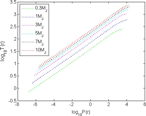
Figure 2 Density distribution inside some initial protoplanets.

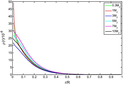
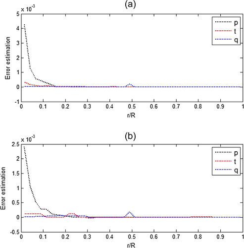
Figure 3 Error estimation of the proposed method through p, q and t with references to the protoplanets with masses $1M_J$ and $10M_J$; (a) for $1M_J$ and (b) for $10M_J$.

4 A description about explicit RKARMS(4,4) numerical technique

The $s-\text{stage}$ RK(4,4) technique for solving the IVP $y^{\prime }=f(x\text{,}y(x))\text{,}{x}_0⩽x⩽x_n$ subject to $y(x_0)=y_0$ can be given by(11) $$y_{n+1}=y_n+h\underset{i=1}{\overset{s}{{{\displaystyle \sum }}^{\text{}}}}{b}_i{k}_i\text{,}$$(11) $\begin{array}{l}\text{where}{k}_i=f(x_n+c_{i}h\text{, }{y}_n+h\underset{i=1}{\overset{s}{{{\displaystyle \sum }}^{\text{}}}}{a}_{ij}{k}_i)\text{,}{c}_i=\underset{j=1}{\overset{s}{{{\displaystyle \sum }}^{\text{}}}}{a}_{ij}\text{,}\\ i=1\text{, }2\text{, }3\text{,}\dots \text{,}s\end{array}$with s dimensional vectors c and b and the $s\times s$ matrix $A(a_{ij})$. 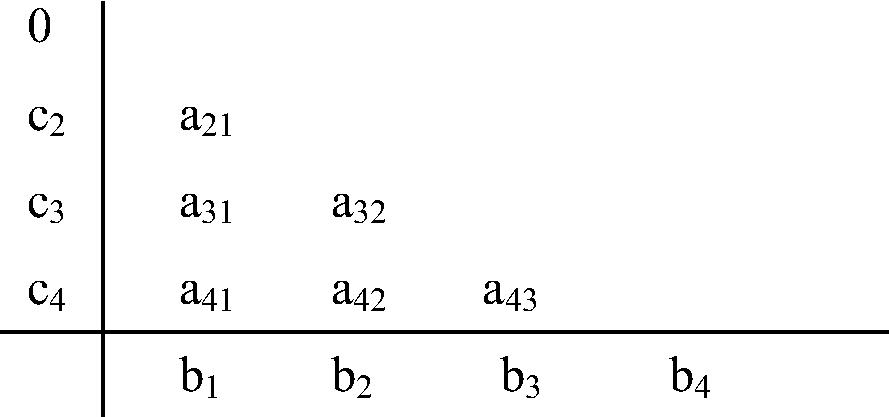A general s-stage RK pair can be written in an array form as

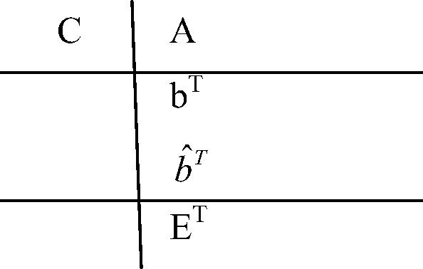
The symbols $C\text{,}A$ and $b^T$ have order s and that $C\text{,}A$ and ${\widehat{b}}^T$ have order $(s+1)$. Using the second method, the value of y at $x=x_{n+1}$ can be expressed as(12) ${\widehat{y}}_{n+1}=y_n+h{\displaystyle \sum _{i=1}^s}{\widehat{b}}_i{k}_i\text{,}$(12) whereas the same for the first method is expressed by Eq. (11(11) $$y_{n+1}=y_n+h\underset{i=1}{\overset{s}{{{\displaystyle \sum }}^{\text{}}}}{b}_i{k}_i\text{,}$$(11) ).

From the embedded form, the LTE may be computed from the formula: $\mathit{LTE}=y_{n+1}-{\widehat{y}}_{n+1}$. It is of interest to note here that LTE leads to control step size.

The four stage method with the Butcher array form is written as follows:

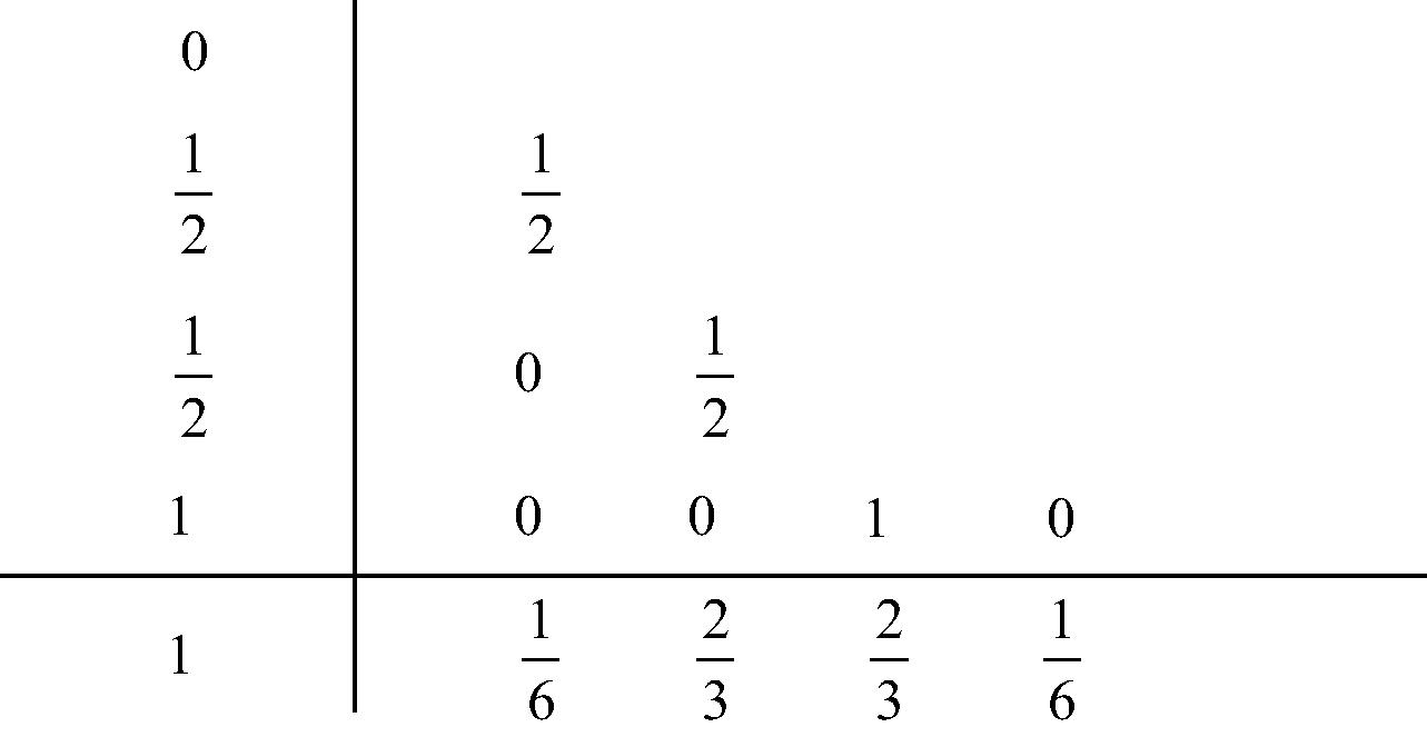
The well-known fourth order RK arithmetic mean (RKAM(4,4)) method can be written in the Butcher array form as follows (see Senthilkumar and Paul, 2012): (13) $y_{n+1}=y_n+\frac{h}{3}\left[\frac{k_1+k_2}{2}+\frac{k_2+k_3}{2}+\frac{k_3+k_4}{2}\right]\text{,}$(13) where$\begin{array}{cc}\hfill & k_1=f(x_n\text{,}{y}_n)\text{,}\hfill \\ \hfill & k_2=f\left(x_n+\frac{h}{2}\text{,}{y}_n+\frac{{\mathit{hk}}_1}{2}\right)\text{,}\hfill \\ \hfill & k_3=f\left(x_n+\frac{h}{2}\text{,}{y}_n+\frac{{\mathit{hk}}_2}{2}\right)\text{,}\hfill \\ \hfill & k_4=f(x_n+h\text{,}{y}_n+{\mathit{hk}}_3)\text{.}\hfill \end{array}$

The fourth order RK method with Butcher array can also be written in the modified form as (see Ponalagusamy and Senthilkumar, 2009)

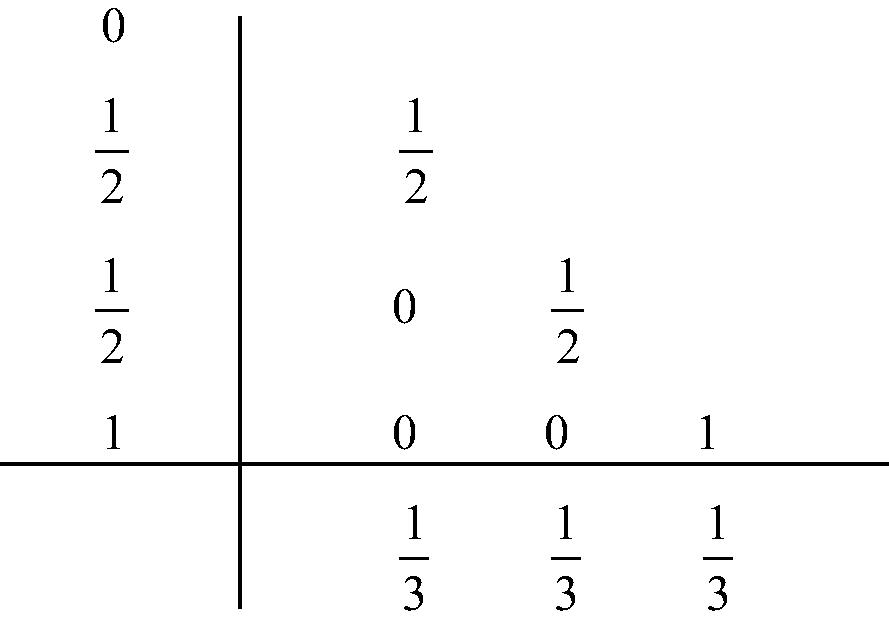
The fourth order RK root mean square (RKRMS(4,4)) method due to Yaakub and Evans (1993) is given by(14) $y_{n+1}=y_n+\frac{h}{3}\left[\sqrt{\frac{k_1^2+k_2^2}{2}}+\sqrt{\frac{k_2^2+k_3^2}{2}}+\sqrt{\frac{k_3^2+k_4^2}{2}}\right]\text{,}$(14) where$\begin{array}{cc}\hfill & k_1=f(x_n\text{,}{y}_n)\text{,}\hfill \\ \hfill & k_2=f\left(x_n+\frac{1}{2}h\text{,}{y}_n+\frac{1}{2}{\mathit{hk}}_1\right)\text{,}\hfill \\ \hfill & k_3=f\left(x_n+\frac{1}{2}h\text{,}{y}_n+\frac{1}{16}{\mathit{hk}}_1+\frac{7}{16}{\mathit{hk}}_2\right)\text{,}\hfill \\ \hfill & k_4=f\left(x_n+h\text{,}{y}_n+\frac{1}{8}{\mathit{hk}}_1-\frac{17}{56}{\mathit{hk}}_2+\frac{33}{28}{\mathit{hk}}_3\right)\text{.}\hfill \end{array}$

It is well-known that combination of RKAM(4,4) and RKRMS(4,4) (Eqs. (⁽¹⁵⁾(15) $y_{n+1}=y_n+\frac{h}{3}\left[\frac{k_1+k_2}{2}+\frac{k_2+k_3}{2}+\frac{k_3+k_4}{2}\right]\text{,}$(15) ⁽¹⁴⁾(14) $y_{n+1}=y_n+\frac{h}{3}\left[\sqrt{\frac{k_1^2+k_2^2}{2}}+\sqrt{\frac{k_2^2+k_3^2}{2}}+\sqrt{\frac{k_3^2+k_4^2}{2}}\right]\text{,}$(14) )) leads to give a new formation of RKARMS(4,4), and is formulated by Ponalagusamy and Senthilkumar (2009) as$\begin{array}{cc}\hfill & k_1=f(x_n\text{,}{y}_n)=k_1^{\ast }\text{,}\hfill \\ \hfill & k_2=f\left(x_n+\frac{h}{2}\text{,}{y}_n+\frac{{\mathit{hk}}_1}{2}\right)=k_2^{\ast }\text{,}\hfill \\ \hfill & k_3=f\left(x_n+\frac{h}{2}\text{,}{y}_n+\frac{{\mathit{hk}}_2}{2}\right)\text{,}\hfill \\ \hfill & k_4=f(x_n+h\text{,}{y}_n+{\mathit{hk}}_3)\text{,}\hfill \\ \hfill & k_3=f\left(x_n+\frac{1}{2}h\text{,}{y}_n+\frac{1}{16}{\mathit{hk}}_1+\frac{7}{16}{\mathit{hk}}_2\right)=k_3^{\ast }\text{,}\hfill \\ \hfill & k_4=f\left(x_n+h\text{,}{y}_n+\frac{1}{8}{\mathit{hk}}_1-\frac{17}{56}{\mathit{hk}}_2+\frac{33}{28}{\mathit{hk}}_3\right)=k_4^{\ast }\text{,}\hfill \\ \hfill \end{array}$(15) $y_{n+1}=y_n+\frac{h}{3}\left[\frac{k_1+k_2}{2}+\frac{k_2+k_3}{2}+\frac{k_3+k_4}{2}\right]\text{,}$(15) (16) $y_{n+1}^{\ast }=y_n+\frac{h}{3}\left[\sqrt{\frac{k_1^{\ast 2}+k_2^{\ast 2}}{2}}+\sqrt{\frac{k_2^{\ast 2}+k_3^{\ast 2}}{2}}+\sqrt{\frac{k_3^{\ast 2}+k_4^{\ast 2}}{2}}\right]\text{.}$(16)

The embedded RKARMS(4,4) method is expressed as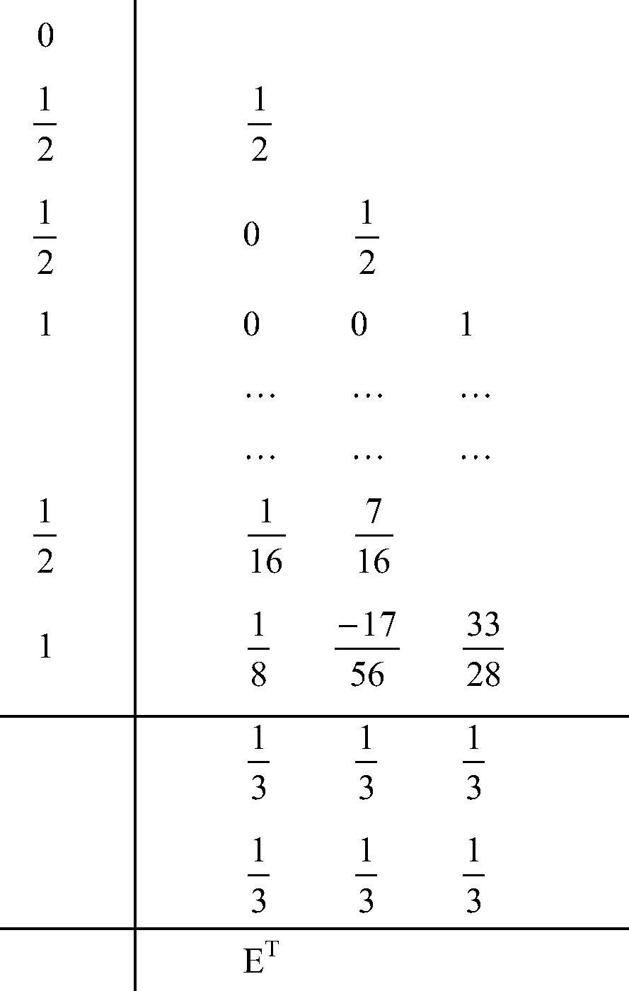$$(17) $\text{Hence,}{b}^T=y_{n+1}^{\mathit{AM}}=y_n+\frac{h}{3}\left[\frac{k_1+k_2}{2}+\frac{k_2+k_3}{2}+\frac{k_3+k_4}{2}\right]\text{,}$(17) (18) ${\widehat{b}}^T=y_{n+1}^{\mathit{RMS}}=y_n+\frac{h}{3}\left[\sqrt{\frac{k_1^{\ast 2}+k_2^{\ast 2}}{2}}+\sqrt{\frac{k_2^{\ast 2}+k_3^{\ast 2}}{2}}+\sqrt{\frac{k_3^{\ast 2}+k_4^{\ast 2}}{2}}\right]\text{,}$(18) and the estimation of the LTE, $E^T=\left|b^T-{\widehat{b}}^T\right|$. In the RKARMS(4,4) method, four stages are required to obtain the solution, which share the same set of vectors $k_1$ and $k_2$ using $b^T$ and ${\widehat{b}}^T$ approximately, but $k_3$ and $k_4$ use $b^T$ while $k_3^{\ast }$ and $k_4^{\ast }$ use ${\widehat{b}}^T$.

4.1 Derivation and error estimation for explicit RKARMS(4,4) method

According to Lotkin (1951), Ralston (1957)and Lambert (1973, 1980), the error estimate for fourth order RK schemes is given $\left|\psi (x_n\text{,}{y}_n:h)\right|⩽(73/720){\mathit{ML}}^4$, where L and M are positive constants. From Eqs. (⁽¹⁷⁾(17) $\text{Hence,}{b}^T=y_{n+1}^{\mathit{AM}}=y_n+\frac{h}{3}\left[\frac{k_1+k_2}{2}+\frac{k_2+k_3}{2}+\frac{k_3+k_4}{2}\right]\text{,}$(17) ⁽¹⁸⁾(18) ${\widehat{b}}^T=y_{n+1}^{\mathit{RMS}}=y_n+\frac{h}{3}\left[\sqrt{\frac{k_1^{\ast 2}+k_2^{\ast 2}}{2}}+\sqrt{\frac{k_2^{\ast 2}+k_3^{\ast 2}}{2}}+\sqrt{\frac{k_3^{\ast 2}+k_4^{\ast 2}}{2}}\right]\text{,}$(18) ), we obtain an estimate of the LTE for the RKARMS(4,4) method as $\mathit{LTE}=y_{n+1}-y_{n+1}^{\ast }$, which may be used to control step size. The LTE for well-known RKAM(4,4) method is(19) $y_{n+1}^{\mathit{AM}}=y_n+{\mathit{LTE}}_{\mathit{AM}}\text{,}$(19) and the LTE for RKRMS(4,4) method is(20) $y_{n+1}^{\mathit{RMS}}=y_n+{\mathit{LTE}}_{\mathit{RMS}}\text{,}$(20) where $y_{n+1}^{\mathit{AM}}\text{and}{y}_{n+1}^{\mathit{RMS}}$ are numerical approximations at $x_{n+1}$ obtained by RKAM(4,4) and RKRMS(4,4), respectively, and ${\mathit{LTE}}_{\mathit{AM}}$ and ${\mathit{LTE}}_{\mathit{RMS}}$ are the LTEs for RKAM(4,4) and RKRMS(4,4), respectively. The difference between $y_{n+1}^{\mathit{AM}}\text{and}{y}_{n+1}^{\mathit{RMS}}$ at $x_{n+1}$ gives an error estimate as(21) $y_{n+1}^{\mathit{AM}}-y_{n+1}^{\mathit{RMS}}={\mathit{LTE}}_{\mathit{AM}}-{\mathit{LTE}}_{\mathit{RMS}}\text{.}$(21)

The LTE for RKAM(4,4) method is given by(22) ${\mathit{LTE}}_{\mathit{AM}}=\frac{h^5}{2880}\left(-24{\mathit{ff}}_y^4+f^4{f}_{\mathit{yyyy}}+2f^3{f}_y{f}_{\mathit{yyy}}-6f^3{f}_{\mathit{yy}}^2+36f^2{f}_y^2{f}_{\mathit{yy}}\right)\text{,}$(22) whereas the LTE for RKRMS(4,4) method can be set to the form(23) ${\mathit{LTE}}_{\mathit{RMS}}=\frac{h^5}{184320}\left(-429{\mathit{ff}}_y^4-64f^4{f}_{\mathit{yyyy}}-48f^3{f}_y{f}_{\mathit{yyy}}-96f^3{f}_{\mathit{yy}}^2-2454f^2{f}_y^2{f}_{\mathit{yy}}\right)\text{.}$(23)

The absolute difference between ${\mathit{LTE}}_{\mathit{AM}}\text{and}{\mathit{LTE}}_{\mathit{RMS}}$ is given by(24) $\left|{\mathit{LTE}}_{\mathit{AM}}-{\mathit{LTE}}_{\mathit{RMS}}\right|=\frac{h^5}{184320}\left(1107{\mathit{ff}}_y^4+128f^4{f}_{\mathit{yyyy}}+176f^3{f}_y{f}_{\mathit{yyy}}+288f^3{f}_{\mathit{yy}}^2+4758f^2{f}_y^2{f}_{\mathit{yy}}\right)\text{.}$(24)

As in Eq. (20(20) $y_{n+1}^{\mathit{RMS}}=y_n+{\mathit{LTE}}_{\mathit{RMS}}\text{,}$(20) ), substituting $f\text{,}{f}_y\text{,}{f}_{\mathit{yy}}$, etc. in Eq. (24(24) $\left|{\mathit{LTE}}_{\mathit{AM}}-{\mathit{LTE}}_{\mathit{RMS}}\right|=\frac{h^5}{184320}\left(1107{\mathit{ff}}_y^4+128f^4{f}_{\mathit{yyyy}}+176f^3{f}_y{f}_{\mathit{yyy}}+288f^3{f}_{\mathit{yy}}^2+4758f^2{f}_y^2{f}_{\mathit{yy}}\right)\text{.}$(24) ), it can be written as(25) $\left|{\mathit{LTE}}_{\mathit{AM}}-{\mathit{LTE}}_{\mathit{RMS}}\right|⩽\frac{6457}{184320}{P}^4{\mathit{Qh}}^5\text{,}$(25) where P and Q are positive constants. If we let $\mathit{TOL}=5.00\times {10}^{-5}$, then by setting $\left|{\mathit{LTE}}_{\mathit{AM}}-{\mathit{LTE}}_{\mathit{RMS}}\right|⩽\mathit{TOL}$, the error control and step size selection can be determined by Eq. (25(25) $\left|{\mathit{LTE}}_{\mathit{AM}}-{\mathit{LTE}}_{\mathit{RMS}}\right|⩽\frac{6457}{184320}{P}^4{\mathit{Qh}}^5\text{,}$(25) ) as(26) $\frac{6457}{184320}{P}^4{\mathit{Qh}}^5<\mathit{TOL}\text{or}h<{\left(\frac{28.54764\times \mathit{TOL}}{P^{4}Q}\right)}^{1/5}\text{.}$(26)

It is pertinent to point out that in the explicit RKARMS(4,4) method with error control program, we choose error estimation as the difference between the results obtained by RKAM(4,4) and RKRMS(4,4) methods. From Eq. (25(25) $\left|{\mathit{LTE}}_{\mathit{AM}}-{\mathit{LTE}}_{\mathit{RMS}}\right|⩽\frac{6457}{184320}{P}^4{\mathit{Qh}}^5\text{,}$(25) ), the error estimation (ERREST) is expressed as (see Table 1)(27) $\text{ERREST}=\left|y_{\mathit{AM}}-y_{\mathit{RMS}}\right|\times \frac{6457}{184320}\text{.}$(27)

Table 1 Comparison of LTE, GTE, and error estimation for RKARMS(4,4) method.

RK-embedded algorithm	Local truncation error (LTE)	Global truncation error (GTE)	Error estimation (ERREST)
Explicit RK-embedded arithmetic root mean square method	${\mathit{LTE}}_{\mathit{AM}}-{\mathit{LTE}}_{\mathit{RMS}}⩽\frac{6457}{184320}{P}^4{\mathit{Qh}}^5=\left|{\mathit{LTE}}_{\mathit{AM}}-{\mathit{LTE}}_{\mathit{RMS}}\right|⩽\frac{6457}{184320}{P}^4{\mathit{Qh}}^5$	$\left|{\epsilon }_n\right|⩽\left(\frac{h^4}{164320\mathit{LD}}\right)\times M\left(e^{\mathit{DL}(x_n-x_0)}-1\right)$	ERREST = $\left|y_{\mathit{AM}}-y_{\mathit{RMS}}\right|\times \frac{6457}{184320}$

5 Discussion on results and conclusion

We have analyzed initial configurations of protoplanets formed via disk instability in the mass range 0.3–10 Jovian masses by a newly proposed explicit RKARMS(4,4) method under approximate zero boundary conditions. Each of the protoplanets has been assumed to be a sphere of solar composition, which is in a steady state of quasi–static equilibrium where ideal gas law holds well, and the energy equation assumes the conduction–radiation heat transport. Fig. 1 depicts initial temperature–pressure profiles of the protoplanets with assumed masses. It can be shown from the figure that after a point little depth from the surface down to the core region, the temperature increases with the increasing mass of the protoplanets, whereas the pressure also increases with their increasing mass except for the protoplanets with masses $1M_J$ and $10M_J$. The results of our calculation agree fairly well with the estimates obtained in the investigations of Helled and Schubert (2008), Paul and Bhattacharjee (2013), and Paul et al. (2013). Fig. 2 shows initial density distribution inside the assumed protoplanets. The figure shows that mater is not distributed uniformly in the atmosphere, and there may have variation in parameters due to gravitational stratification. This is as to be expected for initial unsegregated protoplanets. It can be observed from the figure that the central density of the protoplanet with mass $1M_J$ is higher than the central condensations of the other considered protoplanets and the protoplanet with mass $3M_J$ is found to be rarer concerning both center and surface among all the protoplanets with assumed masses.

Density distribution obtained in the study can be found to be comparable with the ones obtained in the study of Paul et al. (2013). But Helled and Schubert (2008) showed that the surface density of such protoplanets decreases with their decreasing mass and central density increases with their increasing mass. It is pertinent to point out here that, in reality, not a single protoplanet formed by disk instability exists in the literature with its definite structures (Helled and Bodenheimer, 2011; Paul and Bhattacharjee, 2013). However, the system possesses a unique solution suggesting that disk instability is a reasonable hypothesis in planetary formation. The results of our calculation may be important in the study of evolution of extrasolar giant planets. A direct comparison of the results employing the proposed RKARMS(4,4) method is made with the results obtained by the classical Runge–Kutta 4th order (RK(4,4)) method. Only the results for $1M_J$ are presented (see Table 2) because to void space consumption. From the table it is found that the results by the explicit RKARMS(4,4) method are comparable with the results obtained by the RK(4,4) method, which can be seen to be true for all the protoplanetary masses considered. We have evaluated error estimation (ERREST) for the proposed method through the results of the investigation. The results for $1M_J$ and $10M_J$ protoplanets are presented in Fig. 3 for sake of brevity. It is inferred from Fig. 3 that the error estimations are quite reasonable. We have tested our results for varying end points with all the possible step sizes, for which the RKARMS(4,4) method is valid. The results are found to be insensitive to the choice of the end points. In order to compare the computational efficiency of the RKARMS(4,4) method with that of the RK(4,4) method, both the codes were run on the same computer with step size 0.0001. The total computational time was found to be less for the RKARMS(4,4) method (5.978359 s) in comparison with that for the RK(4,4) method (6.065116 s). Thus the RKARMS(4,4) method is found to be more optimal in solving structure equations of protoplanets in comparison with the classical RK(4,4) method with respect to the central processing unit (CPU) time and accuracy.

Table 2 Comparative distribution of thermodynamic variables inside a 1 Jupiter mass protoplanet.

$r/R$	Classical Runge–Kutta 4th order method			New explicit RKARMS(4,4) method
	P (dynes ${\text{cm}}^{-2}$)	T (K)	ρ (g cm^−3)	P (dynes ${\text{cm}}^{-2}$)	T (K)	ρ (g cm^−3)
0.99	$3.8954527\times {10}^{-07}$	$1.6102493\times {10}^{00}$	$6.4512556\times {10}^{-15}$	$3.8954527\times {10}^{-07}$	$1.6102493\times {10}^{00}$	$6.4512556\times {10}^{-15}$
0.90	$5.4656957\times {10}^{-03}$	$1.7901342\times {10}^{01}$	$8.1421533\times {10}^{-12}$	$5.3980124\times {10}^{-03}$	$1.7845786\times {10}^{01}$	$8.2236662\times {10}^{-12}$
0.80	$1.3290122\times {10}^{-01}$	$4.0709788\times {10}^{01}$	$8.7058176\times {10}^{-11}$	$1.3185159\times {10}^{-01}$	$4.0629732\times {10}^{01}$	$8.6930245\times {10}^{-11}$
0.70	$1.0706637\times {10}^{00}$	$7.0401377\times {10}^{01}$	$4.0555650\times {10}^{-10}$	$1.0644930\times {10}^{00}$	$7.0301521\times {10}^{01}$	$4.0473810\times {10}^{-10}$
0.60	$5.6569018\times {10}^{00}$	$1.0969770\times {10}^{02}$	$1.3751831\times {10}^{-09}$	$5.6320485\times {10}^{00}$	$1.0958258\times {10}^{02}$	$1.3770036\times {10}^{-09}$
0.50	$2.4262787\times {10}^{01}$	$1.6205682\times {10}^{02}$	$3.9925723\times {10}^{-09}$	$2.4183268\times {10}^{01}$	$1.6194018\times {10}^{02}$	$4.0165598\times {10}^{-09}$
0.40	$9.2395087\times {10}^{01}$	$2.3108465\times {10}^{02}$	$1.0662455\times {10}^{-08}$	$9.2199260\times {10}^{01}$	$2.3100654\times {10}^{02}$	$1.0713107\times {10}^{-08}$
0.30	$3.2328971\times {10}^{02}$	$3.1822282\times {10}^{02}$	$2.7091933\times {10}^{-08}$	$3.2309502\times {10}^{02}$	$3.1828741\times {10}^{02}$	$2.7168903\times {10}^{-08}$
0.20	$1.0297073\times {10}^{03}$	$4.1622901\times {10}^{02}$	$6.5972184\times {10}^{-08}$	$1.0316243\times {10}^{03}$	$4.1668254\times {10}^{02}$	$6.6508432\times {10}^{-08}$
0.10	$2.7969290\times {10}^{03}$	$4.9796902\times {10}^{02}$	$1.4978163\times {10}^{-07}$	$2.8170636\times {10}^{03}$	$4.9933180\times {10}^{02}$	$1.5070511\times {10}^{-07}$
0.01	$1.0954682\times {10}^{04}$	$6.1391756\times {10}^{02}$	$4.7584900\times {10}^{-07}$	$1.1489201\times {10}^{04}$	$6.2424341\times {10}^{02}$	$4.9146509\times {10}^{-07}$

In our calculation, to make the work simple, the protoplanets are assumed to be spheres of gas and dust where ideal gas law holds well. But the Clapeyron equation of state (ideal gas law) is appropriate only for the gases with no high pressure. Also, in our calculations, we have neglected radiation effect from the parent star. Furthermore, the disturbances from the parent star and the mutual attraction among the protoplanets have not been considered. But future work will be concentrated on the evolution of extrasolar planets formed via disk instability including the factors mentioned above using an appropriate equation of state, where our intention is to implement parallel numerical algorithms that employ large number of processors. The processors perform various tasks independently and simultaneously, thereby, improving the speed of execution of complex programs dramatically. Parallel computers match the speed of supercomputers at a fraction of the cost.

Gour Chandra Paul W as born in Talora, Bogra District, Bangladesh on 20th November 1974. He received his B.Sc. honours degree on Mathematics in 1994, M.Sc. degree on Applied Mathematics in 1995 and Ph.D. degree in Astrophysics in 2005 from the Department of Mathematics, University of Rajshahi, Bangladesh. He was a Post-Doctoral Fellow in the School of Mathematical Sciences, Universiti Sains Malaysia, Pulau Pinang, Malaysia during 2010–2011. Presently he is working as a professor in the Department of Mathematics, Rajshahi University, Bangladesh. He has published many good research papers in peer-reviewed international journals with high impact factor. He is also reviewer and referee for many scientific international journals. His current research interest lies in evolution of Planetary Systems, Numerical Methods, Tide and Storm Surges Modeling and Simulation.

Sukumar Senthilkumar was born in Neyveli Township, Cuddalore District, Tamilnadu, India on 18th July 1974. He received his B.Sc Degree in Mathematics from Madras University in 1994, M.Sc Degree in Mathematics from Bharathidasan University in 1996, M.Phil Degree in Mathematics from Bharathidasan University in 1999 and M.Phil Computer Science & Engineering from Bharathiar University in 2000. Also, he received PGDCA and PGDCH in Computer Science and Applications and Computer Hardware from Bharathidasan University in 1996 and 1997 respectively. He has been awarded doctoral degree in the field of Mathematics and Computer Applications from National Institute of Technology, [An Institute of National Importance-formerly Regional Engineering College], Tiruchirappalli, Tamilnadu, India. He worked as a Post Doctoral Fellow at Universiti Sains Malaysia [An Apex University], School of Mathematical Sciences, Pulau Pinang, Malaysia. Also, he worked as a Post Doctoral Researcher at the Center for Advanced Image and Information Technology, School of Electronics and Information Engineering, Division of Computer Science and Engineering, Chon Buk National University, Jeonju, Chon Buk, South Korea. He worked as a Lecturer/Assistant Professor in the Department of Computer Science at Asan Memorial College of Arts and Science, Chennai, Tamilnadu, India. Currently, he is working as an Associate Professor in the School of Computing Science and Engineering at Vellore Institute of Technology-University, Vellore, Tamilnadu, India. He has published many good scientific research papers in international conferences and in peer reviewed/highly refereed international journals with high impact factor. He has made significant and outstanding contributions to various activities related to research work. He is also an editor, associate editor, editorial board member, advisory board member, reviewer and referee for many scientific international journals. His current research interests lies in advanced cellular neural networks, advanced digital image processing, advanced numerical analysis, methods and algorithms, advanced simulation, modeling and computing. Further, he is actively engaged in other related areas including advanced astronomy, advanced astrophysics and advanced oceanography etc.

Acknowledgments

We would like to thank both the anonymous referees for useful comments that improved the manuscript. The first author also wishes to thank Professor Shishir Kumer Bhattacharjee, Department of Mathematics, Rajshahi University, for discussions and helpful suggestions during the time this manuscript was being prepared. The second author would like to extend his sincere gratitude to Government of India, eternally for providing financial support during doctoral studies via Technical Quality Improvement Programme (TEQIP), Under Ministry of Human Resource Development, to National Institute of Technology [REC], Tiruchirappalli-620015, Tamil Nadu, India. URL: http://www.nitt.edu. Also, the second author wishes to thank Government of Malaysia for offering financial grants during post doctoral fellow scheme to Universiti Sains Malaysia, School of Mathematical Sciences, Pulau Pinang-11800, Penang, Malaysia. URL: http://www.usm.my; Further, the second author express his grateful thanks to Republic of Korea for offering financial grants through second stage of Brain Korea 21 programme for post doctoral researcher scheme to Center for Advanced Image and Information Technology, School of Electronics & Information Engineering, Chon Buk National University, 664-14, 1Ga, DeokJin-Dong, Jeonju, Chon Buk, 561-756, South Korea. URL: http://www.ei.jbnu.ac.kr. and URL: http://www.ei.bk21.jbnu.ac.kr.

Notes

Peer review under responsibility of National Research Institute of Astronomy and Geophysics.