Probing Schrodinger equation with a continued fraction potential

Peer review under responsibility of National Research Institute of Astronomy and Geophysics.

Abstract

We suggest a new perturbed form of the quantum potential and investigate the possible solutions of Schrodinger equation. The new form can be written as a finite or infinite continued fraction. a comparison has been given between the continued fractional potential and the non-perturbed potential. We suggest the validity of this continued fractional quantum form in some quantum systems. As the order of the continued fraction increases the difference between the perturbed and the ordinary potentials decreases. The physically acceptable solutions critically depend on the values of the continued fraction coefficients ${\alpha }_i$.

Keywords:

• Quantum physics
• Schrodinger equation

1 Introduction

The generalized continued fraction is an expression of the form(1) $x=a_o+\frac{b_1}{a_1+\frac{b_2}{a_2+\frac{b_3}{a_3+\dots }}}$(1) where all the $b_i$ are equal to 1 and all the $a_i$ are positive integers in a simple continued fraction. If the iteration (recursion) is terminated after finitely many steps then the continued fraction is said to be finite (terminated). The integers $a_i$ are called the coefficients of the continued fraction. For some history about the continued fractions see (Balzs Knya, 2000).

Fig. 2 The solution of Schrodinger equation for continued fraction potential (4(4) $\frac{h}{2m}{\nabla }^2\psi +\left(E-\frac{{\alpha }_1}{x+\frac{{\alpha }_2}{x}}\right)\psi =0$(4) ) (solid line) and for the $1/r$ potential (dash-dot line). ${\alpha }_1={\alpha }_2={10}^{-5}$.

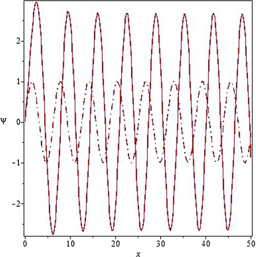
Fig. 3 The solution of Schrodinger Eq. (4(4) $\frac{h}{2m}{\nabla }^2\psi +\left(E-\frac{{\alpha }_1}{x+\frac{{\alpha }_2}{x}}\right)\psi =0$(4) ) for continued fraction potential for ${\alpha }_1={\alpha }_2={10}^2$.

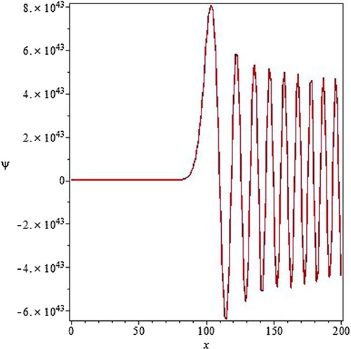
Fig. 4 The solution of Schrodinger Eq. (4(4) $\frac{h}{2m}{\nabla }^2\psi +\left(E-\frac{{\alpha }_1}{x+\frac{{\alpha }_2}{x}}\right)\psi =0$(4) ) for continued fraction potential goes monotonically for some values of the parameters. Here ${\alpha }_1={\alpha }_2={10}^3$.

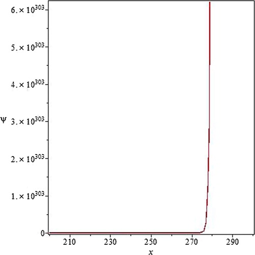
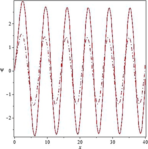
Fig. 5 The solution of Schrodinger Eq. (8(8) $\frac{h}{2m}{\nabla }^2\psi +\left(E-\frac{{\alpha }_1}{x+\frac{{\alpha }_2}{x+\frac{{\alpha }_3}{x}}}\right)\psi =0$(8) ) for the continued fraction potential (solid line) and for the $1/r$ potential (dash-dot line). ${\alpha }_1={\alpha }_2={\alpha }_3=1$.

The continued fraction appears in many contexts in mathematical physics due to its available continuously increasing computational power. continued fraction expansion of special functions (hypergeometric functions and orthogonal polynomials) and solutions of three-term recurrence relations represent important applications. Several algorithms to compute the n-th approximant of a continued fraction have been described in Balzs Knya (2000) (see Figs. 1–6).

Fig. 1 The solution of Schrodinger equation for continued fraction potential (4(4) $\frac{h}{2m}{\nabla }^2\psi +\left(E-\frac{{\alpha }_1}{x+\frac{{\alpha }_2}{x}}\right)\psi =0$(4) ) (solid line) and for the $1/r$ potential (dash-dot line). ${\alpha }_1={\alpha }_2=1$.

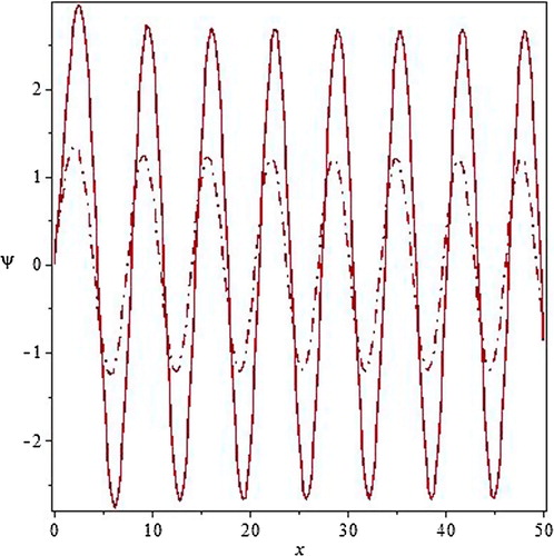
Fig. 6 The solution of Schrodinger Eq. (9(9) $\frac{h}{2m}{\nabla }^2\psi +\left(E-\frac{{\alpha }_1}{x+\frac{{\alpha }_2}{x+\frac{{\alpha }_3}{x+\frac{{\alpha }_4}{x+\frac{{\alpha }_5}{x+\frac{{\alpha }_6}{x}}}}}}\right)\psi =0$(9) ) for the continued fraction potential (solid line) and for the $1/r$ potential (dash-dot line). ${\alpha }_i=1$.

The continued fraction technique has been used in the solution of Schrodinger equation (Biswas and Vidhani, 1973; Mignaco and Miraglia, 1977), the slow neutron scattering calculations (Sears, 1969; Lovesey, 1974) and in strong interaction theory (Zinn-Justin, 1971). In Hnggi et al. (1978), the continued fraction techniques has been used to study the solution of some general physical problems in the field of scattering theory and statistical mechanics. The continued fractions play a role in the study of fractals and dynamical systems (Falconer, 2003; Smeets, 2010). The appearance of continued fraction in perturbation theory has been studied by many authors (Turchi, 1987; Scofield, 1974; Reid, 1967; Cizek and Vrscay, 1984; Swain, 2001).

2 Schrodinger equation with continued fraction potential

The Schrodinger equation for a particle of mass m in a potential $V(r)$ may be written(2) $\frac{h}{2m}{\nabla }^2\psi +\left(E-V(r)\right)\psi =0$(2) with the potential $V(r)=1/r$.

We suppose a perturbed potential in the form of continued fraction as(3) $V(r)=\frac{{\alpha }_1}{r+\frac{{\alpha }_2}{r}}$(3)

For one dimension, Eq. (2(2) $\frac{h}{2m}{\nabla }^2\psi +\left(E-V(r)\right)\psi =0$(2) ) is(4) $\frac{h}{2m}{\nabla }^2\psi +\left(E-\frac{{\alpha }_1}{x+\frac{{\alpha }_2}{x}}\right)\psi =0$(4)

An analytical solution of (4(4) $\frac{h}{2m}{\nabla }^2\psi +\left(E-\frac{{\alpha }_1}{x+\frac{{\alpha }_2}{x}}\right)\psi =0$(4) ) could be written in terms of confluent Heun function HC as(5) $\begin{array}{cc}\hfill & \psi =C_1{e}^{\frac{\mathit{ix}\sqrt{2\mathit{mE}}}{h}}(x+i\sqrt{{\alpha }_2})\mathit{HC}\left(\frac{4\sqrt{2\mathit{mE}{\alpha }_2}}{h}\text{,}1\text{,}-1\text{,}-\frac{4\mathit{im}{\alpha }_1\sqrt{{\alpha }_2}}{h^2}\text{,}\frac{4\mathit{im}{\alpha }_1\sqrt{{\alpha }_2}+h^2}{2h^2}\text{,}\frac{x+i\sqrt{{\alpha }_2}}{2i\sqrt{{\alpha }_2}}\right)\hfill \\ \hfill & +C_2{e}^{\frac{\mathit{ix}\sqrt{2\mathit{mE}}}{h}}(x+i\sqrt{{\alpha }_2})\mathit{HC}\left(\frac{4\sqrt{2\mathit{mE}{\alpha }_2}}{h}\text{,}1\text{,}-1\text{,}-\frac{4\mathit{im}{\alpha }_1\sqrt{{\alpha }_2}}{h^2}\text{,}\frac{4\mathit{im}{\alpha }_1\sqrt{{\alpha }_2}+h^2}{2h^2}\text{,}\frac{x+i\sqrt{{\alpha }_2}}{2i\sqrt{{\alpha }_2}}\right)I\hfill \end{array}$(5)

This analytical solution has been obtained using Maple software. Here I denotes the integral(6) $\int \frac{e^{\frac{-2\mathit{ix}\sqrt{2\mathit{mE}}}{h}}\mathit{dx}}{{(x+i\sqrt{{\alpha }_2})}^2\mathit{HC}{\left(\frac{4\sqrt{2\mathit{mE}{\alpha }_2}}{h}\text{,}1\text{,}-1\text{,}-\frac{4\mathit{im}{\alpha }_1\sqrt{{\alpha }_2}}{h^2}\text{,}\frac{4\mathit{im}{\alpha }_1\sqrt{{\alpha }_2}+h^2}{2h^2}\text{,}\frac{x+i\sqrt{{\alpha }_2}}{2i\sqrt{{\alpha }_2}}\right)}^2}$(6)

This integral can be evaluated numerically. To investigate the numerical solution of (2(2) $\frac{h}{2m}{\nabla }^2\psi +\left(E-V(r)\right)\psi =0$(2) ) we need to know what values of ${\alpha }_1$ and ${\alpha }_2$ lead to a physically acceptable solution i.e. a wave solution.

We set the factor $\frac{h}{2m}$ to 1 for simplicity. This does not change the basic structure of the wavefunctions and their energy when properly scaled. We use the following initial conditions for the wave function and its derivative(7) $\psi (0)=0\text{,}\grave{\psi }(0)=1$(7)

A numerical investigation is always possible to the higher order continued fractional potentials. For example, the solution of;(8) $\frac{h}{2m}{\nabla }^2\psi +\left(E-\frac{{\alpha }_1}{x+\frac{{\alpha }_2}{x+\frac{{\alpha }_3}{x}}}\right)\psi =0$(8) and(9) $\frac{h}{2m}{\nabla }^2\psi +\left(E-\frac{{\alpha }_1}{x+\frac{{\alpha }_2}{x+\frac{{\alpha }_3}{x+\frac{{\alpha }_4}{x+\frac{{\alpha }_5}{x+\frac{{\alpha }_6}{x}}}}}}\right)\psi =0$(9) will also be tested numerically to check the possibility of the wave solution. In the following section we investigate and plot the solutions of Eqs. (⁽⁴⁾(4) $\frac{h}{2m}{\nabla }^2\psi +\left(E-\frac{{\alpha }_1}{x+\frac{{\alpha }_2}{x}}\right)\psi =0$(4) ⁽⁹⁾(9) $\frac{h}{2m}{\nabla }^2\psi +\left(E-\frac{{\alpha }_1}{x+\frac{{\alpha }_2}{x+\frac{{\alpha }_3}{x+\frac{{\alpha }_4}{x+\frac{{\alpha }_5}{x+\frac{{\alpha }_6}{x}}}}}}\right)\psi =0$(9) ) for different values of the parameters ${\alpha }_i$. We compare all the continued fraction solutions with the ordinary solution of the potential $V(r)=1/r$.

3 Numerical results

See Table 1.

Table 1 $\psi$ just increases monotonically for some values of ${\alpha }_1$ and ${\alpha }_2$.

Parameter value
${\alpha }_1$	${\alpha }_2$	Wave solution?
1	1	Yes
0.1	0.1	Yes
${10}^{-2}$	${10}^{-2}$	Yes
${10}^{-5}$	${10}^{-5}$	Yes
10.0	10.0	Yes
50.0	50.0	Yes
${10}^2$	${10}^2$	Yes
${10}^3$	${10}^3$	No
−${10}^3$	−${10}^3$	No
−${10}^{-5}$	−${10}^{-5}$	Yes
−${10}^{-2}$	−${10}^{-2}$	No
−${10}^{-3}$	−${10}^{-3}$	Yes
−1	−1	No
${10}^5$	${10}^5$	No
${10}^6$	${10}^6$	No
${10}^5$	1	No

4 Conclusion

in this paper, the continued fraction concept has been used to perturb the potential in Schrodinger equation and the possibility of physically valid solutions has been investigated. This perturbation of the potential is expected to be important in some quantum systems. As the order of the continued fraction increases the difference between the perturbed and the ordinary potentials decreases. we have investigated many values of the continued fraction coefficients ${\alpha }_i$ where the solutions have been found to be critically depend on the values of these coefficients.

Notes

Peer review under responsibility of National Research Institute of Astronomy and Geophysics.

References

- Balzs Knya, 2000. arXiv:quant-ph/0101040, PhD thesis, University of Debrecen.
- S.N.BiswasT.VidhaniJ. Phys.A61973468
- J.CizekE.R.VrscayPhys. Rev. A3019841550R
- KennethFalconerFractal Geometry: Mathematical Foundations and Applicationsecond ed.2003John Wiley and Sons
- P.HnggiF.RselD.TrautmannZ. Naturforsch.33a1978402
- S.W.LoveseyJ. Phys.C719742008
- J.A.MignacoJ.E.MiragliaZ. Phys. A28019771
- Charles E.ReidQuant. Chem.151967521
- D.F.ScofieldJ. Math.421974383
- V.F.SearsCan. J. Phys.471969199
- Smeets Ionica, 2010. PhD thesis, University of Leiden.
- S.SwainJ. Phys A882001
- Turchi, P., F., 1987. Springer Series in Solid-State Sciences, vol. 58. Springer, Berlin.
- J.Zinn-JustinPhys. Rep. IC197157