Time lapse (4D) and AVO analysis: A case study of Gullfaks field, Northern North Sea

Abstract

A 4D seismic or time lapse survey has been used to investigate the amplitude versus offset (AVO) effects on seismic data in order to identify anomalies in the Gullfaks field for three different reservoir intervals namely the Tarbert, Cook and Statfjord reservoirs. Repeatability analysis has shown that the earlier seismic vintages are the most unreliable for amplitude anomaly analysis as normalised root-mean square (NRMS) values are greater than 50%. This is above the threshold of good and medium repeatability. Fluid substitution models show increases in both P-wave velocity and density for increasing water saturations with a maximum change of 7.33% in the P-wave velocity, and this is in line with predictions from previous work using the Biot - Gassman equations. AVO modelling for the top Tarbert Formation interface produced scenarios of increasing amplitudes with offset for the presence of hydrocarbons, which dim out with 100% brine saturation. This correlates to class III gas sands for different situations of varying Poisson’s ratio across an interface, which has been previously modelled. Two anomalies were identified with one being related to increasing pressure due to water injection correlating to poor permeability around injector well 34/10-B-33. The second anomaly is a case of potential unswept hydrocarbons that displayed a consistent bright spot throughout all of the seismic vintages (in-inlines and crosslines). AVO attribute analysis of this event produced a class II anomaly. However, when comparing near and far offset seismic data, dimming effect was observed producing contrasting evidence. The dimming offset is viewed to have been as a result of poor repeatability values at far offsets. The modelling of the fluid contents in the studied formations to conform to existing literatures justifies the efficacy of the method.

Keywords:

• Time lapse
• AVO analysis
• Gullfaks field
• NRMS and repeatability test

1 Introduction

Time lapse (4D) seismic refers to the repeatability of 3D seismic surveys conducted at some time interval to monitor the production driven changes in hydrocarbon reservoirs. Time lapse (4D) seismic gives an excellent, cheap and reliable opportunity to indirectly image and monitor the flow of fluid in volumetric regions of reservoir that are not included in the expensive wells or well log data (Vedanti et al., 2009). Consequently, the flow of fluid is mapped directly from seismic data rather than mere prediction from fluid simulation (Lumley, 2001). The comparison of a consecutive set of 3D seismic surveys carried out over the same area allows for amplitude and AVO time-lapse effects to be investigated. Variations in amplitudes could potentially be attributed to fluid saturation changes or pressure changes over time as a result of reservoir injection and production mechanisms. The seismic surveys that have been made available are always investigated to find anomalies between various vintages of seismic data. Time lapse is quantitatively able to monitor the pressure injection and pressure depletion (compaction) signals. In most cases, time lapse can distinctively and accurately separate the effect of pressure and saturation changes. This has been made possible by the world-leading marine 4D repeatability (Normalised Root-mean square (NRMS) noise, which is kept at as low as 7%), sparse acquisition systems (enabling high quality 4D from 10-fold data), cheap acquisition and intense effort in simulator synthetic and geomechanical modelling processes (Staples et al., 2006). To extract fluid types or saturations from seismic, crosswell, or borehole sonic data, we need a procedure to model fluid effects on rock velocity and density. Numerous techniques have been developed. However, Gassmann’s equations are by far the most widely used relations to calculate seismic velocity changes because of different fluid saturations in reservoirs. The importance of this grows as seismic data are increasingly used for reservoir monitoring. Interestingly, in time lapse survey, the variation that exists between two seismic vintages acquired at varying time intervals carried out under similar fundamental acquisition conditions provides robust information on the changes in geophysical properties caused by hydrocarbon production. However, in most cases, the subtraction process exhibits extraneous residual energy, which is not characteristically conformed to the time-lapse signal. This spurious residual energy includes acquisition related noise, random noise and signal bandwidth variation. This usually acts as a limitation to the resolution of the time lapse signal (Vedanti et al., 2009).

The aim of this work is to employ a 4D seismic or time lapse survey to investigate the amplitude versus offset (AVO) effects on seismic data in order to identify anomalies in the Gullfaks field for three different reservoir intervals namely the Tarbert, Cook and Statfjord reservoirs. The modelling of the fluid contents in the studied formations to conform to existing literatures justifies the efficacy of the method.

2 Theoretical foundation

The applicability of 4D seismic data requires the rock Physics as well as seismic data analysis. Thus, log analysis, rock Physics measurements and seismic modelling are essential in monitoring the hydrocarbon saturation in reservoirs. Kumar et al. (2006) provided that the dry rock shear modulus $({\mu }_D)$ equals the saturated rock shear modulus $({\mu }_S)$. Gassmann’s Eqs. (⁽¹⁾(1) $K_S=K_D+\mathrm{\Delta }{K}_D$(1) ⁽²⁾(2) $\mathrm{\Delta }{K}_D=\frac{K_M{\left(1-\frac{K_D}{K_M}\right)}^2}{1-\varphi -\frac{K_D}{K_M}+\frac{K_M}{K_F}}$(2) ) basically relate the bulk modulus of a rock to its respective pore, frame and fluid properties, which is often noticed to be affecting amplitude and AVO variations in time lapse surveys(1) $K_S=K_D+\mathrm{\Delta }{K}_D$(1) (2) $\mathrm{\Delta }{K}_D=\frac{K_M{\left(1-\frac{K_D}{K_M}\right)}^2}{1-\varphi -\frac{K_D}{K_M}+\frac{K_M}{K_F}}$(2) where $\phi$ is the formation fractional porosity and $K_M,K_F,K_{D}and{K}_S$ are the bulk moduli of the mineral, fluid, dry rock, and saturated rock frame, respectively. Gassmann’s formulation is straightforward, and the simple input parameters typically can be directly measured from logs or assumed based on rock type as the values for different rocks abound in published literatures. This is a prime reason for its significance in geophysical techniques such as time-lapse reservoir monitoring and direct hydrocarbon indicators (DHI) such as amplitude “bright spots,” and amplitude variation with Offset (AVO). Compressional (V_p) and shear (Vs) velocities associated with densities directly control the seismic response of reservoirs at any single location. Theoretically, P-wave velocity increases, while S-wave velocity decreases slightly with water saturation (Christensen and Wang, 1985). However, both P- and S-wave velocities are generally not the best indicators for any fluid saturation effect. This is a function of coupling between P- and S-wave through the shear modulus and bulk density. In contrast, variation of bulk and shear modulus as functions of pressure indicates that the water-saturation increases the bulk modulus by about 50% while the shear modulus remains constant (Berryman, 1999). The change $\mathrm{\Delta }{K}_D$, is an increment of bulk modulus caused by fluid saturation. Eqs. (⁽¹⁾(1) $K_S=K_D+\mathrm{\Delta }{K}_D$(1) ⁽²⁾(2) $\mathrm{\Delta }{K}_D=\frac{K_M{\left(1-\frac{K_D}{K_M}\right)}^2}{1-\varphi -\frac{K_D}{K_M}+\frac{K_M}{K_F}}$(2) ) indicate that fluid in pores will affect bulk modulus but not shear modulus. As pointed out by Berryman (1999), a shear modulus independent of fluid saturation is a direct result of the assumptions used to derive Gassmann’s equation, which gives the observed changes in time lapse repeatability surveys (Berryman, 1999).

AVO analysis is a technique used by geoscientists to evaluate reservoir’s hydrodynamic/physical properties, lithology and reservoir’s saturants. The properties include porosity, density, velocity and fluid content. However, to obtain optimum results from AVO analysis, well acquired, processed and interpreted seismic data are required. The complexity of the subsurface makes different rocks to have different AVO responses even though the rocks are filled with the same fluid or have the same porosity (Ursenbach et al., 2008). The AVO analyses aim at differentiating light hydrocarbon (oil and gas) sands from brine sands in a structural trap through the effects of changes in rock and fluid properties on amplitude-variation-with-offset (AVO) responses. In the slope-intercept domain, reflections from wet sands and shales fall on or near a trend that is known as the fluid line (Foster et al., 2010). While reflections from the top of sands containing gas or light hydrocarbons show a trend, which is on the average, approximately parallel to the fluid line, reflections from the base of gas sands fall on a parallel trend of the opposite side of the fluid line. The polarity standard of the seismic data is used to decipher whether these reflections from the top of hydrocarbon-bearing sands are above or below the fluid line. Characteristic properties of sands and shales vary and hence reflections from sand/shale interfaces are also displaced from the fluid line. The gap between these trends from the fluid line depends upon the marked difference between the P-wave velocity (V_p) and S-wave velocity (V_s), reflected in the V_p/V_s ratio, which is a function of pore-fluid compressibility. This precisely implies that the distance from the fluid line increases with increasing compressibility (Foster et al., 2010). Reflections from wet sands are closer to the fluid line than hydrocarbon-related reflections. Porosity changes affect acoustic impedance but do not significantly impact on the V_p/V_s contrast. This therefore, implies that porosity changes move the AVO response along trends, which is on the average parallel to the fluid line. The employment of these interpretive techniques to anomalies of the gas sand helps immensely in AVO anomalies in terms of fluids, lithology, and porosity deductions

3 Study location and geological history

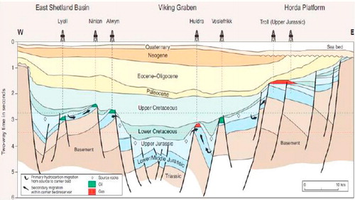
The Gullfaks field is located in the Western flank of the Northern North Sea Viking Graben 175 km northwest of Bergen, east of the Statfjord Field and south of the Snorre Field. The field covers an area of 75 km² and is located in block 34/10 discovered in 1978 and put on production in 1986. The water depth is between 130 m and 220 m with total recoverable reserves estimated as 365 × 106 S m³ (standard cubic metre) of oil and 23 × 109 S m³ of gas (NPD, 2013). The remaining oil has been estimated to be 12 × 106 S m³. The mature Gullfaks field is currently operated by Statoilhydro with total of 275 wells having been drilled in the Gullfaks main field (StatoilhydroHydro, 2007). The Viking Graben rift basin is as result of several phases of extension starting in the Devonian to the Late Jurassic with some localized reactivation influencing the system during the Albian-Aptian period (Fig. 1) (Fossen and Hesthammer, 1998). Regional subsidence occurred from Triassic to Late Jurassic in fluxing the basin with continental to marine sediments with basin fill ceasing by the early Mid Jurassic uplift. There is an unconformity at the base of the Cretaceous (100 Ma time gap) sediment in the Gullfaks field, separating the Upper Cretaceous sediments from Jurassic-Triassic sediments (Statoilhydro, 2007). Splay faulting was the result of the regional tectonic activity with the splay faulting resulting from deformation of the Statfjord Formation towards the Base Cretaceous unconformity. This deformation indicated that the loose sands in the Brent Group responded differently from more compacted strata (Statoilhydro, 2007).

Fig. 1 Regional geology of the Northern North Sea and distribution of hydrocarbon bearing formations within the Lower Jurassic to Paleocene in the Viking Graben (Agustsson et al., 1999; Landrø et al., 1999).

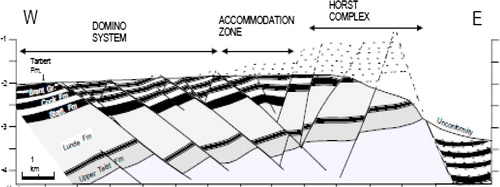
The structural framework of the Gullfaks field is related to the late Jurassic to early Cretaceous rifting system with influences from earlier rifting during the Devonian-Triassic periods (Fossen and Hesthammer, 1998; StatoilhydroHydro, 2007). Such rifting has resulted in general N-S to NNE-SSW fault trends reflecting E-W extension across the rift (Fossen and Hesthammer, 1998). The area is dominated by a domino fault block system located in the western part of the field; this location is where the most important reservoirs of the Brent Group are preserved with faults dipping at $30°$. A horst system is present in the eastern part of the field with a dominant north-south orientation with offsets between 50 and 250 m with throws of almost 500 m (Fig. 2).

Fig. 2 A cross section of the Gullfaks field highlighting the variation between the domino system, accommodation zone and the horst complex trending from West to East (Agustsson et al., 1999).

The three reservoir intervals showcased variations in their respective lithological properties. The uppermost reservoir, the Tarbert Formation, is a subdivision of the Brent Group and has been deposited in a deltaic environment with a thickness variation of 75–105 m. This formation is truncated eastward by the Base Cretaceous unconformity and displays permeabilities of 3–10 D with permeabilities reducing at the base of section three of this formation due to an increase in the shale volume present in this particular section (Statoilhydro, 2007). The Cook Formation can be split into three sections. Section 1 of the Cook Formation (the lowest section) is non-reservoir due to marine shales being interbedded with fine grained sandstone intervals (Fossen and Hesthammer, 1998; Statoilhydro, 2007). The Cook 2 section has poor to moderate reservoir qualities with permeabilities ranging from 2 to 100 mD while the Cook 3 section displays high permeabilities of 100–5500 mD and consists of muddy sandstones, sands and shales (Fossen and Hesthammer, 1998; Statoilhydro, 2007). The Statfjord reservoir consists of 180–200 m of alluvial environment deposited sandstone with an average porosity of 25% and permeabilities reaching 3 D (Vedanti et al., 2009).

4 Materials and method

Seismic data considered from the study area include the 3D seismic for the years of 1985, 1996, 1999, 2003 and 2005 with also an ocean bottom cable survey available for 2005. For the years 1985, 1999 and 2003, the near, mid and far offset data have also been provided and through comparison of these varying offset surveys, the possibility for a refinement of the identification of any anomalies found to deduce their origin is guaranteed. Some proven methods discussed below were employed to achieve the goal.

4.1 Repeatability tests

For reservoir management, time-lapse data is important in evaluating the changes in seismic response due to production (Koster et al., 2000). The seismic survey in 1985 was acquired using a single source and two streamers while the successors used two sources and six streamers but attempted to make consistent the shooting direction and pattern (Landrø et al., 1999). Platforms were permanently installed in the field after the 1985 survey and in order to acquire seismic data beneath them, two vessels in 1995 used an undershoot technique that yielded different azimuthal values (compared to the initial survey) and hence amplitude and timing variations (Landrø et al., 1999; Duffaut and Landrø, 2007). In order to obtain a more reliable result, the horizon of interest in the tests was chosen to be one that is shallow and so unaffected by production.

4.2 Normalized Root Mean Square (NRMS)

NRMS is a common method in estimating repeatability. It is dominant in terms of how sensitive the method is in detecting several differences, namely amplitude, signal to noise ratio, event timing, isochron (time difference between events) and waveform shape (frequency and phase of the wavelet and reflectivity of the events) (Vedanti et al., 2009). The formula for calculating normalised root-mean square (NRMS) was adopted from Kragh and Christie (2002) as in Eq. (3(3) $\mathit{NRMS}=\frac{200\times \mathit{RMS}(\text{base}-\text{monitor})}{\mathit{RMS}(\text{monitor})+\mathit{RMS}(\text{base})}$(3) ).(3) $\mathit{NRMS}=\frac{200\times \mathit{RMS}(\text{base}-\text{monitor})}{\mathit{RMS}(\text{monitor})+\mathit{RMS}(\text{base})}$(3) where monitor is the year recent from the base.

NRMS, which is expressed as a percentage was employed and the results from the calculation was associated with the scale in Fig. 3. NRMS values in the range 130–200% are considered to be data which are anti-correlated i.e. they are 180° out of phase with each other (Kragh and Christie, 2002).

Fig. 3 Scale for NRMS results (Kragh and Christie, 2002).

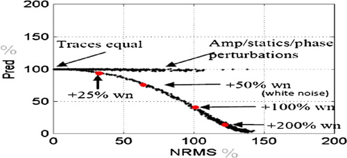
The sensitivity of NRMS was expressed against predictability by adding small perturbations such as random noise, static and phase and amplitude (Fig. 4).

Fig. 4 Cross-plot of predictability and NRMS. Perturbations added do not affect predictability while NRMS gives a significant change (modified from Kragh and Christie, 2002).

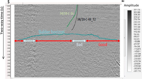
The shallow horizon chosen for NRMS analysis is Balder, which is located at about 1617.9 m True Vertical Depth Subsea (TVDSS), a depth commonly used in the oil industry to represent true vertical depth (TVD) minus the elevation above mean sea level of the depth reference point of the well. In generating the NRMS plots, the monitor and the base were specified. Plots and image maps were used to show the applicability of time lapse in reservoir analysis in the study area. AVO gradient analyses were also used to ascertain the saturants of the reservoirs and the associated gas sand.

5 Results and discussion

Plots for NRMS were generated for sequential years for full offset Pre Stack Time Migration (PSTM) volumes starting with the base as the seismic survey acquired in 1985 (Fig. 5).

Fig. 5 Comparison of NRMS plots for difference of full offset PSTM volumes for consecutive years.

From the repeatability tests, it can be observed that the repeatability increases with the more recent surveys. There are consistent areas in the NRMS plots that show poor repeatability and these correspond to the locations of the permanently installed platforms. The repeatability can also be represented in the difference volume (generated in the NRMS calculation). The seismic section of the difference volume between 2005 and 2003 is shown in Fig. 6. Following the Balder horizon, the noisy and smooth areas in the section correspond to bad and good repeatability respectively.

Fig. 6 Seismic volume section at crossline 2990. Balder horizon at this section shows mainly good repeatability with the bad repeatability corresponding to platform locations.

A distribution plot of the results for the full offset data was created in Fig. 7 and the figure illustrates a shift in the distribution of NRMS for the recent years towards lower NRMS values and this is quantified by the mean values estimated in Table 1.

Fig. 7 Distribution of NRMS results for full offset PSTM data.

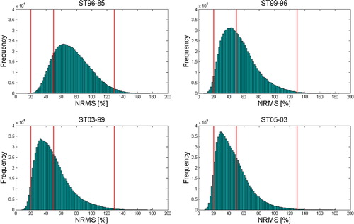
Table 1 NRMS statistics for the full offset PSTM volumes.

Difference volumes	Maximum	Mean	Minimum	Standard deviation
1996–1985	176.43	71.36	15.35	23.40
1999–1996	185.47	49.82	6.52	22.41
2003–1999	178.55	44.51	7.78	21.79
2005–2003	180.09	41.02	7.67	20.55

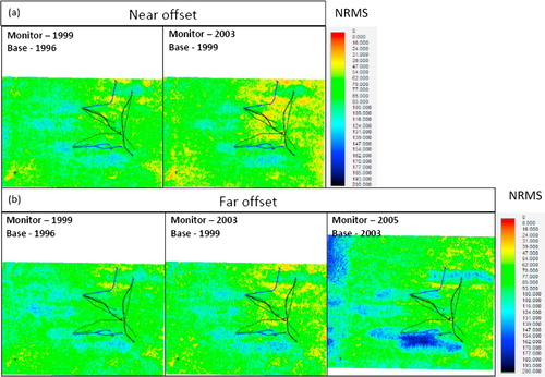
NRMS analysis was performed on near and far offset data as well, to assess the repeatability (Fig. 8). The expectation is that repeatability at near offsets should be much better compared to far offsets as streamer positioning is more manageable closer to the source vessel. Far offset receivers are more susceptible to effects such as weather and currents and so are difficult to control. From the Fig. 8, it can be seen that the repeatability does increase for the near offsets while the far offsets give mostly bad repeatability.

Fig. 8 NRMS plots for (a) near and (b) far offset data. Far offset data show the bad repeatability maintained and then increases for the recent years while near offset increases in repeatability.

5.1 Fluid saturation/substitution

The variations of in-situ fluid saturations impact on the values of P-wave velocities (Vp) and density values of the respective reservoir intervals considered for modelling. The impact of a combination of different saturations of water and oil has been modelled for the Tarbert, Cook (Sections 2 and 3) and Statfjord Formations for wells 34/10–12, 34/10–15 and 34/10–19.

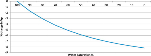
Since the calculation of V_p is dependent on the shear and bulk modulus of the rock that the acoustic wave is propagating through, changes in the bulk modulus directly impact on the value of V_p. From modelling, the change in V_p due to changing water saturations, an increase in comparable values for the relative change in V_p in the Tarbert Formation is remarkably noticeable (Fig. 9). Fluid substitution models show increases in both P-wave velocity and density for increasing water saturations with a maximum change of 7.33% in the P-wave velocity, and this is in line with predictions from previous work using the Biot - Gassman equations (Christensen and Wang, 1985).

Fig. 9 A graph displaying the percentage change in P-wave velocities for varying water and oil saturations in the Tarbert Formation for Well 34/10-12.

The result of modelling the change in P-wave velocity as a function of varying water and oil saturations for the Tarbert Formation in Well 34/10–12 shows that the in situ P-wave velocity decreases as the water saturation decreases and oil present in the formation increases. This trend was seen throughout each of the formations for all the three wells. Modelling of the Tarbert Formation did not reproduce similar changes in V_p compared to the results modelled by Landrø and Strønen (2003). This could be due to using a calculated porosity log as opposed to a constant 30% porosity value. The impact on varying saturations of water and oil on the in situ density was also modelled and the result is shown in Fig. 10 (See Fig. 11).

Fig. 10 A graph displaying the percentage change of the in situ density reading as a result of changing water and oil saturations for the Cook Formation in Well 34/10-12.

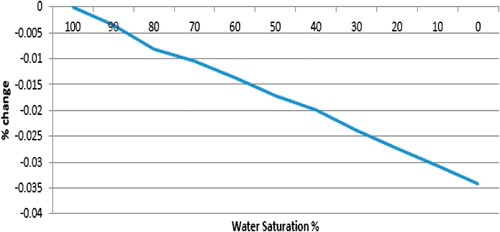
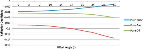
Fig. 11 A graph comparing the variation in amplitude with increasing offset for different fluid substitutions for the top of the Tarbert Formation in Well 34/10-12.

5.2 Amplitude versus offset (AVO) modelling for various fluid substitution scenarios

An AVO model for the top interfaces of each of the reservoirs has been obtained and below is a model for the top of the Tarbert Formation from zero offset to 31° (Far offset angle from ray tracing according to Landrø M., 2007).

The modelling of the top interface of the Tarbert Formation shows that AVO responses from the model correlate well with the models created by Ostrander (1982)and Rutherford and Williams (1978) for the scenarios of a constant Poisson’s ratio across an interface and for a class III gas sand (low impedance sand).

5.3 AVO gradient analysis

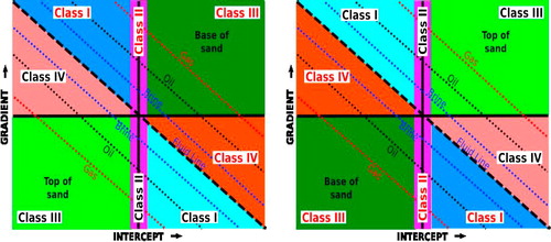
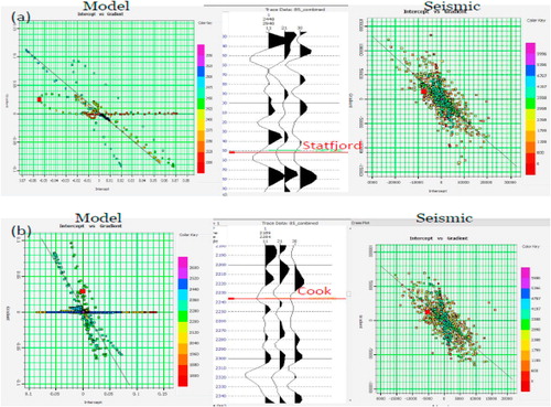
As a matter of fact, the crossplot of intercept and gradient, which is massively employed in amplitude-variation-with-offset (AVO) analysis for hydrocarbon search, was used. The intercept here is referred to as the zero offset or normal incidence reflection amplitude/coefficient of an event while the gradient is the change in reflection amplitude/coefficient with offset at normal incidence (Foster et al., 2010). Reference was made to the fluid line or background trend, the point in which reflection from shales and some wet sands show little or no remarkable contrast in V_p/V_s plot in Fig. 12a by Wayne (2015) for interpretation of changes in clastic reservoir. The positive and the negative transformations show top of sand and the base of sand and the trend of distribution of brine, oil and gas on either side of the fluid line. The classification of gas sand reservoir according to Rutherford and Williams (1989)and Foster et al. (2010) are all shown in Fig. 12a.

Fig. 12a The coordinate transformations (left: positive and right: negative) of the intercept and gradient reflecting the changes in a particular rock property based on the expected behaviour of pore fluid changes in clastic reservoir sequences (modified from Wayne, 2015).

From the study, the AVO gradient analysis was performed on synthetic data for each of the reservoirs for the 1999 seismic vintage. Each reservoir was modelled for a pure brine, oil and gas cases at each well. Fig. 12b shows the comparison between the synthetic and actual seismic analysis for a pure brine case in the Tarbert Formation.

Fig. 12b Comparison between gradient-intercept plot for synthetic and seismic analysis at the Tarbert Formation (Colour code reflects amplitude for different fluids substitutions).

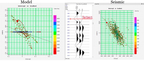
The result shows that for the gradient-intercept plot model, the anomaly (reddish in colour) on the crossplot falls within class 1 gas sand while on the seismic gradient-intercept plot, the anomaly falls on the fluid line. According to Rutherford and William’s classification (1989), all hydrocarbon filled rocks must fall within classes III and IV, the low acoustic impedance. However, comparing our model and seismic results given in gradient-intercept plot to Fig. 12a, it could be deciphered that the positions of anomalies (on model and seismic) fall within the wet trend. Since reflections from wet sands are closer to the fluid line than hydrocarbon-related reflections according to Foster et al. (2010), the observed anomaly on the model and seismic results in Fig. 12b is caused by pure brine and is not hydrocarbon related.

The same scenario was performed for the tops of the Statfjord and Cook reservoirs. Fig. 13 shows the outcome respectively. Modelling at the Statfjord top yields anomaly reflecting hydrocarbon response as the observed anomaly falls away from the mudrock line while for the Cook; the response is similar to that of the Tarbert. Seismic analysis in Tarbert Formation gives results consistent to a pure brine scenario (anomaly falls near the mudrock line).

Fig. 13 Comparison between AVO synthetic and seismic modelling for the top of the (a) Statfjord and (b) Cook reservoirs. (Colour code reflects amplitude for different fluids substitutions).

5.4 Sweep direction

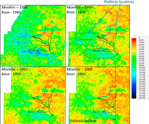
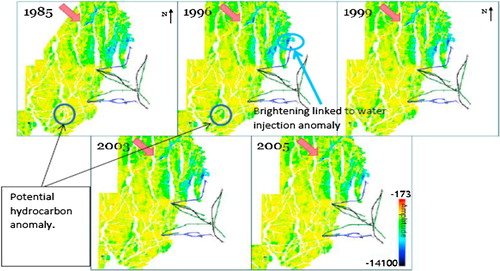
The general sweep direction has been deduced by generating amplitude maps (for each vintage) and analysing the direction in which the high amplitude hydrocarbons drain. Fig. 14 gives the amplitude maps for the Tarbert Formation. Following a section containing hydrocarbons (as indicated by red arrow), it is observed that the amplitude response dims in the South-east direction, towards the production and injection wells. This effect is assumed to be due to the water injection in the well, which eases oil recoverability in reservoirs.

Fig. 14 Amplitude maps for the Tarbert Formation for different vintages. High amplitudes due to the hydrocarbons show dimming in the South-east direction.

5.5 Anomaly investigation

Comparison of the seismic response from the 3D surveys acquired in 1985 to 2005 identifies changes in the fluid saturation, which implies changes in the reservoir pressure. This is due to hydrocarbon production, water injection or gas flooding into the reservoirs. The process therefore, shows various types of anomaly responses such as brightening or dimming effects on the seismic sections. Based on rock Physics and amplitude analyses, two anomalies are identified as shown in Figs. 15 and 16. The analysis involves critical examination of full offset prestack time migration (PSTM), near and far offsets of seismic sections.

Fig. 15 Anomalies identified in the Gullfaks field (Left: anomaly related to water injection in Cook reservoir; Right: Hydrocarbon anomaly in Tarbert reservoir).

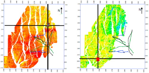
Fig. 16 Water injection anomaly in the Cook Formation for the years considered.

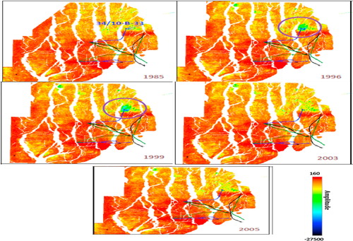
From the generated maximum trough amplitude map for the top Cook Formation for each vintage, the bright spot around the injection well 34/10-B-33 was identified (Fig. 16). The bright spot was then studied in more detail in inline and crossline seismic sections (Figs. 17 and 18). The anomaly shows that the bright spot began to appear in 1996 vintage and this is consistent with the fact that injection into the Cook Formation began in 1995. As previously mentioned, the injection history of the reservoir indicates that injection ceased in 2003 due to water leakage into the Tarbert Formation (Statoil Hydro, 2007). This effect therefore, caused the anomaly to dim at the years after injection halted. The anomaly shows that the bright spot starts to appear in 1996 vintage and this is consistent with the fact that injection into the Cook Formation started in 1995. Fig. 19 shows the comparison between near and far offsets of the anomaly in the inline direction and it shows dimming effect at far offset. The anomaly result corresponds with rock Physics analysis where the increase in pore pressure dims with offset. Pressure builds up around the injection well is as result of the relatively heterogeneous reservoir condition (Feng and Bancroft, 2006; Landro, 2001).

Fig. 17 Identified anomaly related to water injection at well 34/10-B-33.

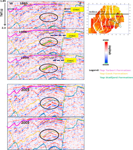
Fig. 18 Identified anomaly related to water injection at well 34/10-B-33 in crossline 2920.

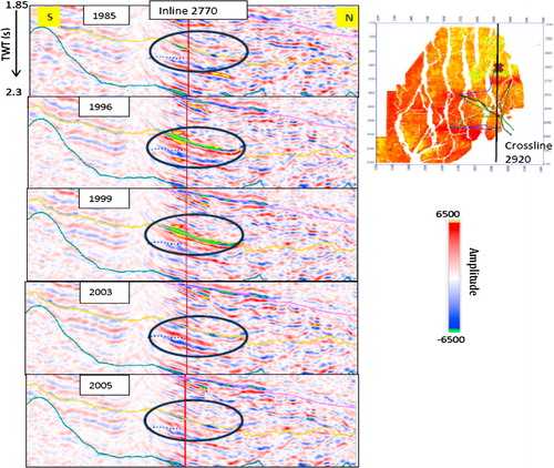
Fig. 19 Comparison of brightening in Near- and Far-offset seismic sections (The location of inline 2770 is shown in Fig. 14).

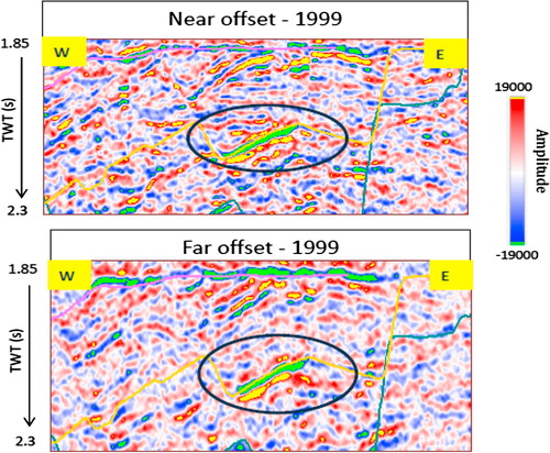
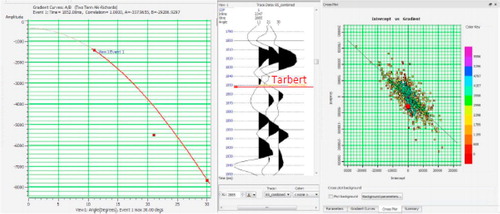
Amplitude maps generated for the top Tarbert Formation shown in Fig. 14 are presented for the years. As seen, there is a consistently high amplitude response at certain locations. An investigation was made to find any possible hydrocarbons near the dry well 34/10–12. A potential hydrocarbon related anomaly was found in inline 2208 where comparison between the different vintages reflects consistently bright amplitude (Fig. 20). This was followed up by cross checking the anomaly on crosslines as well as near and far offset seismic sections (Figs. 21 and 22). Existing anomaly in inline and crossline sections suggests that the identified event is hydrocarbon accumulation. However, study of the near and far offset sections shows that the anomaly dims with offset. This result contradicts with AVO modelling which suggests brightening with far offsets. However, when AVO analysis was done on this location, a class II hydrocarbon reservoir shown in Fig. 23 was realizable.

Fig. 20 Identified anomaly related to possible hydrocarbon accumulation identified on inline 2208.

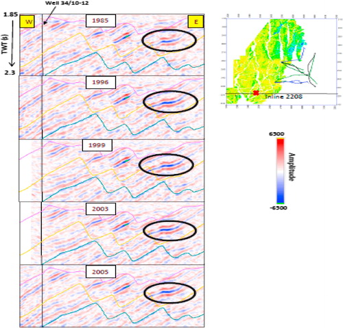
Fig. 21 Identified anomaly related to possible hydrocarbon accumulation identified on crossline 2450.

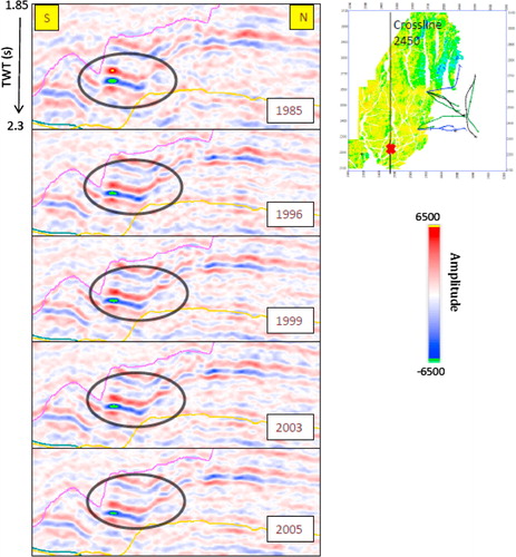
Fig. 22 Comparison of Near and Far offset seismic sections for identified possible hydrocarbon accumulation. The location of inline 2208 is shown in Fig. 20.

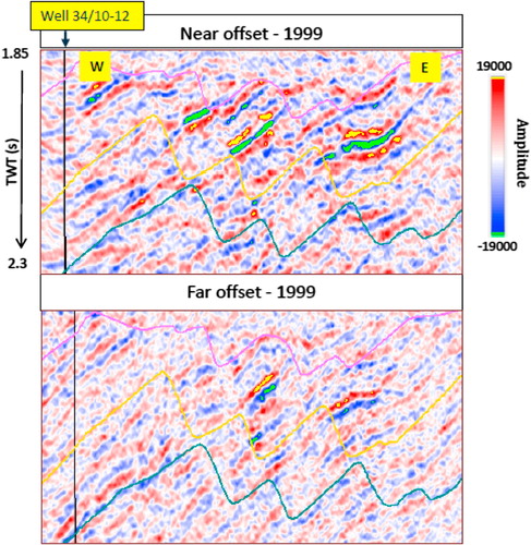
Fig. 23 AVO gradient analysis on the potential hydrocarbon anomaly giving a hydrocarbon result (Colour code reflects amplitude for different fluids substitutions).

6 Conclusions

Fluid substitution modelling has proved for the well data available that the P-wave velocity and density of the three formations increases with increasing water saturations. The Tarbert Formation showed the greatest sensitivity to changes in fluid substitution as a result of having the highest porosity of the three reservoirs. AVO modelling of the Tarbert Formation also produced consistent results that agreed with previous modelling by Ostrander (1982) for a constant Poisson’s ratio across an interface and modelling by Rutherford and Williams (1989) for class III gas sand. The sweep direction of the Tarbert Formation has been deduced to be in a SE direction through analysis of trough amplitude maps between all the five seismic vintages. A low permeability has also been inferred around injector well 34/10-B-33 as amplitude increases throughout the consecutive seismic vintages. Two amplitude anomalies have been investigated and they have been used to deduce the origin of the anomaly. The first anomaly has been attributed to a pressure increase around the injector well, 34/10-B-33. However, it has been inferred to be water -induced as it lies below the oil water contact (OWC) and shows a slight dimming effect between near and far offset seismic datasets. The second anomaly has been deduced as being unswept hydrocarbons situated in the southwest section of the survey region. Consistent amplitudes between seismic vintages were seen with gradient and attribute analysis of the event reinforcing the initial hypothesis that it is a hydrocarbon anomaly and not simply a noise attributed anomaly. However contrasting evidence is seen through comparison of near and far offset data for the seismic datasets of 1999, where significant dimming effect of the reflection event can be seen. These contrasting pieces of evidence suggest that this is only a possible region of unswept hydrocarbons. The analyses of time lapse and AVO have really contributed to the estimation the saturants of the Tarbert, Cook and Statfjord Formations.

Acknowledgements

We gratefully acknowledge the Statoilhydrohydro Company for giving the first author, the data analysed in this paper. We also acknowledge Dr Jenny Collier of the Department of Earth Science and Engineering, Imperial College, London for supervising the first author in his M.sc project that this work is evolved.