Uncertainty, ambiguity and adaptive flood forecasting

Abstract

Reliable long-term flood forecasts are needed because floods, among environmental disasters worldwide, do most damage to lives and property, a problem that is likely to increase as climate changes. The objective of this paper is to critically examine scientific approaches to flood forecasting under deep uncertainty and ambiguity as input to flood policy, and to explore alternative approaches to the development of better forecasts along with the necessary organizational support. This therefore a paper on science policy Aleatory (i.e. frequentist) probability estimates have dominated the science, attached to which are irreducible uncertainties. The lower priority given to finding a physical theory of floods means that ambiguity is high, particularly in relation to choosing a probability density function for forecasting. The historical development of flood forecasting is analyzed within the Uncertainty-Ambiguity Matrix of Schrader, S. Riggs, W.M., and Smith, R.P. (1993). Choice over uncertainty and ambiguity in technical problem solving. Journal of Engineering and Technology Management, 10, 13–99 showing that considerable uncertainty and ambiguity exist and are likely to continue. The way forward appears to be a mix of: broadening the information input to forecasts by engaging many disciplines, Bayesian analyses of probabilities, scenario analyses of catastrophic floods based on all available evidence, and adaptive forecasting in the face of climate change.

Keywords:

• Flood forecasting
• Uncertainty
• Ambiguity
• Scenarios
• Organizational repsonses

1 Introduction: aims and background

Floods are the most destructive of all environmental disasters worldwide and the magnitude and possibly frequency of floods is likely to rise as Earth warms and the hydrological cycle is enlivened (Sayers et al., 2013). Given the worldwide significance of floods, flood forecasting needs to be as robust as possible, and able to cope with a changing climate. The motivation for this paper is to improve forecasts.

In most countries the analytical input to policies to mitigate and/or control flood threat and vulnerability has been traditionally based on natural science, often with an engineering objective, but has been balanced more recently by input from the social sciences (Malamud & Petley, 2009). This input is an example of Laswell's (1970) knowledge in the policy process, an issue of growing importance as predictions are increasingly sought (Sarewitz & Pielke, 2000). This approach to flood mitigation is identified by Nobert et al. (2015) as rooted in the modern desire to control the future. They also see flood forecasting as part of a ‘…general shift toward anticipatory forms of governance based on science and risk.,’ showing that advances in quantitative science are necessary for modern risk governance. More generally Nobert et al. (2015) argue that risk assessment has become a powerful instrument of modern governance.

Hydrologists and engineers have expended significant energy to understand how to cope with uncertainties in flood forecasts, a general characteristic of risk assessment research. Though sociologists of organizations claim that risk-based governance is incompatible with institutional values, structures and procedures (Hood, Rothstein, & Baldwin, 2004), quantitative anticipation of future floods and flood damage are still firmly embedded in flood forecasting, A critical examination of quantitative flood forecasting is warranted because of its central place in flood mitigation policy and because the uncertainties and ambiguities associated with flood forecasting, especially for the most extreme floods, are large and may even lead to delusion. There is also a school of thought that doubts the efficacy of forecasting, suggesting instead that anticipation may be best accomplished by scenario analysis.

In this paper the methods and uncertainties of flood forecasting are critically examined within the Uncertainty-Ambiguity Matrix of Schrader, Riggs, Robert, and Smith (1993) and alternatives to current practice suggested. Uncertainties are both aleatory and epistemic arising from a lack of information, while ambiguity arises from a lack of clarity about the problem structure, particularly the variables involved and their interrelationships. Schrader et al. (1993) also make the important point that different organizational structures are required to deal with uncertainty and ambiguity, a topic to be returned to later in this paper.

Flood risks can be decomposed into the threat of flood and vulnerability to flood. When a large flood occurs, in a location where vulnerability (for a detailed account see Phillips, Thomas, Fothergiill, & Blinn-Pike, 2010) is high, a disaster is the result. Therefore disaster risk is best thought of as a combination of the factors that make people vulnerable to threats (also called hazards) (Wisner, Blaikie, Cannon, & Davis, 2004). In this paper only forecasting of flood threats is considered. Forecasts are of two kinds. First the operational or real-time forecast when a flood is likely or has begun, involving, in the most sophisticated cases, meteorological forecasts, hydrologic modeling, warnings, evacuations, and recovery plans. In simpler cases warnings are issued based on river levels upstream and travel times for the flood wave are made publically available on signboards, on television or radio, and recently through social media and mobile phones. The second kind of forecast aims to estimate the probability of floods of a particular magnitude for each year in the foreseeable future as an input to infrastructure design, flood-prone land zonation, and flood evacuation planning. These probabilistic forecasts are thought to apply over the lifetime of a major structure such as a dam. The time domains of the two kinds of forecast are therefore hours to days (and sometimes months) in the first case and years to many decades in the second case.

Flood Risk Management (FRM) is gradually replacing Flood Control (FC) as those responsible for flood policy and implementation broaden their perspectives (Plate, 2002; Sayers et al., 2013). FC is an authoritarian approach based on engineering and command and control procedures that are often forced on society, such as embankments to ‘control’ floods. Vulnerability is assumed to be reduced by the policies and measures of (usually) government agencies, with varying degrees of investigation. The uncertainties and ambiguities attached to FC are therefore about the design of engineering works with some attention to the probability of floods of particular magnitudes, and there is little ambiguity in the minds of its proponents. In contrast FRM takes account of the social and political environment in which flood management occurs and decisions are taken, and the views of society are taken into account, usually within the constraints of a particular objective such as limiting damage from floods. FRM allows flood disaster risk to be considered in the same framework as other disasters such as those involving earthquakes. FRM uncertainties are therefore associated with both threat and vulnerability, and ambiguities arise if the relationships between them are unclear; an issue not explored here.

This paper will only address the ambiguities and uncertainties associated with the second kind of flood forecasting, namely that which aims to estimate the probability of floods over the foreseeable future rather than real-time forecasting. This is because the two kinds of flood forecasting involve different types of science and policy for forecasting. Vulnerability will also not be included because of the constraints of space. But this relatively narrow focus should not be construed as an endorsement of what Phillips and Fordham (2010) describe as the Dominant View that they claim sees extreme geophysical events as the primary cause of disasters and science and technology as the primary solutions, to the exclusion of political, social and economic dimensions.

2 Flood forecasting: methods and problems

The standard analysis of flood threat, beginning with Fuller (1914), is to determine the probability of a flood of a particular magnitude and return period (RI). The simplest expression of RI, or the average recurrence interval between events, is where N is the number of years of record and n is the number of flood events. When magnitudes are known where n is as above and m is the magnitude ranking.

It is immediately obvious that this analysis requires good historical records. In fact, the small number of extremes in gauged records makes longer histories critical to the endeavor. Calculation of the probability of a flood of a particular value of m and RI is traditionally achieved by assembling all of the peak flows, measured at a stream gauging station, and fitting a statistical function such as the Pearson Type III distribution, the Gumbel distribution or the Generalized Extreme Value distribution assuming statistical stationarity where the mean and variance of peak flow series are constant and random over time. A statistical goodness of fit test is used to choose the best distribution (Millington, Das, & Simonovic, 2011) although in some countries a particular distribution is mandated (e.g. the Pearson Type III in the USA) without a sound basis for choice in the physics of the system (see Dooge, 1986). The lower the annual probability the less is known about the appropriate distribution (Taleb, 2013).

When a Probability Distribution Function (PDF) is used to calculate RIs for low probability events, extrapolation beyond the range of the measured data introduces uncertainties over and above those attached to each measured flow. And there are other sources of uncertainty: there is a 65% chance that a flood will occur within its return interval, assuming independence of flood events (Scheidegger, 1975) and therefore a 35% chance that it will not; empirical estimates of the 100 year Return Interval flood (see below) requires at least 100 years of measured flows, but this is rarely available, hence the need for extrapolation, but none of the commonly used PDFs can adequately represent the upper tails of the probability distributions (Gupta, Troutman, & Dawdy, 2007).

For risk analyses over a large area a method of spatial extrapolation is used to estimate flood flows for ungauged streams for different RIs. For example, Eash, Barnes, and Veilleux (2013) used generalized least squares regression to estimate flood magnitudes for RIs of 2, 5, 10, 25, 50, 100, 200 and 500 years producing mean standard errors of prediction from 19 to 47%. RIs are now usually expressed as Annual Exceedance Probabilities (AEPs; the floods that have a particular probability of being equaled or exceeded in any year) because they are easier to communicate outside technical circles (USGS, 2010). A RI of 500 years corresponds to an AEP of 0.2% (or a probability on a scale of 0–1 of 0.002); that is, a flood with a 0.2% probability of occurring or being exceeded in any year.

The development of complexity ideas has led to a new approach to flood frequency statistics. Malamud and Turcotte (2006) showed that floods approximate power law (fractal) frequency-magnitude relationships along with other environmental phenomena such as volcanic eruptions, forest fires, landslides, and asteroid impacts. A power law flood frequency distribution takes the form where Q(T) is the maximum discharge with a recurrence interval of T years, and C and α are regression coefficients. The parameter α is the slope of a log (Q) versus log (T) plot. In addition a flood-frequency factor F is defined as the ratio of the peak discharge over a 10-year interval to the peak discharge over a 1-year interval and, because of the scale invariance of the power law relationship, F is also the ratio of the 100 year peak discharge to the 10 year peak discharge which reduces to

Malamud and Turcotte (2006) make the important point that it is not yet clear if a power law distribution is superior to other distributions, but it is certainly more conservative. That is, ‘…the fat-tailed power-law distribution will consistently provide higher flood-frequency estimates than the much thinner-tailed log-Pearson Type 3, and other thin-tailed probability distributions’. To add weight to this statement they note that in the USA a fractal analysis of 100-year floods suggests that they occur more frequently than estimated using other distributions. This could be a result of clustering of events in a non-stationary series or because flood peaks are fractally distributed.

In an attempt to understand the power law relationship these authors also speculate that it is the result of a cascade of metastable clusters such as storm cells, analogous to the spread of a fire between clusters of trees. But Gupta et al. (2007) posit that it is the scale invariant (or self-similar) structure of the drainage network of a river catchment that transforms the non-scale-invariant processes of water transport into a scale invariant power law relationship. They go further to suggest that the structure of the drainage network will remain essentially constant under climate change and therefore the key to predicting catchment responses to climate change is to understand the links between climatic factors and the power law relationships, and presumably use the output of global climate models superimposed on catchment drainage networks to calculate the effects of climate change. If this is possible it provides a way around the non-stationarity problem (Dawdy, 2007).

In the examples given above all peak flows are used in one analysis to derive the AEP irrespective of the causes of the floods and therefore differences between flood AEPs under different climatological conditions. Additional information can be gained by taking account of the climatological conditions that cause floods. There are many examples of this approach but only that by Kiem, Franks, and Kuczera (2003) will be referred to here. In many parts of the world, including much of Asia, the El Niño-Southern Oscillation (ENSO) is a major climatological control on floods, and markedly so in Australia. Kiem et al. (2003) showed that multi-decadal epochs of both enhanced and reduced flood threat are the result of modulation of ENSO by the Interdecadal Pacific Oscillation (IPO), a low frequency variation in Pacific Sea Surface Temperatures that is causally related to climate fluctuations on the same time scale. Cold ENSO events (La Niña events) increase flood risk in parts of Australia, the magnitude and frequency of which are affected by modulation by the IPO. Using a regional flood index from 1920 to 2000 it was shown that floods with an AEP of 0.01 were about two orders of magnitude larger in La Niña years than during El Niño years. There was a slightly smaller difference for AEPs of 0.1. When the IPO was positive (index <−0.5) floods were two orders of magnitude larger than when the IPO was positive (index > 0.50). Also the regional flood index is much higher during La Niña years when the IPO is negative by comparison with all other La Niña years. The AEP of 0.01 is most likely to occur when the IPO is negative, a conclusion consistent with temporal clustering of floods.

Kiem et al. (2003) drew the important conclusion that assuming an unchanging climate, as implied by analyses of all peak flows together, is inadequate. While this is a powerful conclusion, how can it be used for prognostic purposes? The most obvious way is by monitoring the IPO index, but calculation of AEPs of low probability will require global climate models that can accurately simulate ENSO and the IPO. This is currently difficult (CapotondI, Guilyardi, & Kirtman, 2013; Collins et al., 2010) and may never be.

In addition to the calculation of AEPs, the armory of technical tools available to the decision maker has been augmented by calculation of the Maximum Probable Flood (MPF) and the Maximum Flood Envelope (MFE). The PMF is the theoretical largest flood that is physically possible (Francés & Botero, 2003) and is generated using a hydrologic model from the Probable Maximum Precipitation (PMP) which is ‘The greatest depth of precipitation for a given duration meteorologically possible over a given size storm area at a particular location at a particular time of year, with no allowance made for future long term climate trends’ (WMO, 1986). The PMP is based on observed precipitation events that are assumed to capture the maximum physically possible extremes (Jakob, Smalley, Meighen, Xuereb, & Taylor, 2009) but there is no physical model that enables its calculation and therefore a test of the empirically derived estimate. The PMF is generally not found in gauged records because they are too short, extrapolation using a PDF fit to gauged data has a large uncertainty, and most of the commonly used extreme distribution functions have no upper limit and therefore should be inapplicable. However, Francés and Botero (2003) have used probability distribution functions with upper and lower bounds to estimate the PMF.

The MFE is an empirical plot of the largest Floods Of Record (FOR) against catchment area for a particular region, or the world, with the form where x _i is the annual maximum flood at site i from the FOR, A _i is the catchment area at site i, a is the intercept, and b is the slope. This function can be compared with the same function for the PMF. Vogel, Matalas, England, and Castellarin (2007) showed that for 226 catchments in the USA, with areas ranging over five orders of magnitude, the PMF is on average 2.5 times larger than the FOR because of the assumptions that are required to derive PMFs from PMPs. But in some cases actual extreme precipitation has exceeded the PMP (Bewsher & Maddocks, 2003) suggesting that the estimates of the PMP are not robust and different methods used to calculate the PMP (see Jakob et al., 2009) give different results that must in turn affect calculations of the PMF.

A limitation of the MFE is that in most cases the function has not been assigned an AEP, something that Graham (2000) sees as essential to estimate costs and benefits of modifications to dams, for example, to meet the requirement that dam spillways can handle the PMF; even though theoretically the PMP has no exceedance probability. Vogel et al. (2007) developed a method to calculate the Envelope Exceedance Probabilities (EEPs) for MFEs using different PDFs and record length weighting. Despite improvements on previous studies their estimated EEPs for FOR of 6.11 ± 5.94 × 10⁻⁴ (a mean probability of 0.000016) has a coefficient of variation of 97% and the EEP for PMFs is 25.51 ± 32.96 × 10⁻⁴ (a mean probability of 0.0000039) with a coefficient of variation of 129%. These large uncertainties do not permit accurate predictions but as input to decision making they possibly capture the correct order of magnitude, assuming that the flood magnitudes in the EEPs are really the maxima.

The assumption of stationarity in flood series, and in the PMF, introduces uncertainties when long histories and future climate change are considered. Milly et al. (2008) declared that ‘Stationarity is Dead” because of human-induced climate change; that is, ‘the idea that natural systems fluctuate within an unchanging envelope of variability’, that can be modeled for forecasting purposes, and that climate variations and human disturbances of catchments have been sufficiently small to allow stationarity-based design. They urge hydrologists and policymakers to use stochastic methods to describe the temporal evolution of PDFs, combine gauged records with palaeoflood records (more on this later), and maintain hydroclimatic monitoring of the highest quality. Pielke (2009) takes the argument much further, arguing that stationarity has always been dead and that we should give up the ‘…fanciful notions of foreseeing the future as the basis for optimal actions’, a position put even more forcefully, and elaborately, by Taleb (2013). That stationarity has always been (or is mostly) dead is clear from many analyses of palaeoflood and historical flood records (e.g. Wasson et al., 2013).

This critical view is given more weight when it is realized that the PMP is both controversial and likely to be non-stationary. Controversy is in several forms: the existence of a PMP is questioned; the accuracy of a PMP estimate is dependent upon the length and spatial distribution of the records because the PMP is not physically based (Douglas & Barros, 2003); different methods of calculation produce widely varying Exceedance Probabilities (an order of magnitude in one case; Douglas & Barros, 2003); the estimates should be place-based rather than global (e.g. Desa & Rakhecha, 2007); the PMP has often been exceeded showing that the calculations are not robust (Koutsoyiannis, 1999); the lives and property saved by using a PMP as the input to calculation of a PMF as the design flood for dam spillways for example are far outweighed by the costs (Graham, 2000); and the use of a PMP removes responsibility from decision makers and is ethically questionable because it implies that engineering designs are free from risk (Benson, 1973).

Non-stationarity of the PMP and the PMF are particularly important in the face of climate change. To investigate the role of climate change on the PMP Jakob et al. (2009) used an ensemble of global climate models coupled with estimates of the current PMP to conclude that the PMP is likely to increase as warming continues. While this conclusion is theoretically sound, based on the Clausius—Clapeyron relationship between saturated atmospheric vapour pressure and temperature, quantification was bedeviled by many uncertainties in the modern data and in model projections. Following Barnett et al. (2006), Jakob et al. (2009) point particularly to the problem of global climate model parameterization and natural variability in driving the range of simulated changes.

Long flood histories are a further addition to the tools available for input to decision making. These histories involve palaeofloods, defined by Baker (2008) as ‘past or ancient floods that occurred without being recorded by either (1) direct hydrological measurement during the course of operation (known as instrumental or ‘systematic’ recording), or (2) observation and/or documentation by non-hydrologists’ consisting of historical floods recorded in documents, paintings, photographs, oral histories, memorials, and marks on buildings. Sediments, erosional features, flood debris, and/or the absence of vegetation within flood zones record palaeofloods. The most powerful approach to palaeoflood hydrology is the calculation of flood magnitudes using energy-based inverse hydraulic modeling of discrete flood deposits found along rivers. The timing and therefore the frequency of palaeofloods are determined by dating the layers of sediment by radiocarbon, optically stimulated luminescence, and/or by artifacts of known age in the sediment.

It is becoming more common to include palaeoflood analyses in flood frequency analyses, to ‘…reduce the uncertainty on the right part of the distributions’, according to Francés and Botero (2003); that is, the upper tail (also see Malamud & Turcotte, 2006). There are many examples but that by Francés, Salas, and Boes (1994) is particularly instructive because it uses both historical and palaeoflood data and rigorously compares them with gauged data that they call systematic. They show that the value of non-systematic data can be either small or large depending upon the relative values of the number of floods in the systematic record, the length of the historical/palaeoflood record, the RI of the flood of interest, and the RI of the threshold flood level of perception (i.e. the threshold flood magnitude that must be exceeded before either a historical or palaeoflood is recorded).

Another approach to the use of palaeoenvironmental information for flood forecasting is provided by Verdon and Franks (2006). They used proxy climatic records to show that over the past 400 years the Pacific Decadal Oscillation, a cousin of the IPO, has occurred with a frequency similar to that of the twentieth century. The PDO, like the IPO, modulates the relative frequency of ENSO events, and negative phases of the PDO are favorable for large floods under La Niña conditions. The PDO over four centuries shows the same pattern of connectivity with ENSO providing a means of calculating the probability of large floods over a much longer period than is available from the gauged record.

Many studies of palaeofloods have been performed worldwide and their most important findings are as follows (paraphrased after Baker, 2008, and added to by this author): very large floods cluster in time, suggesting (and in some cases demonstrated statistically; see Wasson et al., 2013) that the stationarity assumption is invalid over time scales appropriate to the calculation of low probability AEPs, a conclusion that can also be derived from the results of Kiem et al. (2003) for a shorter period; very large floods have been more common in the recent century in arid and tropical regions (see particularly Kale & Baker, 2006); globally recent floods do not generally exceed the magnitudes of those in the cluster of the past century, or earlier clusters, but much larger floods have occurred in the past (but see Kale & Baker, 2006, for a contrary view from India); the flood frequency paradigm, whereby the 100-year flood is often used as the engineering design flood, is ‘…generally erroneous as science and misleading/destructive as public policy/communication’ (p. 9). Baker (2008) goes on to comment that the current overemphasis on prediction from idealized conceptual models is unfortunate, and is to be compared to the ‘…evidence of real-world cataclysms that people can understand sufficiently to alter their perceptions of hazards, thereby stimulating appropriate action toward mitigation’. In other words, palaeoflood data are real and understandable, while predictions using more abstract and abstruse methods have little communicative value. Some doubt that any predictions from models can be made in environmental science, particularly from complex models (Pilkey & Pilkey-Jarvis, 2007).

Qualitative results can also be of benefit, in providing a wider range of future possibilities (Pielke, 2009). Because the probability density functions are not known, Knightian Uncertainty (KU) (Knight, 1921) is attached to these results. As yet unpublished results from a study of the Ping River in Thailand by this author and colleagues provide evidence for an enormous flood that dramatically widened and deepened the channel, possibly in 1831, and there is evidence for two more earlier. The enlarged channel backfilled with sand and gravel and after a period of instability settled into its current form. It is this form that has provided gauged estimates of flood frequency, without knowledge of the earlier enormous flood. This river and floodplain system has been described from only three other places worldwide, a type susceptible to episodic catastrophic floods (Nanson & Croke, 1992). In the case of the Ping River the largest floods maybe a result of typhoon rainfall on a catchment saturated during multi-year La Niñas. This example illustrates the need to include information from disciplines other than hydrology in the interest of greater understanding and anticipation.

3 Uncertainties and ambiguity: a dynamic landscape

Woo (2011) observes that lack of knowledge (epistemic uncertainty; EU) dominated thinking about the world from the 18th Century in Europe. That is, all that is necessary is more knowledge. But as knowledge has grown it has become clear that there is irreducible randomness (aleatory uncertainty; AU) in all phenomena, both human and non-human, and not because of a lack of knowledge (Clegg, 2013). Data collection and better understanding can reduce EU. The many accounts of AU appear to claim that it cannot be improved, but this is patently false as more data can improve statistical analyses and uncertainties reduced. But there will always be an irreducible AU component, especially in flood forecasting. Knightian uncertainty (KU) (Knight, 1921) occurs when the probability density function is unknown, a situation where EU is high and understanding qualitative. High EU may not be a fatal flaw if the understanding is valuable (Pielke, 2009).

Schrader et al. (1993) have produced a matrix of ambiguity and uncertainty for the characterization of technical problems (Fig. 1). The Matrix is based on variables, their values, and functional relationships between variables in models (mental or conceptual) of physical phenomena in the case analyzed here. Uncertainty and ambiguity increase from known values of variables and functional relationships to unknown values and relationships. Therefore both EU and AU are involved.

Each of the approaches to flood forecasting that were summarized above will now be considered for EU, AU and ambiguity in the Matrix in Fig. 1.

Fig 1. The uncertainty-ambiguity matrix of Schrader et al. (1993).

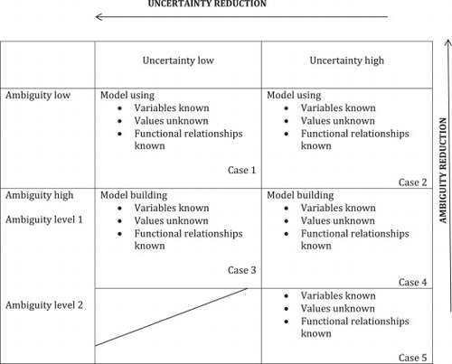
(1)	RI calculation using gauged data, either at a station on a river or spatially, without other information, has been presented in practice as an approach that is only affected by AUs. That is, the EUs are not an impediment to practice. It is possible that the denial of EUs, or at least an absence of their discussion among practicing hydrologists, was necessary to give credibility to their analyses; a syndrome known in other professions such as economics and medicine. But some research hydrologists (e.g. Dooge, 1986) vigorously challenged the epistemic underpinnings of this approach to flood forecasting, and even asked if hydrology is a science. Non-stationarity raises EU issues in particular because it shows that changes to climate and catchment characteristics need to be taken into account in flood forecasting. It therefore also raises serious issues if the AUs attached to forecasts are dependent upon a wider range of variables, many of which are poorly specified and enumerated, and the key variables in some cases unknown. For example debate continues about the role of forests in reducing or increasing flood magnitude (Calder, 1999). For many years RIs were represented as having low ambiguity and, although the uncertainties of extrapolated values of low RI were often high, they were thought to be reducible by data collection and better statistical models. Therefore as represented by practioners this approach falls into Case 1 (Fig. 1). But the EUs were always high and actually fall into Case 2. Recognition of non-stationarity has moved the field into Cases 3 and 4. The power law approach is probably an example of Case 5 because the functional relationships remain controversial and the physical causes ambiguous.
(2)	RI calculation that includes climatology certainly reduces EUs and also improves AUs, both at a river gauge and also spatially. But forecasting depends upon some view of future climate that is usually provided by a global climate model. The accuracy of a forecast is dependent upon all of the ambiguities and uncertainties listed in #1 above plus the uncertainties and ambiguities of the climate model or ensemble of climate models. This is an example of Case 2 at best and most probably Cases 3 and 4. Further, EUs are large where understanding is limited and the AUs are therefore either unknown or are large. This is a Case 4 or 5.
(3)	Calculation of MPFs and MFEs has large associated EUs because of the absence of a physical underpinning. AUs are also likely to be large because there is no confidence that the data contain the truly largest events. This is a Case 4 or 5.
(4)	Including palaeoflood and historical flood data improves AUs by extending the magnitude record to better define the upper tail of a probability density function, although the improvement is dependent upon the length of both the gauged record and the palaeoflood and historical record among other variables. The uncertainties attached to estimates of the age of events unrecorded at gauges mostly increases AUs. This addition to the calculation of RIs may move the analysis from Case 2 to Case 1 in the best examples, but this depends upon the reliability of the functional relationships that, as seen already, are not well specified. The inclusion of palaeoflood and historical data in power law analyses has much promise but remains an example of Case 5 until this approach receives more attention.

4 Organizational response, scenarios, and adaptive forecasting

According to Schrader et al. (1993) if uncertainty is considered alone, problem solving will produce results similar to those produced in the past, hopefully with lower uncertainties. Organizations charged with making flood forecasts may for example include climate state and palaeofloods in probabilistic forecasts. That is, they will use established pathways (but new information) to reduce uncertainty rather than find new pathways to reduce ambiguity. If however ambiguities are allowed an organization will search for ways of reducing them and outcomes will be different from those of the past. In flood forecasting obvious ambiguities are: whether or not to use frequentist or Bayesian statistics; and the identification of the appropriate probability distribution and its physical underpinnings.

In the first case of ambiguity, which assumes that a probabilistic approach is to be pursued, a Bayesian analysis may enable formal updating and improvement of the probabilistic input to policy, adding to the injunctions of Swanson et al. (2010). This approach could be called ‘adaptive forecasting’. This statistical approach can deal with all kinds of randomness, non-randomness, and both quantitative and qualitative information (Clegg, 2013). To use this approach an initial estimate of the probability of a large flood is made based on whatever information is available and then the estimate is improved with later information. Bayes’ theorem is:

The probability of A, given B, is equal to the probability of B given A times the probability of A, divided by the probability of B. In the case of the Ping River A could be an enormous flood and B is the joint probability of a saturated catchment and a typhoon. Using gauged, historical and palaeoflood data, and documented typhoons it should be possible to produce a ‘prior’, that is a first best estimate of the probability of A. If in the future it becomes possible to estimate the incidence of typhoons coming from the South China Sea based on sedimentary records (analogous to flood sedimentary records), the ‘prior’ can be converted into a ‘posterior’, that is the next best estimate of A. This approach can also be used in the decision-making process to which flood analysis is an input. Silver (2012) makes a strong case for a change of attitude to prediction where a Bayesian approach replaces the frequentist approach. And given that the Bayesian approach can include qualitative information, the input of historians could be crucial. Compilations of the kind by Mauch and Pfister (2009) include information relevant to flood forecasting as well as histories of vulnerability trajectories and their causes.

In the second and more profound case of ambiguity in flood forecasting, namely the appropriate probability distribution and its physical underpinnings, if it could be shown that power law distributions of say peak flood discharges are poised in the critical state between two phases (disorder and order) (Buchanan, 2000; Sornette, 2001), then a physical basis has been found for the universal use of fractal distributions and ambiguity reduced possibly to zero. However there will still be uncertainty, as all of the data used to construct a fractal distribution will have errors, and the length of record will always limit extrapolated estimates of very low AEPs. Also ambiguity may continue to exist as science finds new ways to explain the patterns in nature. That is, the problem is likely to change, along with the solutions. There is no objectively defined problem definition of the kind preferred by the standards approach of engineers (Sayers et al., 2013).

If an organization charged with flood risk management chooses to ignore ambiguity in flood forecasting, perhaps because of a lack of resources, and/or expertise, then uncertainty will remain high. Case 1 in the Matrix is the only one where certainty prevails and a single unchanging forecasting method is possible. In very rare circumstances flood forecasting is in Case 1, but this is optimistic and certainly will not persist as climate changes. Almost all examples of flood forecasting are in Cases 2, 3, 4 and even 5 depending in part upon the stage of development of the science. But this is a dynamic field of research and practice, and as EUs decline so approaches can move between the Matrix Cases. New ideas begin in Case 5 and move into Cases with less ambiguity and uncertainty. Firestein (2012) (p. 28) evocatively describes a process by which science produces ideas that begin in Case 5: ‘Science (and I think this applies to all kinds of research and scholarship) produces ignorance, possibly at a faster rate than it produces knowledge’.

It is not expected by this author that ambiguity in flood forecasting will be dramatically reduced in the near future. Following Firestein a lot of ignorance has been created by the introduction into the debate of climate state, palaeofloods, Bayesian statistics, and power laws, but a successor to the traditional engineering-based standards approach, of probabilistic forecasts based on gauged data and the adoption of design RIs and use of PMFs, is not yet available.

However, in the interests of making progress in the design of better forecasting methods, adaptive methods are needed. Perhaps the most telling comment on this matter is that by Walker, Haasnoot, and Kwakkel (2013) (p. 972) when they conclude: “‘Monitor and adapt’ is gradually becoming preferred to ‘predict and act”’. While these comments were directed at monitoring the physical system and acting to mitigate flood effects by reducing vulnerability, the comments apply equally to the development of more adaptive flood forecasting methods. Milly et al. (2008) recommend the maintenance of a robust monitoring system, which can be used to update hydrologic records and models; particularly stochastic models. But Pielke (2009) sees little value in attempting to make forecasts. He suggests the provision of a range of plausible futures (scenarios) for adaptive policy making that will require inputs from all the science and knowledge discussed here and not just a limited component. At the extreme these scenarios might include low probability-high consequence events known also as ‘worst cases’ (Clarke, 2008) or ‘pear-shaped’ phenomena (Aon Benfield, 2013) the identification of which requires histories based on information sources other than but including measured flows.

With regard to adaptive policy design for flood forecasting this author can do no better than to repeat the injunctions of Swanson et al. (2010): (1) use integrated and forward-looking analysis; (2) monitor key performance indicators to trigger built-in policy adjustments; (3) undertake formal policy review and continuous learning; (4) use multi-stakeholder deliberation; (5) enable self-organization and social networking; (6) decentralize decision-making to the lowest and most effective jurisdictional level; and (7) promote variation in policy responses. For long-term flood forecasting: #1 invites the use of all possible information about the flood system and be open to both probabilistic forecasting and scenario analysis; #2 requires a clear view of the methods to be used to reduce uncertainty and ambiguity with indicators of progress, but will only be possible where an organization can allow new pathways of thought and action or can change to achieve such pathways; #3 is clearly essential but will require organizational support and resourcing; #4 requires consultation of people likely to be affected by flood forecasts; #5 is critical to enable hydrologists, engineers, historians, archivists, and local people with historical awareness to derive flood forecasts that meet the needs of #1; #6 this will enable the interaction of ‘experts’ with local people who can enrich and broaden understanding of flood histories and risks; and #7 is consistent with the idea that there is no immutable and objective problem definition (Schrader et al., 1993).

As already seen, there are cogent reasons for not attempting to make forecasts of extreme events and poor forecasts may produce a false sense of certainty, as argued by Benson (1973) in the case of engineering design. Anderson (2000) notes that ‘…experiential information coupled with understanding can be more useful than uncertain predictions’, an approach that for example has been applied to engineering design based on the maximum likely level of earthquake stress derived from historical records and understanding of the phenomenon, an approach analogous to the identification of ‘worst case’ floods from historical records and that could be extended to include local knowledge. Acceptable probabilities based on historical records can also be used, an argument for the inclusion of historians in the analysis.

It is however hard to imagine progress in flood risk management without estimates of extreme flood magnitudes and frequencies, particularly for the construction of critical infrastructure (e.g. large dams) that can cause major damage if failure occurs. The future of flood forecasting therefore lies in striving for best estimates using a larger arsenal of tools than has been traditionally used. This calls for a deeply cross-disciplinary effort for research and practice, and the adoption of adaptive forecasting to cope with the effects of climate change.

5 Conclusions

Quantitative probabilistic long-term flood forecasts are a central feature of flood risk management despite serious associated uncertainty and ambiguity as illustrated here by using the Uncertainty-Ambiguity Matrix of Schrader et al. (1993). This unsatisfactory situation is likely to worsen as climate changes and floods become larger and possibly more frequent. Despite trenchant criticisms by a few research hydrologists and geologists/geomorphologists, quantitative probabilistic long-term flood forecasting remains the major scientific input to infrastructure design, flood-prone land zoning and evacuation planning. Stochastic models are claimed to be the answer to the problem of non-stationarity both in the present and the future as climate changes. But these models will be limited by short gauged records that usually do not capture extremes and therefore are an insufficient basis for even the most sophisticated mathematics.

Considerable progress has been made in introducing new approaches to flood forecasting, including: analysis of flood records by decomposing them according to causal climate states; extending gauged records by using palaeoflood and other non-gauged flood reconstructions; and scenario analyses particularly of ‘worst cases’ that are likely to be identified using documentary and geologic/geomorphic archives. These additions to the toolbox of flood forecasters have yet to receive widespread endorsement by organizations making flood forecasts, and will require additional research to increase their reliability. In addition, such organizations may need to change their ways of operating, personnel, and resourcing if these new ideas for reducing uncertainty are to be embraced.

But there is an additional and more profound issue: the ambiguity produced by a lack of theory underpinning flood forecasting. Progress has been made, and the existence of scale-free distributions may be a sign that a theory is possible, but there is no agreed theoretical basis for the choice of a probability density function for forecasting which means that floods are not well understood.

Progress has been made in broadening the information base of forecasting, but more is needed, and the input of many disciplines is clearly a high priority, in particular from historians and earth scientists. However, climate change presents a particular challenge that will demand greater flexibility in organizations making forecasts. Possible ways forward are to enhance monitoring (the opposite of what has been happening in many countries), to enable the updating of records coupled to non-traditional reconstructions of flood series and hydrologic models, identify plausible scenarios for policy design, and use Bayesian statistics to formally update forecasts based on all available information.

While some scholars question the practicality and even the advisability of forecasting, it is unlikely to stop. The approach recommended here is for ‘adaptive forecasting’ by flexible and agile organizations and people.

Acknowledgements

Thanks are extended to the organizers of the International Conference on Uncertainty and Policy Design 27–28 November 2014 Chengdu, China where this paper was first presented. The Institute of Water Policy at the Lee Kuan Yew School of Public Policy, National University of Singapore, provided funding. Two anonymous reviewers helped to improve the paper.

References

- T.L. Anderson . Design of critical facilities without time-specific predictions. D. Sarawitz , R.A. Pielke Jr. , R. Byerly . Prediction: Science, decision making, and the future of nature. 2000; Island Press: Washington, DC, 364–365.
- Aon. Benfield . Pear-shaped phenomena: Low probability, high consequence events. 2013
- V.R. Baker . Paleoflood hydrology: Origin, progress, prospects. Geomorphology. 101: 2008; 1–13.
- D.N. Barnett , J. Simon , J.M. Brown , D.M.H. Murphy , H. Sexton , M.J. Webb . Quantifying uncertainty in changes in extreme event frequency in response to doubled CO2 using a large ensemble of GCM simulations. Climate Dynamics. 26: 2006; 489–511.
- M.A. Benson . Thoughts on the design of design floods, in floods and droughts. Proceedings of the 2nd International Symposium in Hydrology. 1973; Water Resources Publication: Fort Collins, Colorado, 27–33.
- D. Bewsher , J. Maddocks . Do we need to consider floods rarer than 1% AEP?. Horsham 2003 – HEALTHY Floodplains WEALTHY Future. 2003. 6 pp. (http://www.bewsher.com.au/pdf/CNF40P_1.pdf).
- M. Buchanan . Ubiquity: The science of history or why the world is simpler than we think. 2000; Weidenfeld and Nicholson: London, 230 pp..
- I.R. Calder . The blue revolution: Land use and integrated water resources management. 1999; Earthscan: London, 192 pp..
- A. CapotondI , E. Guilyardi , B. Kirtman . Challenges in understanding and modeling ENSO. PAGES Newsletter. 2013(2): 2013; 58–59. (http://www.pages-igbp.org/download/docs/newsletter/2013-2/Full_references.pdf).
- L. Clarke . Thinking about worst-case thinking. Sociological Inquiry. 78: 2008; 154–161.
- B. Clegg . Dice World: Science and life in a random universe. 2013; Icon: London, 274 pp..
- M. Collins , S.-I. An , W. Cai , A. Ganachaud , E. Guilyardi , F.-F. Jin , M. Markus Jochum , M. Lengaigne , S. Power , A. Timmermann , G. Vecchi , A. Wittenberg . The impact of global warming on the tropical Pacific Ocean and El Niño. Nature Geoscience. 3: 2010; 391–397.
- Dawdy . Prediction versus understanding (The Ven Te Chow Lecture). Journal of Hydrologic Engineering. 2007, January/February; 1–3.
- M.N. Desa , P.R. Rakhecha . Probable maximum precipitation for 24-h duration over an equatorial region: Part 2-Johor, Malaysia. Atmospheric Research. 84: 2007; 84–90.
- J.C.I. Dooge . Looking for hydrologic laws. Water Resources Research. 22(9): 1986; 46S–58S.
- E.M. Douglas , A.P. Barros . Probable maximum precipitation using multifractals: Application in the Eastern United States. Journal of Hydrometeorology. 4: 2003; 1012–1024.
- D.A. Eash , K.K. Barnes , A.G. Veilleux . Methods for Estimating Annual Exceedance-Probability Discharges for Streams in Iowa, Based on Data though Water Year 2010. USGS Scientific Investigations Report 2013-5086. 2013
- S. Firestein . Ignorance: How it drives science. 2012; Oxford University Press. 195 pp..
- F. Francés , B.A. Botero . Probable maximum flood estimation using systematic and non-systematic information. V.R. Thorndycraft , G. Benito , M. Barriendos , M.C. Llasat . Palaeofloods, historical floods and climatic variability: Applications in flood risk assessment (Proceedings of the PHEFRA Workshop, Barcelona, 16, 2002). 2003
- F. Francés , J.D. Salas , D.C. Boes . Flood frequency analysis with systematic and historical or palaeoflood data based on the two-parameter general extreme value models. Water Resources Research. 30(6): 1994; 1653–1664.
- W.E. Fuller . Flood flows. Transactions of the American Society of Civil Engineers. 68: 1914; 564–618.
- W.J. Graham . Should dams be modified for the probable maximum flood?. Journal of the American Water Resources Association. 36(5): 2000; 953–963.
- V.K. Gupta , B.M. Troutman , D.R. Dawdy . Towards a nonlinear geophysical theory of floods in river networks: An overview of 20 years of progress. A.A. Tsonis , J.B. Elsner . Nonlinear dynamics in geosciences. 2007; Springer. 121.-151.
- C. Hood , H. Rothstein , R. Baldwin . The Government of risk-understanding risk regulation regimes. 2004; Oxford University Press: Oxford, 232 pp..
- D. Jakob , R. Smalley , J. Meighen , K. Xuereb , B. Taylor . Climate change and probable maximum precipitation. 2009; Bureau of Meteorology, Australian Government, Hydrometeorological Advisory Service, Water Division: Melbourne, (www.bom.gov.au/hydro/has/).
- V. Kale , V. Baker . An extraordinary period of low-magnitude floods coinciding with the Little Ice Age: Palaeoflood evidence from Central and Western India. Journal of the Geological Society of India. 68: 2006; 477–483.
- A.S. Kiem , S.W. Franks , G. Kuczera . Multi-decadal variability of flood risk. Geophysical Research Letters. 30(2): 2003; 1035. 10.1029/2002GL015992. 7 pp..
- F.H. Knight . Risk, uncertainty, and profit. 1921; Hart, Schaffner & Marx; Houghton Mifflin Company: Boston, MA
- D. Koutsoyiannis . A probabilistic view of Hershfield's method for estimating probable maximum precipitation. Water Resources Research. 35(4): 1999; 1313–1322.
- H.D. Lasswell . The emerging conception of the policy sciences. Policy Sciences. 1: 1970; 3–14.
- B. Malamud , D. Petley . Lost in translation. Science and Technology. 02: 2009; 164–167. (http://www.kcl.ac.uk/sspp/departments/geography/people/academic/malamud/lostintranslation.pdf).
- B.D. Malamud , D.L. Turcotte . The applicability of power-law frequency statistics to floods. Journal of Hydrology. 322: 2006; 168–180.
- C. Mauch , C. Pfister . Natural disasters, cultural responses. 2009; Lexington Books: Plymouth, 382 pp..
- N. Millington , S. Das , S.P. Simonovic . The comparison of GEV, Log Pearson Type 3 and Gumbel distributions in the upper Thames River Watershed under global climate models. 2011; Department of Civil and Environmental Engineering, The University of Western Ontario, London: Ontario, Canada
- P.C.D. Milly , J. Betancourt , M. Falkenmark , R.M. Hirsch , Z.W. Kundzewicz , D.P. Lettenmaier , R.J. Stouffer . Stationarity is dead: Whither water management?. Science. 319: 2008; 573–574.
- G.C. Nanson , J.C. Croke . A genetic classification of floodplains. Geomorphology. 4: 1992; 459–486.
- S. Nobert , K. Krieger , F. Pappenberger . understanding the roles of modernity, science, and risk in shaping flood management. Natural Hazards and Earth System Science. 14: 2015; 1921–1942.
- B.D. Phillips , M. Fordham . Introduction. B.D. Phillips , D.S.K. Thomas , A. Fothergiill , L. Blinn-Pike . Social vulnerability to disasters. 2010; CRC Press: Boca Raton, 392 pp..
- B.D. Phillips , D.S.K. Thomas , A. Fothergiill , L. Blinn-Pike . Social vulnerability to disasters. 2010; CRC Press: Boca Raton, 392 pp..
- R. Pielke Jr. . Collateral damage from the death of stationarity. GEWEX, WRCP. 2009; 5–7. (http://sciencepolicy.colorado.edu/admin/publication_files/resource-2725-2009.11.pdf).
- O.H. Pilkey , L. Pilkey-Jarvis . Useless arithmetic: Why environmental scientists can’t predict the future. 2007; Columbia University Press: New York, 230 pp..
- Plate . Flood risk and flood management. Journal of Hydrology. 267: 2002; 2–11.
- D. Sarewitz , R.A. Pielke Jr. . Prediction in science and policy. D. Sarawitz , R.A. Pielke Jr. , R. Byerly . Prediction: Science, decision making, and the future of nature. 2000; Island Press: Washington, DC, 11–22.
- P. Sayers , Y. Li , G. Galloway , E. Penning-Rowsell , S. Fuxin , W. Kang , C. Yiwei , T.L.E. Quesne . Flood risk management: A strategic approach. 2013; Asia Development Bank. 202 pp..
- A.E. Scheidegger . Physical aspects of natural catastrophes. 1975; Elsevier: Amsterdam, 289 pp..
- S. Schrader , W.M. Riggs , P. Robert , R.P. Smith . Choice over uncertainty and ambiguity in technical problem solving. Journal of Engineering and Technology Management. 10: 1993; 73–99.
- N. Silver . The signal and the noise: The art and science of prediction. 2012; Penguin: London, 534 pp..
- D. Sornette . Critical phenomena in natural sciences. 2001; Springer: New York
- D. Swanson , S. Barg , S. Tyler , H. Venema , S. Sanjay Tomar , S. Bhadwal , S. Nair , D. Roy , J. Drexhage . Seven tools for creating adaptive policies. Technological Forecasting & Social Change. 77: 2010; 924–939.
- N.N. Taleb . Antifragile: Things that gain from disorder. 2013; Penguin. 519 pp..
- USGS (United States Geological Survey) . 100-year flood-it's all about chance. Haven’t we already had one this century?. General Information Product. 2010; 106.
- D.C. Verdon , S.W. Franks . Long-term behaviour of ENSO: Interactions with the PDO over the past 400 years inferred from paleoclimate records. Geophysical Research Letters. 33: 2006; L06712. 10.1029/2005GL025052. 5 pp..
- R.M. Vogel , N.C. Matalas , J.F. England Jr. , A. Castellarin . An assessment of exceedance probabilities of envelope curve. Water Resources Research. 43: 2007; W07403. 10.1029/2006WR005586.
- W.E. Walker , M. Haasnoot , J.H. Kwakkel . Adapt or perish: A review of planning approaches for adaptation under deep uncertainty. Sustainability. 5: 2013; 955–979.
- R.J. Wasson , Y.P. Sundriyal , S. Chaudhary , M.K. Jaiswal , P. Morthekai , S.P. Sati , N. Juyal . A 1000-year history of large floods in the Upper Ganga catchment, central Himalaya, India. Quaternary Science Reviews. 77: 2013; 156–166.
- B. Wisner , P. Blaikie , T. Cannon , I. Davis . At risk: Natural hazards, people's vulnerability and disasters. 2004; Routledge: London, 471 pp..
- WMO (World Meteorological Organisation) . Manual of extreme probable maximum precipitation. WMO-No. 1045. 1986. 257 pp..
- G. Woo . Calculating catastrophe. 2011; Imperial College Press: London, 355 pp..