Minimizing total completion time on a single machine with step improving jobs

Abstract

Production systems often experience a shock or a technological change, resulting in performance improvement. In such settings, job processing times become shorter if jobs start processing at, or after, a common critical date. This paper considers a single machine scheduling problem with step-improving processing times, where the effects are job-dependent. The objective is to minimize the total completion time. We show that the problem is NP-hard in general and discuss several special cases which can be solved in polynomial time. We formulate a Mixed Integer Programming model and develop an LP-based heuristic for the general problem. Finally, computational experiments show that the proposed heuristic yields very effective and efficient solutions.

Keywords:

• scheduling
• step-improving processing times
• total completion time
• heuristic

after four revisions

The online version of this article is available Open Access

1. Introduction

Most classical scheduling models assume that job processing times remain constant over time. However, in various real-life production and manufacturing systems job processing times change over time. The contributing factors to varying processing times may be machine or worker learning, machine deterioration, production system upgrades or technological shocks. Gawienjnowiz (2008) provides a wide variety of applications and to date results on scheduling with time-dependent jobs. Time-dependent scheduling models can be classified into three general categories. The first category consists of linear models, whereby job processing times increase or decrease linearly as a function of the job’s start time. The first papers to introduce time deteriorating jobs were Gupta et al (1987), Gupta and Gupta (1998), and Browne and Yechiali (1990). The authors of these papers assumed that job processing times consist of two components. The former is a basic processing time which remains constant throughout the planning horizon. The latter varies over time and is the product of the job start time and a job-dependent deterioration index. The makespan minimization problem on a single machine is shown to be solved in polynomial time using a simple sorting rule; however, the total completion time counterpart remains open even when the basic processing times are assumed to be identical for all jobs (see Mosheiov, 1991). The second category of time-dependent processing time scheduling models addresses piece-wise linear job processing time functions. The underlying assumption of these models is that job processing times remain constant until a certain event occurs. Following changes in the production setting, job processing times begin to increase, or in some cases decrease, linearly at a predefined point in time. Cheng et al (2004) and the references within describe a variety of applications for this class of models, including fire fighting efforts, searching for items under worsening light or weather conditions and maintenance scheduling. Wu et al (2009) propose a branch-and-bound algorithm as well as heuristic algorithms for solving a single machine scheduling problem with the objective of minimizing the makespan. Farahani and Hosseini (2013) show that a single machine scheduling problem with the objective of minimizing the cycle time where the job processing time is a piecewise linear function of its start time is polynomially solvable. The third category is devoted to scheduling settings where job processing times have two possible values, depending on their start time. The motivation for such models arises from systems which experience a single discrete change in setting. For example, the introduction of a new technology or the purchase of a more efficient machine. Under this model job processing times do not change over time and are only affected by the different machine setting. These models are often referred to as step-deteriorating or step-improving problems, depending on the context. Step-deteriorating models were first introduced by Sundararaghavan and Kunnathur (1994) and later studied by Mosheiov (1995), Cheng and Ding (2001) and Jeng and Lin (2004). The makespan minimization problem was shown to be NP-hard in the ordinary sense by both Mosheiov (1995) and Cheng and Ding (2001). The same problem under the assumption that each job has a distinct event which affects its processing time is also NP-hard (see Jeng and Lin, 2004). Cheng and Ding (2001) also addressed the total completion time objective, showing that the problem is strongly NP-hard. In a recent paper, Cheng et al (2006) study a makespan minimization problem with step-improving processing times and a common critical date. They prove the problem is NP-hard and develop an efficient pseudo-polynomial time algorithm. They also introduce a Fully Polynomial Time Approximation Scheme (FPTAS) and an online algorithm with a worst case ratio of 2. Ji et al (2007) address the same problem and develop a simple linear time algorithm with a worst case ratio of 5/4. For earlier results on scheduling with step-improving or step-deteriorating processing times, we refer the reader to two extensive survey papers by Alidaee and Womer (1999) and Cheng et al (2004).

Recently, some studies investigate time-dependent scheduling models with other variations of classic scheduling models. Cai et al (2011) consider the single machine scheduling problem with time-dependent processing times and machine breakdowns. The objectives are to minimize the expected makespan and the variance of the makespan. Mor and Mosheiov (2012) consider a classical batch scheduling model with step-deterioration of processing times. The objective is to minimize flowtime. Qian and Steiner (2013) consider a single machine scheduling problem with learning/deterioration effects and time-dependent processing times. By using special assignment problem on product matrices, they solve the problem in near-linear time. Lu et al (2014) consider a single machine scheduling problem with decreasing time-dependent processing times and group technology assumption. The group setup times and job processing times are both decreasing linear functions of their starting times. They show that the problem can be solved in polynomial time.

In this paper we consider the same setting as Cheng et al (2006) and Ji et al (2007): we assume a single machine scheduling environment and a common critical date after which job processing times reduce by a job-dependent amount. To the best of our knowledge, this is the first paper to consider a single machine setting with step-improving jobs and a critical date under a scheduling criterion which is not the makespan. We consider the total completion time objective which is paramount in determining the work in process of a manufacturing system and the level of service provided to customers. The focus on a min-sum type objective gives rise to interesting problem characteristics, various special cases which can be solved optimally and a very efficient approximation scheme for the general setting. We begin by introducing some notation in Section 2. We show that the total completion time minimization problem is NP-hard in Section 3, and discuss several special cases which can be solved in polynomial time in Section 4. We formulate a Mixed Integer Programming (MIP) model and develop an LP-based heuristic for the problem in Section 5. In Section 6, computational experiments are performed. Some concluding remarks and directions for future research are given in Section 7.

2. Problem description

A set of n non-preemptive jobs N={1, …, n} is available for processing at time zero. All jobs in N share a common critical date D which affects their processing times. The processing time of job j is specified by two integers a_j and b_j with 0⩽b_j⩽a_j. If job j begins processing at some time t<D, then its processing time equals a_j; if it starts at some time t⩾D, then its processing time is a_j−b_j. The goal consists of finding a non-preemptive schedule which minimizes the total completion time.

A schedule σ is an assignment of the jobs in N to the single machine such that each job receives an appropriate amount of processing time, and no two jobs can be processed on the single machine at the same time. Let S_j(σ) and C_j(σ) denote the start and finish times of job j in schedule σ, respectively. We represent S_j(σ) as S_j and C_j(σ) as C_j when schedule σ is clear from the context. Let σ* represent the optimal schedule, that is, the one which minimizes the total completion time, and let ∑C_j(σ*) denote the minimum total completion time associated with this schedule. Let [i] denote the job in the ith position of the job sequence.

The standard classification scheme for scheduling problems (Graham et al, 1979) is α₁|α₂|α₃, where α₁ describes the machine structure, α₂ gives the job characteristics or restrictive requirements, and α₃ defines the objective function to be minimized. We extend this scheme to provide for the step-improving processing time with a common critical date by using p_j=a_j or p_j=a_j−b_j and d_j=D in the α₂ field. Our problem can be denoted as 1|p_j=a_j or p_j=a_j−b_j, d_j=D|∑C_j.

3. Complexity results

This section studies the complexity issue of the considered problem. A reduction method is used from the following problem, which is known to be NP-complete.

Even-odd partition (Garey and Johnson, 1979): Given positive integers x₁, x₂, …, x_2t, where x₁⩽x₂⩽⋯⩽x_2t, does it exist a set X⊆T={1, 2, …, 2t} such that ∑_j∈Xx_j=∑_j∈T\Xx_j=r, and X contains exactly one of {x_2j−1, x_2j} for j=1, 2, …, t? Assume without loss of generality that r>3t. If not, then we can multiply each partition element and partition size by 3t without changing the solution of the problem.

Given any instance of even-odd partition problem with t, r and x_j for j=1, …, 2t, we consider the following instance of 1|p_j=a_j or p_j=a_j−b_j, d_j=D|∑C_j, called instance I:

A threshold value, K, is defined as K=Σ_j=1^t(t−j+1)(x_2j−1+x_2j)+(3t²+3t)r²+(t+4)r. In the following we prove that there exists a schedule for this instance of 1|p_j=a_j or p_j=a_j−b_j, d_j=D|∑C_j with ∑C_j⩽K if and only if there exists a solution to even-odd partition problem.

Lemma 1

• If there exists a solution to even-odd partition problem, there exists a feasible schedule for instance I.

Proof

• Since there exists a solution to even-odd partition, the elements are reindexed such that Σ_j=1^tx_2j−1=Σ_j=1^tx_2j=r. Consider a schedule σ as constructed in Figure 1. The jobs 2j−1 for j=1, …, t are scheduled in this order without idle time. Then, since Σ_j=1^ta_2j−1=D, jobs 2j for j=1, …, t and job 2t+1 are scheduled in this order starting at time D without idle time. Thus,

  Figure 1 The structure of schedule σ.

  

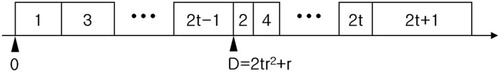
  The third equality follows because Σ_j=1^t(a_2j−b_2j)=r. This implies that there exists a feasible schedule with ∑C_j⩽K for instance I. □

We now show that a feasible solution to instance I implies a solution to even-odd partition. Let σ* denote a optimal schedule for instance I.

Lemma 2

• In σ*, job 2t+1 is the last job to be processed.

Proof

• Suppose that job 2t+1 starts processing before D in σ*. Since a_2t+1=2r²+2r>2r²+x_j=a_j for j=1, …, 2t, job 2t+1 and the last job for processing, job [2t+1], can be interchanged while the total completion time decreases or remains the same, where job [i] denotes the job in the ith position in a given sequence. Alternatively, suppose that job 2t+1 starts processing after D in σ*. For the jobs starting after D, the SPT (Shortest Processing Time) rule is optimal (Smith, 1956). Therefore, job 2t+1 must be the last job in σ* because a_2t+1−b_2t+1=2r>x_j=a_j−b_j for j=1, …, 2t. □

Lemma 3

• In σ*, there are exactly t jobs that start processing before D, and the total processing time of these jobs is not greater than D.

Proof

• Observe that a_j>2r² for j=1, …, 2t and 2r²t<D<2r²(t+1). Thus, there are at most t+1 jobs that start processing before D. Suppose that t+1 jobs start processing before D. Then, it follows that C_[t+1]>2r²(t+1). Since 2r²(t+1)>D+(a_[t+1]−b_[t+1]), the total completion time can be decreased by inserting idle time so that job [t+1] start processing at D. Consequently, exactly t jobs start processing before D in σ*.

  Furthermore, the total processing time of the first t jobs is not greater than D. Otherwise, since Σ_j=1^2t(a_j−b_j)=2r, it follows that Σ_j=t+1^2ta_[j]<D. Therefore, for j=1, …, t, job [j] and job [t+j] can be interchanged while the total completion time decreases or remains the same. □

Theorem 1

• The problem 1|p_j=a_j or p_j=a_j−b_j, d_j=D|∑C_jis NP-hard even when b_j=b for all j.

Proof

• Lemma 1 shows that a solution to even-odd partition implies a feasible schedule for instance I. To complete the proof, we must now show that a feasible schedule for instance I implies a solution to even-odd partition.

  From the results of Lemma 2 and Lemma 3, exactly t jobs in {1, …, 2t} start processing before D, and t jobs in {1, …, 2t} and job 2t+1 start processing from D. Thus, similar to the analysis in Lemma 1, the total completion time can be expressed as

  The third equality follows from the fact that Σ_j=1^t(a_[t+j]−b_[t+j])=Σ_j=1^tx_[t+j]=2r−Σ_j=1^tx_[j].

  Since Σ_j=1^2t+1C_j⩽K and Σ_j=1^tx_[j]⩽r, it follows that {x_[j], x_[t+j]}={x_2j−1, x_2j} for j=1, …, t and Σ_j=1^tx_[j]=r. As a result, the set of jobs that start processing before D provides a solution to even-odd partition problem, which indicates that a feasible schedule for instance I implies a solution to even-odd partition.

  By combining Lemma 1 and the proof above, there exists a schedule for this instance of 1|p_j=a_j or p_j=a_j−b_j, d_j=D|∑C_j with ∑C_j⩽K if and only if there exists a solution to even-odd partition problem. Therefore, the problem 1|p_j=a_j or p_j=a_j−b_j, d_j=D|∑C_j is NP-hard even when b_j=b for all j. □

4. Polynomially solvable cases

In this section, we study several special cases of the problem which can be solved in polynomial time.

4.1. All processing times improve according to a fixed ratio b_j=δa_j for all 1⩽j⩽n, and there exists k such that Σ_j=1^ka_j=D

We first focus on the case where jobs are shortened according to a fixed ratio if they start processing at, or after, the common critical date D. If there exists k such that Σ_j=1^ka_j=D, then we show that a simple sorting procedure yields an optimal solution for the problem. Otherwise, the problem remains NP-hard.

Lemma 4

• Suppose that a₁⩽a₂⩽…⩽a_nand b_j=δa_jfor ∀j where 0<δ<1. If there exists k such that Σ_j=1^ka_j=D, then the SPT rule with respect to a_jis optimal.

Proof

• For a given schedule, there are two sets of jobs: jobs that start processing before D and jobs that start processing after D. Since the SPT rule on each set of jobs is optimal, it suffices to show that jobs in {1, …, k} are scheduled in the time interval [0, D] in an optimal schedule.

  Consider a schedule σ where some jobs in {k+1, …, n} start processing before D. In σ, let A denote a set of jobs that start processing before D, let B denote a set of jobs that start processing after D. Let X=A∩{k+1, …, n} and Y=B∩{1, …, k}. Note that the SPT rule on each set of jobs is optimal. Thus, since a_i⩽a_j for i∈A\X and j∈X, jobs in X do not precede any jobs in A\X. Similarly, since a_i−b_i=(1−δ)a_i⩽(1−δ)a_j=a_j−b_j for i∈Y and j∈B\Y, jobs in Y have to precede jobs in B\Y. Let x_[i] and y_[i] denote the jobs in the ith position of the job sequences in X and Y, respectively. Figure 2 depicts the schedule σ.

  Figure 2 Two possible structures of schedule σ.

  

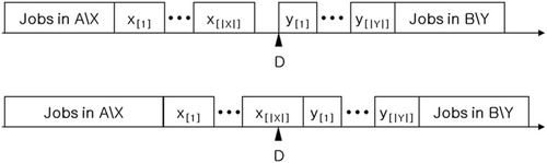
  We first show that |X|⩽|Y|. Suppose that |X|>|Y|. From the assumption that a₁⩽a₂⩽…⩽a_n, we obtain that for i=1, …, |Y|. Therefore, we can exchange x_[i] and y_[i] for i=1, …, |Y| without increasing the start time of x_[|Y|+1]. This implies that k+1 jobs can start its processing before D, which contradicts to the assumption that Σ_j=1^ka_j=D, that is, at most k jobs can start it processing before D. Alternatively, we assume that |X|⩽|Y|.

  As shown in Figure 2, there are two cases: ∑_j∈Aa_j<D and ∑_j∈Aa_j⩾D.

  Case 1:

  =

  ∑j∈Aaj<D.

  Since ∑_j∈Aa_j<D, observe that

  Construct a new schedule σ′ by interchanging jobs in A and jobs in B in the same order as in σ. Let t=D−∑_j∈A\Xa_j. Then,

  Since |X|⩽|Y|,

  The last inequality follows because for i=1…|X|, and δ∑_j∈Ya_j<t and ∑_j∈Xa_j<∑_j∈Ya_j. As a result, we can create a new schedule σ′ where jobs in {1, …, k} are scheduled in the time interval [0, D] without increasing the total completion time.

  Case 2:

  =

  ∑j∈Aaj⩾D.

  Since ∑_j∈Aa_j⩾D, we obtain

  Let s=∑_j∈Xa_j and t=D−∑_j∈A\Xa_j, respectively. Observe that s⩾t. Construct a new schedule σ′ by interchanging jobs in A and jobs in B in the same order as in σ. Then,

  Since |X|⩽|Y|,

  The last inequality follows because t⩽s, and for i=1…|X|, and δ∑_j∈Ya_j<s and ∑_j∈Ya_j⩾∑_j∈Xa_j. As a result, we can create a new schedule σ′ where jobs in {1, …, k} are scheduled in the time interval [0, D] without increasing the total completion time. □

In the following we present an example to demonstrate that even when a₁⩽a₂⩽…⩽a_n and b_j=δa_j for ∀j where 0<δ<1, if there does not exist any k such that Σ_j=1^ka_j=D, then the SPT rule may not be optimal. Consider an example where there are three jobs with a₁=16, a₂=18 and a₃=22 while D=20 and δ=0.5. Therefore, a_j−b_j are 8, 9 and 11, respectively, for j=1, 2, 3. The SPT rule yields a solution value of 95 (the completion times are 16, 34 and 45, respectively). If we schedule job 2 first and insert an idle time of 2 time units, followed by jobs 1 and 3, then the total completion time is 85 (with completion times of 18, 28 and 39). Clearly, since at most one job can start processing before the critical date, it is beneficial to sequence the longest job which does not exceed the critical date D, that is, job 2 in our case.

4.2 All improved processing times are identical a_i−b_i=a_j−b_j for all 1⩽i,j⩽n

We consider the special case where jobs have different processing times if scheduled before D, but the same improved processing time if they start processing after D. If D does not coincide with the completion time of a job, it may be beneficial to insert some idle time before D, as shown below.

Lemma 5

• Suppose that a₁⩽a₂⩽…⩽a_nand a_i−b_i=a_j−b_jfor all 1⩽i, j⩽n. The SPT rule with respect to a_jis optimal.

Proof

• Let k denote the maximum number of jobs which can finish processing before D. Construct a schedule σ based on the SPT rule: Assign the first k jobs in non-decreasing order of a_j before D; If Σ_j=1^k+1a_j⩽D+a_k+1−b_k+1 (which is equivalent to Σ_j=1^ka_j⩽D−b_k+1), then job k+1 starts directly after job k finishes at time Σ_j=1^ka_j. If Σ_j=1^ka_j>D−b_k+1, then job k+1 starts at time D inserting idle time; The remaining jobs are assigned in non-decreasing order of a_j−b_j without any idle time.

  We now show that any feasible schedule can be changed into σ without increasing its total completion time. Take a feasible schedule σ′. Let k′ denote the number of jobs which finish processing before D in σ′. It is clear that in order to minimize the total completion time of the first k′ jobs they must be ordered according to the SPT rule with respect to a_j. The remaining jobs can be ordered arbitrarily as they have identical improved processing times. Without loss of generality we assume that the jobs processed after time D are also in SPT order. Now construct a new schedule σ″ by interchanging jobs [k′] and [k′+1], without changing the start time of the jobs [k′] and [k′+1]. From the assumption that the first k′ jobs and the latter n−k′ jobs are in SPT order, we have that . Therefore,

  By repeating this procedure, we can construct σ without increasing the total completion time for the given schedule. □

4.3. All initial processing times are identical a_j=a for all 1⩽j⩽n

Next, we consider a special case for which all jobs have the same processing time initially but different processing times if they begin processing no earlier than D. It is clear that exactly k=⌊D/a⌋ jobs can finish their processing before D. The focus is on the job [k+1] which is in the (k+1)st position in the sequence: if b_[k+1]⩽D−ka=D−⌊D/a⌋a, then job [k+1] should start at time ka; if, on the other hand, b_[k+1]⩽D−ka, then job [k+1] should start at time D.

Lemma 6

• Suppose that a_j=a for ∀j and that b₁⩾b₂⩾…⩾b_n. The SPT rule with respect to a_j−b_j(or Longest Process Time (LPT) rule with respect to b_j) is optimal.

The proof of Lemma 6 is based on a standard pair-wise interchange argument and is similar to the proof of Lemma 5. For the sake of brevity we omit the formal proof. These results are meaningful considering that the problem is NP-hard even when b_j=b, but polynomially solvable either when a_j=a or when a_i−b_i=a_j−b_j.

5. The LP-based heuristic

In this section, we develop an LP-based heuristic for the proposed problem. The scheduling problem is expressed in an MIP formulation in Section 5.1. Then, an LP-based heuristic is developed on the basis of an LP relaxation of MIP in Section 5.2.

5.1. The MIP formulation

In this section we develop an MIP formulation of the proposed problem. Without loss of generality, we assume that the jobs are indexed in non-decreasing order of a_j.

Variables

MIP:

The objective function (1) seeks to minimize the total completion time. Constraint (2) implies that the starting time of the job in the (i+1)st position in the job sequence is greater than or equal to the completion time of the job in the ith position. Constraints (3) and (4) imply that the processing time of the job in the ith position in the job sequence is a_[i] if the job starts before D and that the processing time of the job in the ith position in the job sequence is a_[i]−b_[i] if the job starts after D. Note that M is a sufficiently large number. Constraint (5) implies that a job starts either before or after D. Constraints (6) and (7) imply that exactly one job occupies exactly one position in the job sequence. Constraint (8) implies that x_ij and y_ij are binary variables. Constraint (9) implies that starting times of the jobs are nonnegative.

Lemma 7

• Constraint (3) inMIPis equivalent to

Proof

• Constraint (3) implies that ∑_j∈Nx_ij=1 if S_i<D and ∑_j∈Nx_ij=0 if S_i⩾D. Suppose that S_i<D. Since the jobs are indexed in non-decreasing order of a_j,

  Thus, 0<D−S_i<D+1−Σ_j=1ⁱ⁻¹a_j. If S_i<D, then

  which imposes ∑_j∈Nx_ij=1.

  Suppose that S_i⩾D. Then, the right-hand side of Constraint (10) is not greater than zero, which imposes ∑_j∈Nx_ij=0. As a result, Constraint (10) is equivalent to Constraint (3) in MIP. □

Observe that Constraint (10) is stronger than Constraint (3). We use Constraint (10) instead of Constraint (3) in order to reduce a search space for finding an optimal solution of MIP.

5.2. Heuristic

In this section, we develop an LP-based heuristic using the optimal solutions of an LP relaxed problem of MIP. In the LP relaxed problem of MIP, we relax the binary constraint for x_ij and y_ij, Constraint (8), and using Lemma 7, we develop the LP relaxed problem of MIP as follows.

LPR:

subject to (2), (4), (5), (6), (7), (10) and

Note that the LPR can be solved in polynomial time, using the ellipsoid method (Grotschel et al, 1993).

In the LP-based heuristic, let X and Y denote two distinct subsets of the job set N where jobs in X start processing before time D and jobs in Y start processing at, or after time D. The heuristic classifies each job into two sets, X and Y, according to an optimal solution of LPR. Then, schedule the jobs in X in non-decreasing order of a_j, and schedule the jobs in Y in non-decreasing order of a_j−b_j.

We now present a formal description of the heuristic.

The LP-based heuristic algorithm: Construction of a schedule for 1∣p_j=a_jor p_j=a_j−b_j, d_j=D∣ΣC_j.

illustration

The following example demonstrates the LP-based heuristic algorithm for a small problem containing three jobs.

Example 1

• There are three jobs with a₁=16, a₂=18, a₃=22, b₁=11, b₂=9, b₃=10 and D=20. The optimal solution of LPR can be obtained as follows:

  Since x₁₁^r+x₂₁^r+x₃₁^r<y₁₁^r+y₂₁^r+y₃₁^r, we assign job 1 in Y. Similarly, since x₁₂^r+x₂₂^r+x₃₂^r>y₁₂^r+y₂₂^r+y₃₂^r and x₁₃^r+x₂₃^r+x₃₃^r<y₁₃^r+y₂₃^r+y₃₃^r, we assign job 2 and job 3 in X and Y, respectively. Consequently, X={2} and Y={1, 3}. We schedule job 2 first, and since max{D, Σ_j∈Xa_j}=20, we schedule job 1 time 20 followed by job 3 at time 25. The heuristic yields a solution value of 80 with C₁=25, C₂=18 and C₃=37.

6. Computational study

In this section, we undertake extensive numerical tests to evaluate the quality of solutions found for problem 1∣p_j=a_j or p_j=a_j−b_j, d_j=D∣∑C_j by the proposed heuristic. The heuristic algorithm is coded in GAMS/CPLEX with the default settings, and run on a personal computer with an Intel Core i7-2600, 3.40GHZ processor. Since there is no computational study which considers the setting addressed in this paper in the existing literature, we have adapted the data generation scheme used in Jeng and Lin (2004). In Jeng and Lin (2004), the authors study a makespan minimization problem under the assumption that job processing times are a non-linear function of their start time and due-date. In order to evaluate the performance of their proposed algorithms, the authors undertake a comprehensive computational study. We have adapted their framework to our problem setting for the purpose of measuring the performance of our heuristic algorithm. In our study we aim to isolate the effects, if these exist, of the following factors: the number of jobs (n), the difference (or ratio) between the job processing times before and after the common due date (a_j and b_j), and the restrictiveness of the common due date (D). The results will allow us to determine the accuracy of the heuristic algorithm for any specific problem setting.

To test the effects of varying n and D, we let n∈{50, 100, 200, 400} and D=α∑a_j where α∈{0.2, 0.4, 0.6, 0.8}. In order to determine whether or not the range of a_j has an impact on the performance of the heuristic, we let a_j~DU[1, 50], a_j~DU[1, 100], a_j~DU[1, 150] and a_j~DU[1, 200], where DU[l, u] is the discrete uniform distribution over the interval [l, u]. Moreover, the ratio of a_j to b_j may affect the performance of the heuristic. For the associated test, we let b_j~DU[0, βa_j] where β∈{0.1, 0.4, 0.7, 1.0}.

Two sets of experiments were run. In the first set, n and D were allowed to vary, while a_j~DU[1, 100] and b_j~DU[0, a_j]. These results are presented in Table 1. In the second set, a_j and b_j were allowed to vary, while n=100 and D=0.6∑a_j. These results are presented in Table 2. Since calculating the optimal solution is computationally difficult, we use the lower bound which is the optimal solution value of the LPR as a surrogate. As a result, our performance indicator, the relative error, 100 × (z_H−z_L)/z_L, provides an upper bound for the actual sample relative error, where z_H and z_L represent the solution value of the proposed heuristic and a lower bound, respectively. For each condition, the table entry is the average of 20 instances. Times are given in seconds and only include computation time.

Table 1 Performance of the heuristic with different numbers of jobs and different common critical dates

n	D	Relative error (%)		CPU time (s)
		Average	Maximum	Average	Maximum
50	0.2∑aj	7.007	10.435	0.282	0.472
	0.4∑aj	2.883	5.186	0.293	0.360
	0.6∑aj	0.914	1.617	0.283	0.373
	0.8∑aj	0.170	0.583	0.242	0.310
100	0.2∑aj	7.513	11.056	1.297	1.562
	0.4∑aj	3.030	3.970	1.502	1.739
	0.6∑aj	0.989	1.867	1.628	2.027
	0.8∑aj	0.239	0.423	1.463	2.055
200	0.2∑aj	7.750	9.053	11.244	15.821
	0.4∑aj	3.288	4.246	14.470	19.108
	0.6∑aj	1.135	1.731	15.572	23.680
	0.8∑aj	0.172	0.312	15.564	25.148
400	0.2∑aj	7.678	8.346	179.707	272.347
	0.4∑aj	3.459	3.874	208.010	282.703
	0.6∑aj	1.184	1.534	218.957	311.451
	0.8∑aj	0.188	0.259	235.220	374.461

Table 2 Performance of the heuristic with different processing times

aj	bj	Relative error (%)		CPU time (s)
		Average	Maximum	Average	Maximum
aj~DU[1, 50]	bj~DU[0, 0.1aj]	0.282	0.640	1.479	2.578
	bj~DU[0, 0.4aj]	1.186	1.631	1.413	2.180
	bj~DU[0, 0.7aj]	1.398	1.952	1.551	2.120
	bj~DU[0, 1.0aj]	1.051	1.514	1.455	1.763
aj~DU[1, 100]	bj~DU[0, 0.1aj]	0.267	0.837	1.505	3.034
	bj~DU[0, 0.4aj]	0.991	1.876	1.537	2.252
	bj~DU[0, 0.7aj]	1.528	2.034	1.615	2.241
	bj~DU[0, 1.0aj]	1.060	1.427	1.551	2.470
aj~DU[1, 150]	bj~DU[0, 0.1aj]	0.134	0.954	1.325	1.711
	bj~DU[0, 0.4aj]	1.171	1.615	1.589	2.651
	bj~DU[0, 0.7aj]	1.318	1.954	1.724	2.276
	bj~DU[0, 1.0aj]	1.077	1.728	1.657	2.111
aj~DU[1, 200]	bj~DU[0, 0.1aj]	0.200	0.998	1.422	2.039
	bj~DU[0, 0.4aj]	1.143	1.749	1.535	2.339
	bj~DU[0, 0.7aj]	1.416	2.027	1.634	2.453
	bj~DU[0, 1.0aj]	1.050	1.640	1.816	2.117

In Table 1, one can observe that the error increases as the number of jobs increases. Also, the error decreases as the common critical date (D) increases. This may be due to the quality of the lower bounds obtained from the LPR. As D increases, more jobs start their processing before the common critical date increases. Therefore, as shown in the proof of Lemma 7, the set of valid inequalities of LPR becomes larger, that is, the number of Constraints (10) increases. As a result, the LPR yields a tighter lower bound as the common critical date increases.

In Table 2, we observe that the range of a_j has no significant impact on the performance of the heuristic. Moreover, the error tends to be maximized when b_j~DU[0, 0.7a_j]; however, there is no linear relationship between the error and the ratio of the standard deviation of a_j to the standard deviation of b_j.

To evaluate the performance of the proposed heuristic in terms of the deviation from the optimal solutions, we generated 20 instances of the problem where n=70, a_j~DU[1, 100], b_j~DU[1, a_j] and D=0.4∑a_j. Optimal solutions were obtained using GAMS/CPLEX with a fixed time limit of 1 h of CPU time. These results are presented in Table 3. The error is defined as 100 × (z_H−z_O)/(z_O), where z_H and z_O represent the solution values of the heuristic algorithm and the optimal solution, respectively. The heuristic algorithm yields near-optimal solutions in short computation times. The average error is 1.942% with the worst case error of 2.633%. Optimal solutions were not obtained in six instances among 20 instances within 1 h. In these cases, the best feasible solutions obtained within the time limit were used for comparison. The average computation time required for the heuristic algorithm is less than 1 s, while approximately 50 min are required for GAMS/CPLEX. Considering that real-life manufacturing systems are often required to process thousands of jobs, even commercial optimization software packages would be unable to find optimal solutions for the problem. Therefore, it is sensible to use the heuristic algorithm instead of an optimal algorithm.

Table 3 Performance of the heuristic algorithm compared with optimal solutions

Instance	Solution values			CPU time (s)
	Heuristic	Optimal	Error (%)^*	Heuristic	Optimal
1	71 452	70 257	1.701	0.567	3600^†
2	88 801	86 890	2.199	0.611	487.891
3	76 105	74 540	2.100	0.649	3600^†
4	86 105	84 334	2.100	0.618	3600^†
5	69 873	68 655	1.774	0.567	2946.807
6	79 151	77 714	1.849	0.550	2205.906
7	78 611	76 594	2.633	0.535	3600^†
8	73 834	72 348	2.054	0.601	2819.861
9	81 328	79 653	2.103	0.474	2528.148
10	72 983	71 514	2.054	0.573	2732.801
11	69 318	67 832	2.191	0.627	3600^†
12	71 831	70 420	2.004	0.673	3207.812
13	76 491	75 322	1.552	0.542	1989.288
14	75 965	74 717	1.670	0.502	3462.738
15	76 675	75 509	1.544	0.480	3600^†
16	82 234	81 003	1.520	0.475	3178.294
17	67 527	66 247	1.932	0.578	3029.668
18	76 570	75 177	1.853	0.523	3093.316
19	69 566	67 917	2.428	0.495	2905.341
20	73 928	72 779	1.579	0.557	3040.961
Average			1.942	0.560	2961.543

^*Error=100 × (heuristic solution−optimal solution)/optimal solution.

^†The best feasible solutions found within the time limit of 1 h.

7. Conclusions

We study a total completion time minimization problem on a single machine with step-improving processing times. We establish that the problem is NP-hard for the general case, and develop polynomial time solution procedures for several interesting special cases. For solving the general case, we formulate an MIP model and develop an LP-based heuristic for the problem.

In order to evaluate the effectiveness and efficiency of the heuristic, extensive computational experiments are carried out. The experimental results show that the heuristic yields very close-to-optimal solutions in short computational times. Moreover, the proposed heuristic algorithm performs better as the common critical date increases and as the number of jobs decreases.

Future research may focus on studying step-improving processing times with different scheduling criteria, such as total weighted completion time. Also, it would be interesting to extend our results to the various multiple machine environments.