A dynamic competition model of regime change

Abstract

A dynamic competition model for an oppressive government opposed by rebels is proposed, based on coupled differential equations with constant coefficients. Depending on their values, the model allows scenarios representing a stable, oppressive government and violent regime change. With constant coefficients, there can be no limit cycles. However, cycles emerge if rebels and governments switch characteristics after a revolution, if resources change hands and rebel motivations switch from grievance to greed. This mechanism is proposed as an explanation for the establishment of a new repressive regime after the overthrow of a similar regime.

Keywords:

• conflict analysis
• simulation
• system dynamics

after one revision

The online version of this article is available Open Access

1. Introduction

It is an unfortunate truth that many governments are oppressive. Throughout recorded history, powerful minorities have exploited the wealth of larger communities by force (Lundahl, 1997). The penalty for objection is typically severe, with legal niceties, such as ‘treason’, and ‘crime against the state’ used to exaggerate the offence and euphemisms such as ‘execution’ providing cover for acts of murder designed to ensure retention of power. This behaviour is widespread, and many modern regimes would still commit almost any crime to retain power (Rummel, 1994). Economic inequality, suppression of rights and marginalisation of religious or ethnic groups often result in continual unrest. However, oppressive governments are depressingly stable. Collapse can follow from the economic failure of a kleptocratic regime (Gasiorowski, 1995), or the increasingly erratic behaviour of a tyrant (Gladd, 2002). The end is often at the hand of small, determined groups, who seize power following the decay of the regime. However, these acts have mainly not improved the lot of the majority, with successful revolutionaries often developing an equally oppressive rule (Weede and Muller, 1997). This cycle is driven by greed (Collier and Hoeffler, 2004), and simply involves the replacement of one kleptocracy with another (Grossman, 1999).

Recent world events have attracted considerable interest, leading to the development of mathematical models designed to analyse the progress of insurgencies (Blank et al, 2008; Kaplan et al, 2010; Atkinson et al, 2012; Toft and Zhukov, 2012; MacKay, 2014). Similar approaches have been developed for domestic conflicts, including civil war (Garrison, 2008; Zhukov, 2013), guerrilla war (Dietchman, 1962; Intriligator and Brito, 1988) and protest, coercion and revolution (Tsebelis and Sprague, 1989). The majority use a differential formulation and are inspired by combat modelling or population biology. However, with the main exception of a three-party model by Feichtinger and Forst (1996), the outcome is usually a choice between either party winning or a stalemate.

Here, we focus on the often-ignored cyclic outcome of revolution. We avoid considering individual motivations, because these have been considered elsewhere (Tullock, 1971). Instead, we direct our attention to the dynamics of the conflict itself. Such assumptions are highly restrictive, but do at least allow the development of a model that can highlight a truism: cycles of repression are common, because it is easier to take over an existing kleptocracy than to establish a new one. We choose a simple differential model with few coefficients, concentrating on aspects of the struggle that might prevent or allow regime change: popular support, resources and weapons. We do not attempt to simulate a particular event, but merely develop a model that appears to display the correct behaviour. At the least, this should describe three scenarios: stable points (representing an established, oppressive government), abrupt changes in stability (regime change), and limit cycles (a return to oppression). The model is introduced in Section 2, and phase plane analysis is presented in Section 3. The conditions representing stable and unstable regimes are discussed in Section 4, and cyclic regime change is described in Section 5. The assumptions of the model and possible extensions are discussed in Section 6 and conclusions are drawn in Section 7.

2. Dynamic model

A common feature of struggles for liberation is how small a fraction of the population is involved. The majority is inactive, and unless there is a fully blown civil war its number is relatively stable. We therefore ignore this overall population and assume that the competition is between two sub-groups, government (G) and rebels (R). Both are drawn from the population. Since the government has access to resources, its forces are assumed to be mercenaries. A reasonable description for their growth is one whose rate is proportional to current strength, since this will dwindle as resources are exhausted. In contrast, rebel forces grow spontaneously due to anger with the regime. There may be many triggers for anti-government feeling; here we simply assume a background of dissent, and model rebel recruitment as a constant rate. To limit the span of the competition, we also assume that recruitment follows the logistic law. In the absence of interaction, the time dependence of the forces may then be described as:

Here g₂ and r₁ are constants representing the effectiveness of government and rebel recruitment and the terms 1−G and 1−R set the carrying capacity of each side to unity. In reality, values of G_C (limited by government budgets) and R_C (limited by the pool of potential activists) might be expected, with R_C≫G_C. However, models with non-unity carrying capacity can be placed in the form above by appropriate scaling of variables. Note that these assumptions do not imply that G and R represent fractions of the total population. Instead, they are fractions of a maximum likely strength that is in each case less than the total. These equations have the well-known solutions for initial conditions G=G₀ and R=R₀ at t=0 of

Both tend to unity when t tends to infinity. However, when G₀ and R₀ are small and comparable, and g₂ and r₁ are also comparable, G increases much more slowly than R. This difference admits the possibility of revolution, since it implies that a strong government may be drowned by a tide of rebellion if the tide rises fast enough.

The main purpose of any interaction is for each side to eliminate the other. This process can again be described using differential equations. One example is the quadratic attrition model:

Here g₃ and r₃ are constants representing the effectiveness of government and rebel weapons or their willingness to use them, and the interaction describes the rate of removal of each side. These equations are the ‘area-fire’ combat model of Lanchester (1916) and the lesser-known Osipov (Helmbold and Rehm, 1995), which have been extensively studied (Taylor, 1983). Dividing them together leads to dG/dR=r₃/g₃, which may be integrated from initial conditions G=G₀ and R=R₀ at t=0 to yield the ‘linear’ law g₃(G₀−G)=r₃(R₀−R). This result suggests that R may be reduced to zero, with G having a positive remnant, provided g₃G₀>r₃R₀. Equation (3) may then be integrated separately; provided g₃G₀≠r₃R₀, the result is:

If g₃G₀>r₃R₀, the upper exponential will decay to zero, while the lower one will grow. As a result, G will tend to G₀−r₃R₀/g₃, while R will tend to zero. Under these circumstances we would expect the government to eliminate any opposition. Other attrition models such as the ‘aimed-fire’ model (which has dG/dt=−r₃R and dR/dt=−g₃G) and the ‘mixed’ model (dG/dt=−r₃R and dR/dt=−g₃RG) exist. The second model is appropriate for guerrilla combat, when the government is visible to the rebels, but the rebels must be hunted down (Dietchman, 1962). However, it may be less appropriate during the end-stage of a revolution, when the reverse might be true. We therefore ignore these alternatives.

The full model combines recruitment and attrition. For generality, we assume the equations:

For reasons that will become clear, we have allowed both populations to recruit by both processes, so that g₁ and r₁ refer to spontaneous recruitment driven by popular support, and g₂ and r₂ to active recruitment driven by resources; g₃ and r₃ refer to weapon capability as before. The two sides can then be characterised by coefficient vectors and with all elements positive. However, an oppressive government will typically have little popular support, so g₁≈0, while rebels will have few resources, so r₂≈0.

Equation (5) can be written in the form dG/dt=f_G(G, R) and dR/dt=f_R(G, R) and are analogous to the Lotka–Volterra equations (Vandermeer and Goldberg, 2013). However, the inclusion of g₁ and r₁ means that the equations are not in the standard Kolmogorov form dG/dt=G f_g(G, R) and dR/dt=R f_r(G, R). Note that the model is not predator–prey type, as assumed by Tsebelis and Sprague (1989), but competition-type. If there is a biological analogue, the relation between the population and the government is clearly host–parasite. Although the population may be unaware until too late, its relation with the rebels is also host–parasite, and the competition is between two parasites to exploit the host.

Solutions may always be obtained numerically. For example, Figure 1a shows the results obtained for , with G₀=1 and R₀=0.5. Here, the government easily defeats the rebels, and in addition is able to restore its forces. However, the steady inflow of rebel recruits stops the government force rising back to unity, and also prevents the complete annihilation of the rebels. Approximate solutions can also be obtained. For example, if g₁=0, r₂=0, R≪1 and G≈1, Equation (5) may be approximated as dG/dt≈g₂(1−G)−r₃R and dR/dt≈r₁−g₃R. For the initial conditions of G=G₀ and R=R₀, we then get:

Figure 1 Example time-variation of government (full line) and rebel (dashed line) forces, with (a) government and (b) rebels winning.

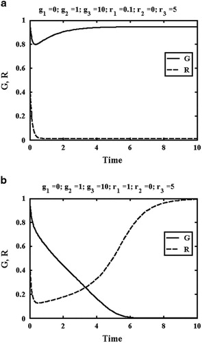
Where A=r₁/g₃, B=R₀−r₁/g₃, C=1−r₁r₃/g₂g₃ and D=(g₃r₃R₀−r₁r₃)/(g₃²−g₂g₃). The steady-state levels must then be R=r₁/g₃ (here, 0.01) and G=1−r₁r₃/g₂g₃ (0.95). These values are not functions of the initial conditions. Many parameter choices give similar results, with the government re-establishing control. However, some give a different outcome. For example, Figure 1b shows results for , G₀=1 and R₀=0.5. The only change from Figure 1a is a large increase in the rebel recruitment term r₁. However, the effect is dramatic: the government is annihilated, and the rebel force rises to unity. Clearly, the possibility of a revolution is inherent in the equations. However, systematic investigation is needed to establish when it can occur.

3. Phase plane analysis

Non-linear coupled differential equations are often analysed on a plane whose axes are the two variables. Here, dG/dt>0 when G=0, and dG/dt<0 when G=1; similarly, dR/dt>0 when R=0, and dR/dt<0 when R=1. Consequently, only the region bounded by G=0, G=1, R=0 and R=1 need be considered, as solutions starting in this region must remain inside it. Null isoclines are obtained when dG/dt=0 or dR/dt=0, or when

Equation (7) are smooth curves and points of equilibrium with co-ordinates (G_e, R_e) are obtained where they intersect.For R_e, this leads to the quartic equation:

Here a₁=g₂r₁, b₁=g₁g₃+g₂(r₂−r₁), c₁=−g₂r₂, a₂=−r₁, b₂=g₃+r₁−r₂, c₂=r₂, a₃=g₃r₁r₃, b₃=g₃(r₂−r₁)r₃ and c₃=−g₃r₂r₃. Generally, there will be four roots. However, a special case is obtained when g₁=0 and r₂=0. In this case, the quartic reduces to the cubic:

One solution is R_e=1 and G_e=0, which corresponds to a rebel win accompanied by government annihilation as shown in Figure 1b. The others are the roots of the bracketed quadratic:

When r₁ is small, the smaller root approximates to R_e≈r₁/g₃ and G_e≈1−r₁r₃/g₂g₃, the steady state values of Equation (6). Consequently, a second state has the Government firmly in control, but with an undercurrent of rebel activity as in Figure 1a. The character of the third state will become clear later. Repeated roots are obtained when g₂²(g₃+r₁)²−4g₂g₃r₁r₃=0, which requires:

Repeated roots can never be obtained if r₃<g₂, because the required value of r₁ is complex. However, if r₃>g₂, we would expect a change in equilibria when r₁ reaches a critical value.

Standard techniques are used to analyse the nature of any equilibrium point (G_e, R_e). Lyapunov’s indirect method involves linearising the equations in the vicinity. Introducing new variables ΔG=G−G_e and ΔR=R−R_e, where ΔG and ΔR are small, the resulting equations can be written as Here is the column vector (ΔG, ΔR) and is the Jacobian matrix:

Now, will have eigenvalues λ₁ and λ₂ and eigenvectors and and a solution for initial conditions at t=0 can always be written in terms of these eigenvalues and eigenvectors. An arbitrary perturbation will then decay to zero (so the equilibrium is stable) if both λ₁ and λ₂ have negative real parts. Other possibilities can be classified as follows. The eigenvalues are λ_1,2={Tr±√[Tr²−4Det]}/2, where Tr=J₁₁+J₂₂ is the trace of and Det=J₁₁J₂₂−J₁₂J₂₁ is its determinant. The eigenvalues will therefore be complex if the discriminant Tr²−4Det is negative. In this case, the trajectories will be spirals that tend towards or away from the equilibrium. If the discriminant is positive, simpler nodes are obtained. If Det<0, the discriminant must be real, and the eigenvalues of opposite sign, so the equilibrium is a saddle. If Det>0, the eigenvalues must have the same sign. If Tr>0, both must be positive, and the equilibrium is an unstable focus. If Tr<0, both must be negative and the equilibrium is a stable focus.

Alternative behaviour can arise in the form of limit cycles, whose existence or absence can be established using the Poincaré–Bendixson and Bendixson–Dulac theorems. In the notation here, the latter requires identification of a differentiable function h such that ∂(hf_G)/∂G+∂(hf_R)/∂R has the same sign (≠0) in a simply connected region. A suitable function here is h=G⁻¹R⁻¹, which leads to:

Since the coefficients are all positive, the right-hand side is always negative in the first quadrant, so there can be no limit cycles in this region, whatever the coefficient values.

4. Stable and unstable regimes

We now present numerical examples. To begin with, we assume to represent a government with no popular support, but plentiful resources and weapons. Similarly, we assume to represent rebels with modest support, no resources and a weaker arsenal. The thick lines in Figure 2a are the null isoclines, while the discrete points indicate equilibria. The isoclines are straight for the government and hyperbolic for the rebels. Trajectories must cross the government isocline vertically, and the rebel isocline horizontally. There are three equilibria in the region, Point A at (0, 1), and B and C at the two solutions to Equation (5). Lyapunov analysis shows that A and C are stable foci, while B is a saddle point. The thin lines in Figure 2b show representative trajectories, starting from the perimeter. Trajectories clearly skirt the unstable equilibrium point B, and end only at the stable equilibria A and C. Those ending at C with the government dominating are shown as full lines, while those ending at A with the rebels dominant are dashed. In this example, the government remains in control except when the rebels initially outnumber them (an unrealistic situation), so these parameters represent a stable, oppressive government. Points A and C correspond to states of competitive exclusion in a biological model. However, in this case, the equations would be in Kolmogorov form, with r₁ zero and r₂ non-zero. Both isoclines would then be straight, and the state with government dominant would also have the rebels extinct, eliminating any possibility for future revolution. Thus, the coefficient r₁ allows perpetual opposition.

Figure 2 (a) Example null isoclines and equilibrium states and (b) phase portraits for a government in power, with minor unrest.

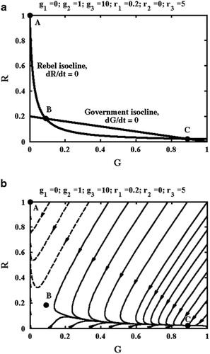
Other parameter combinations can result in stalemate. However, because stalemates have been considered extensively elsewhere (MacKay, 2014), we focus here on exclusion scenarios, and particularly on the effect of r₁ in altering the outcome. For example, Figure 3a shows results for and Here all parameters are unchanged, except r₁, which has increased. As a result, the rebel isocline has risen, points B and C have moved closer together, and the phase portrait has fewer full-line trajectories. The net effect is to imply weaker government control. A similar effect is obtained if g₂ and g₃ are reduced (which corresponds to decay of the regime), but this time it is the government isocline that alters, by reducing its slope.

Figure 3 Example null isoclines (thick, full lines), equilibrium states (points) and phase portraits (thin, full and dashed lines) for a government initially in power, with (a) major unrest and (b) rebels gaining power.

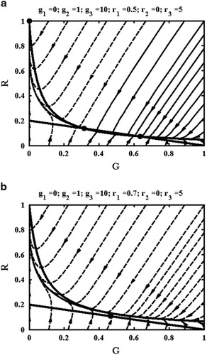
Equation (11) implies that points B and C will coincide at a critical value of r₁, and then become complex conjugates. For the previous parameters, the smaller solution is r₁=0.557. Figure 3b shows the results when and so r₁ is well above this value. There are now no intersections of the isoclines. Although an equilibrium point is shown, it is only the real part of a complex conjugate pair. As a result, the phase portrait only contains dashed-line trajectories ending at the rebel win condition. Consequently, the government will always lose control, the condition for revolution.

At this point we note that assignment of government characteristics to G and rebel characteristics to R is arbitrary. G and R are just the current government and rebels, and the situation might one day be reversed, with R in power and G seeking it. In that case, more relevant titles for the two sides might be green and red. However, transfer of power from R to G can take place by exactly the same mechanism.

5. Cyclic regime change

We now consider the modifications needed to allow cyclic regime change. Since our constant–coefficient model forbids cycles, the answer must lie in changes in behaviour. Behavioural variations are well known in biology, and competition equations have been made more realistic, by allowing switching of a predator between prey, or prey between habitats. Often, this behaviour is modelled using sigmoidal functions, which can switch a coefficient on or off depending on the size of the population. Switching might be expected in human behaviour, and sigmoidal functions have already been used in a conflict model (Feichtinger and Forst, 1996). Here, the variations depend on choices made after a revolution. More precisely, since the goal of most rebels will have simply been to remove the government, they will depend on the decisions of the rebel leaders.

Almost certainly, successful rebels will seize the resources and weapons of the previous regime. Depending on the degree of temporary disorder, they may re-employ many of its mercenaries. When order is restored, the leaders may be tempted to enjoy the lifestyle of the previous regime, and indeed this may have been their aim all along. If this is the case, the grievance of the majority will be rapidly displaced by the greed of an opportunistic minority. However, this enhanced lifestyle is necessarily exploitative. If, to maintain it, the rebels deploy their new assets against the larger population, they will sooner or later lose its support. Similarly, the deposed government will immediately lose its resources. However, either it or a similarly disenchanted group may after a while acquire popular support and the weapons needed to mount another revolution. If these changes occur, each competitor will after a time assume the characteristics of the other. However, the switching characteristics cannot simply be a function of the current state. For example, while it is in power, a government is likely to retain its assets until it falls. However, when attempting to regain power, it will not recover them until it succeeds. Consequently, switching cannot involve mere reversal of history; hysteresis must be involved.

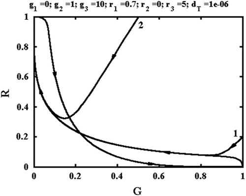
A suitable algorithm may be constructed as follows. Whenever a new stable state is reached (defined by G or R approaching unity to within a threshold d_T), generate new coefficient vectors and from old vectors and following , . Figure 4 shows the phase portrait starting at Point 1=(1, 0.2), assuming initial coefficient vectors , and d_T=10⁻⁶. Here G is in power, but the coefficients are such that a revolution is inevitable and the trajectory sweeps to (0, 1). Once R is in power, however, it rapidly becomes oppressive itself and after a while generates the conditions for a new revolution ending at (1, 0). Each time a revolution occurs, those coming to power make the same mistakes and the scenario repeats. The effect is to generate a self-intersecting cycle between (1, 0) and (0, 1), and alternative initial conditions such as Point 2 yield trajectories that cross part of the cycle before joining it.

Figure 4 Phase portrait for a cycle of revolutions following from two different initial conditions.

Changes to the parameters mainly affect the cycle time, rather than the shape of the loop. The only chance of avoiding this cycle is if successful revolutionaries are more egalitarian. Instead of immediately adopting a lifestyle so luxurious that it must be defended by force, they should share the proceeds of victory. In doing so, they will reduce the grievance that leads to revolution, and the temptation for future governments to become oppressive. One possibility is a democracy, which has mechanisms to avoid concentrated wealth and power. Unfortunately, because the necessary choices are sub-optimal for those in power, democracies are rare.

6. Discussion

In this section, we examine in more detail some key aspects of the model. Particularly, we consider the assumptions that (i) the government and rebels are both predators, (ii) the coefficients in the differential equations are constant and (iii) switching between rebel- and government-type behaviour is instantaneous. We also ask how the numerical values of the coefficients might be established, and suggest possible directions for further research.

(i) Predatory behaviour

The predatory nature of many regimes is well established, and there is evidence that their number is increasing (Diamond, 2008). There is also strong evidence that many rebels are predatory, that their aim is often loot seeking (Gates, 2002), and that they may not even need a successful rebellion to set up a parasitic internal economy (Suarez, 2000). In fact, Collier (2000) considers rebellion to be a branch of criminal activity, where the government and rebels both act as predators on natural resource rents. Such behaviour is prevalent in regions with gemstone or drugs wealth (Olsson, 2007), so that these are often torn by civil war. Oil resources are intrinsically less lootable and require capital-intensive infrastructure. However, if this is available, revenue sharing with a client elite can extend the longevity of kleptocratic regimes (Crespo Cuaresma et al, 2011). Finally, where regime change has recently occurred, it has hardly ever led to democracy (Albrecht, 2004), and competitive predatory activities are rampant in transition economies (Mehlum et al, 2003).

(ii) The nature of the differential equation coefficients

We have assumed that all the coefficients are constant before a rebellion. Of course, this is an extreme simplification. For example, insurgents often adopt terrorist tactics aimed at forcing a disproportionate response and consequently enhancing popular support (Merari, 1993; Kydd and Walter, 2006). Such effects are partly embedded in the existing model, so that strong public sympathy may be indicated by a large value of the coefficient r₁. However, realism may be improved by making r₁ depend on the level of government killings, for example by assuming that r₁=r_1a+r_1b(g₃GR). Conversely, the government may respond to rebel attacks by increasing repression (Gartner and Regan, 1996). This effect might be incorporated by making g₃ depend on the level of rebel killings, for example by taking g₃=g_3a+g_3b(r₃RG). We have carried out simulations with r₁ and g₃ modified as described, and find that the main effect of r_1b is to reduce the threshold value of r_1a needed for a rebellion, while the effect of g_3b is to reduce the value of g_3a needed to prevent one.

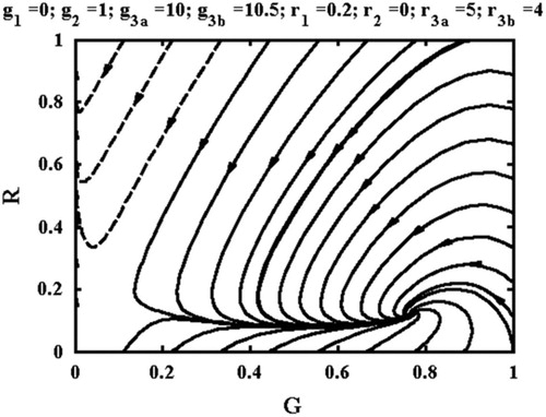
Other possibilities include making each side respond to the perceived situation. For example, it has been suggested that attitudes to risk evolve in winner-takes-all games, so that the more a player has to lose, the more prone they are to high-risk strategies. Government violence increasing with perceived weakness might be incorporated by making g₃ increase as G reduces, as g₃=g_3a−g_3aG. Note that if g_3b>g_3a, this implies that g₃ may become negative for sufficiently large G. This effect might correspond to a strong government releasing political prisoners. In a similar way, rebel daring increasing as G reduces might be modelled by assuming r₃=r_3a−r_3aG. These assumptions do make a significant difference. For example, Figure 5 shows a phase-plane portrait for g₂=1, g_3a=10, g_3b=10.5, r₁=0.2, r_3a=5 and r_3b=4. These parameters match Figure 2, apart from the introduction of g_3b and r_3b. Their effect is to convert the stable node at the government win condition into a stable spiral, introducing the oscillations in coercion and dissidence noted by Tsebelis and Sprague (1989). However, as before, a revolution may still occur if r₁ is large enough. Other changes may yield entirely different results, because they add extra non-linear terms to the equations. Existing equilibria may change from stable to unstable, and additional equilibria or limit cycles may be introduced. Consequently, any such alterations must be studied carefully.

Figure 5 Phase portrait for government in power, but with government and rebels both playing a reactive strategy depending on G.

(iii) The values of the differential equation coefficients

We have assumed arbitrary recruitment and attrition coefficients. An important question is whether their values could be established for realistic situations. In combat modelling, considerable attention was paid to attrition from the start (see eg Helmbold’s translation of Osipov’s 1915 studies). Recent conventional battles have also been examined (Bracken, 1995), as have civil wars (Weiss, 1966). A key difficulty is lack of data. These are typically only available as final casualties, and even then often only for the winning side, making it difficult to model extended conflicts (Lucas and Dinges, 2004). Recruitment has received less attention, although force requirements for military operations have been considered (Taylor, 1983), most recently for counter-insurgency (Goode, 2009). Military operations at least have the advantage that data are required for logistics or public accountability. However, in a rebellion, there is likely to be a reluctance to keep records on both sides. Government recruitment might be estimated from leaked payroll data, and security force casualties from news records. Rebel recruitment is by its nature clandestine, and the numbers of political prisoners and executions are generally withheld, although data may be available from monitors such as Human Rights Watch and Amnesty International. Some success has been achieved in matching dynamic theories to records of protests (Francisco, 1995); however, the gathering of suitable data is likely to be a promising field for future research.

(iv) The nature of the switching algorithm

We have assumed abrupt switching between rebel- and government-type behaviour following a successful revolution. Synchronous changes are clearly not likely. Seizure of weapons and regime assets will inevitably be rapid, so that switching of r₂ and g₂, and r₃ and g₃ might be expected immediately after a revolution. However, the larger population will take some time to understand the exact nature of any regime change. Even when it has, and the conclusion is unfavourable, appetite for a further revolution will certainly be low when one has just occurred. Thus, we would expect switching of the coefficients r₁ and g₁ to take place later. However, this refinement is likely to alter the shape of the limit cycle only near the points (1, 0) and (0, 1). Exact switching is also clearly implausible. Many of the actors will change; particularly, the new rebels will not correspond exactly to the old security forces. Some of the latter may be killed or imprisoned in acts of reprisal, while others may be hired into the new security forces. The new rebels are therefore likely to be a different set of opportunistic predators. As a result, closed cycles will not be obtained and the limit cycle in Figure 4 will become blurred. However, despite these details, it does seem reasonable that response switching is responsible for at least some of the repetitive dynamics of history.

(v) Possible extensions

There are clearly many possible extensions to the model that could be incorporated, particularly to describe outside interference, foreign-imposed regime change and proxy war. Some might take the form of further functional responses. For example, International condemnation of the government and subsequent denial of arms deliveries might appear as a reduction in g₃ depending on government behaviour. Similarly, sympathy for the rebels materialising in external financial assistance or supply of weapons might be accounted for by increases in r₂ and r₃. Other changes might involve the addition of extra parties. The host or neutral population could be considered, together with foreign forces on either side. However, as population biologists and, in this context, Feichtinger and Forst (1996) have noted, the addition of even one extra species can again have a dramatic effect on stability and survival, and greatly complicate graphical presentation. Such extensions should therefore be attempted only when simpler models are thoroughly understood.

7. Conclusions

A differential model for rebellion against an oppressive government has been proposed. The coefficient values represent the three main aspects of the struggle: popular support, resources and weapons. Depending on their values, the model allows scenarios that demonstrate stable oppressive government and its overthrow. With constant coefficients, limit cycles are not obtained. However, cycles emerge if rebels and failed regimes are allowed to alter their behaviour by exchanging coefficients after a successful revolution. These changes can be accounted for partly by seizure of regime assets and partly by changes in rebel motivation from grievance to greed. Effectively, therefore, they describe the hijacking of a revolution.

Acknowledgements

We would like to thank the two anonymous referees for their helpful and stimulating comments.