Containment of socially optimal policies in multiple-facility Markovian queueing systems

Abstract

We consider a Markovian queueing system with N heterogeneous service facilities, each of which has multiple servers available, linear holding costs, a fixed value of service and a first-come-first-serve queue discipline. Customers arriving in the system can be either rejected or sent to one of the N facilities. Two different types of control policies are considered, which we refer to as ‘selfishly optimal’ and ‘socially optimal’. We prove the equivalence of two different Markov Decision Process formulations, and then show that classical M/M/1 queue results from the early literature on behavioural queueing theory can be generalized to multiple dimensions in an elegant way. In particular, the state space of the continuous-time Markov process induced by a socially optimal policy is contained within that of the selfishly optimal policy. We also show that this result holds when customers are divided into an arbitrary number of heterogeneous classes, provided that the service rates remain non-discriminatory.

Keywords:

• queues with balking
• Markov Decision Processes
• equilibrium strategies
• optimal strategies
• dynamic programming

after two revisions

The online version of this article is available Open Access

1. Introduction

One of the most persistent themes in the literature on behavioural queueing theory is the sub-optimality of greedy or ‘selfish’ customer behaviour in the context of overall social welfare. In order to induce the most favourable scenario for society as a whole, customers are typically required to deviate in some way from the actions that they would choose if they were motivated only by their own interests. This principle has been observed in many of the classical queueing system models, including M/M/1, GI/M/1, GI/M/s and others (see, eg, Naor, 1969; Yechiali, 1971; Knudsen, 1972; Yechiali, 1972; Littlechild, 1974; Edelson and Hildebrand, 1975; Lippman and Stidham, 1977; Stidham, 1978). More recently, this theme has been explored in applications including queues with setup and closedown times (Sun et al, 2010), queues with server breakdowns and delayed repairs (Wang and Zhang, 2011), vacation queues with partial information (Guo and Li, 2013), queues with compartmented waiting space (Economou and Kanta, 2008) and routing in public services (Knight et al, 2012; Knight and Harper, 2013). More generally, the implications of selfish and social decision making have been studied in various applications of economics and computer science; Roughgarden’s (2005) monograph provides an overview of this work and poses some open problems.

The first author to compare ‘self-optimization’ with ‘overall optimization’ in a queueing setting was Naor (1969), whose classical model consists of an M/M/1 system with linear waiting costs and a fixed service value. The general queueing system that we consider in this paper may be regarded as an extension of Naor’s model to a higher-dimensional space. We consider a system with N⩾2 heterogeneous service facilities in parallel, each of which has its own queue and operates with a cost and reward structure similar to that of Naor’s single-server model (see Figure 1). In addition, we generalize the system by assuming that each facility i may serve up to c_i customers simultaneously, so that we are essentially considering a network of non-identical M/M/c_i queues.

Figure 1 A diagrammatic representation of the queueing system.

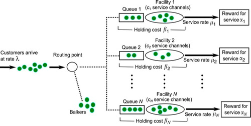
The inspiration for our work is derived primarily from public service settings in which customers may receive service at any one of a number of different locations. For example, in a healthcare setting, patients requiring a particular operation procedure might choose between various different healthcare providers (or a choice might be made on their behalf by a central authority). In this context, the ith provider is able to treat up to c_i patients at once, and any further arrivals are required to join a waiting list, or seek treatment elsewhere. A further application of this work involves the queueing process at immigration control at ports and/or airports. These queues are often centrally controlled by an officer aiming to ensure that congestion is reduced. Finally, computer data traffic provides yet another application of this work. When transferring packets of data over a network, there arise instances at which choices of available servers can have a major impact on the efficacy of the entire network.

The queueing system that we consider in this work evolves stochastically according to transitions which we assume are governed by Markovian distributions. We address the problem of finding an optimal routing and admission control policy and model this as a Markov Decision Process (MDP) (see, eg, Puterman, 1994) for a complete description and rigorous theoretical treatment of MDPs). Stidham and Weber (1993) provide an overview of MDP models for the control of queueing networks. It is well-known that optimal policies for the allocation of customers to parallel heterogeneous queues are not easy to characterize; for this reason, heuristic approaches have been developed which have achieved promising results in applications (see Argon et al, 2009; Glazebrook et al, 2009). In attempting to identify or approximate an optimal policy, one aims to find a dynamic decision-making scheme which optimizes the overall performance of the system with respect to a given criterion; we refer to such a scheme as a socially optimal solution to the optimization problem associated with the MDP. In this paper our objective is to draw inferences about the nature of a socially optimal solution from the structure of the corresponding selfishly optimal solution. A selfishly optimal solution may be regarded as a simple heuristic rule which optimizes a customer’s immediate outcome without giving due consideration to long-term consequences. The remaining sections in this paper are organized as follows:

• In Section 2 we provide an MDP formulation of our queueing system and define all of the input parameters. We also offer an alternative formulation and show that it is equivalent.

• In Section 3 we define ‘selfishly optimal’ and ‘socially optimal’ policies in more detail. We then show that our model satisfies certain conditions which imply the existence of a stationary socially optimal policy, and prove an important relationship between the structures of the selfishly and socially optimal policies.

• In Section 4 we draw comparisons between the results of Section 3 and known results for systems of unobservable queues.

• In Section 5 we show that the results of Section 3 hold when customers are divided into an arbitrary number of heterogeneous classes. These classes are heterogeneous with respect to demand rates, holding costs and service values, but not service rates.

• Finally, in Section 6, we discuss the results of this paper and possible avenues for future research.

2. Model formulation

We consider a queueing system with N service facilities. Customers arrive from a single demand node according to a stationary Poisson process with demand rate λ>0. Let facility i (for i=1, 2, …, N) have c_i identical service channels, a linear holding cost β_i>0 per customer per unit time, and a fixed value of service (or fixed reward) α_i>0. Service times at any server of facility i are assumed to be exponentially distributed with mean μ_i⁻¹. We assume α_i⩾β_i/μ_i for each facility i in order to avoid degenerate cases where the reward for service fails to compensate for the expected costs accrued during a service time. When a customer arrives, they can proceed to one of the N facilities or, alternatively, exit from the system without receiving service (referred to as balking). Thus, there are N+1 possible decisions that can be made upon a customer’s arrival. The decision chosen is assumed to be irrevocable; we do not allow reneging or jockeying between queues. The queue discipline at each facility is first-come-first-served (FCFS). A diagrammatic representation of the system is given in Figure 1.

We define to be the state space of our system, where x_i (the ith component of the vector x) is the number of customers present (including those in service and those waiting in the queue) at facility i. It is assumed that the system state is always known and can be used to inform decision making.

No binding assumption is made in this paper as to whether decisions are made by individual customers themselves, or whether actions are chosen on their behalf by a central controller. It is natural to suppose that selfish decision making occurs in the former case, whereas socially optimal behaviour requires some form of central control, and the discussion in this paper will tend to be consistent with this viewpoint; however, the results in this paper remain valid under alternative perspectives (eg, socially optimal behaviour might arise from selfless co-operation between customers).

We do not assume any upper bound on the value of λ in terms of the other parameters. However, the types of policies that we consider in this work always induce system stability. For convenience, we will use the notation xⁱ⁺ to denote the state which is identical to x except that one extra customer is present at facility i; similarly, when x_i⩾1, we use xⁱ⁻ to denote the state with one fewer customer present at facility i. That is:

where e_i is the ith vector in the standard orthonormal basis of

Let us discretize the system by defining:

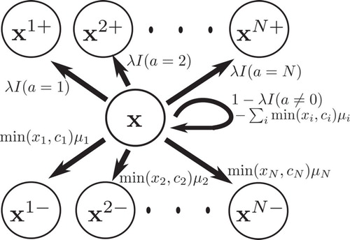
and considering an MDP which evolves in discrete time steps of size Δ. Using the well-known technique of uniformization, usually attributed to Lippman (1975) (see also Serfozo, 1979), we can analyse the system within a discrete-time framework, in which arrivals and service completions occur only at the ‘jump times’ of the discretized process. At any time step, the probability that a customer arrives is λΔ, and the probability that a service completes at facility i is either c_iμ_iΔ or x_iμ_iΔ, depending on whether or not all of the channels at facility i are in use. At each time step, an action a∈{0, 1, 2, …, N} is chosen which represents the destination of any customer who arrives at that particular step; if a=0 then the customer balks from the system, and if a=i (for i∈{1, 2, …, N}) then the customer joins facility i. This leads to the following definition for the transition probabilities p_xy(a) for transferring from state x to y in a single discrete time step, given that action a is chosen:

Here we have used I to denote the indicator function. Since the units of time can always be re-scaled, we may assume Δ=1 without loss of generality, and we therefore suppress Δ in the remainder of this work. Figure 2 illustrates these transition probabilities diagrammatically.

Figure 2 Transition probabilities (marked next to arrows) from an arbitrary state x∈S.

If the system is in some state x∈S at a particular time step, the sum of the holding costs incurred is Σ_i=1^Nβ_ix_i; meanwhile, services are completing at an overall rate Σ_i=1^Nmin(x_i, c_i)μ_i and the value of service at facility i is α_i. This leads to the following definition for the single-step expected net reward r(x) associated with being in state x at a particular time step:

The system may be controlled by means of a policy which determines, for each the action a_n to be chosen after n time steps. In this paper we focus on stationary non-randomized policies, under which the action a_n is chosen deterministically according to the accompanying system state x_n, and is not dependent on other factors (such as the history of past states and actions, or the time index n). In Section 3 it will be shown that it is always possible to find a policy of the aforementioned type which achieves optimality in our system. Let x_n and a_n be, respectively, the state of the system and accompanying action chosen after n time steps, and let us use θ to denote the stationary policy being followed. The long-run average net reward g_θ(x, r) per time step, given an initial state x₀=x and reward function r, is given by:

where the dependence of x_n on the previous state x_n−1 and action a_n−1 is implicit. Before proceeding, we will show that an alternative definition of the reward function r yields the same long-run average reward (assuming that the same policy is followed). If a customer joins facility i under system state x, then their individual expected net reward, taking into account the expected waiting time, holding cost β_i and value of service α_i, is given by α_i−β_i/μ_i if they begin service immediately, and α_i−β_i(x_i+1)/(c_iμ_i) otherwise. Given that the probability of a customer arriving at any time step is λ, this suggests the possibility of a new reward function which (unlike the function r defined in (1)) depends on the chosen action a in addition to the state x:

The two reward functions in (1) and (3) look very different at first sight, but both formulations are entirely logical. The original definition in (1) is based on the real-time holding costs and rewards accrued during the system’s evolution, while the alternative formulation in (3) is based on an unbiased estimate of each individual customer’s contribution to the aggregate net reward, made at the time of their entry to the system. We will henceforth refer to the function r in (1) as the real-time reward function, and the function in (3) as the anticipatory reward function. Our first result proves algebraically that these two reward formulations are equivalent.

Lemma 1

• For any stationary policy θ we have:

  where r andare defined as in (1) and (3) respectively. That is, the long-run average net reward under θ is the same under either reward formulation.

Proof

• We assume the existence of a stationary distribution {π_θ(x)}_x∈S, where π_θ(x) is the steady-state probability of being in state x∈S under the stationary policy θ and ∑_x∈Sπ_θ(x)=1. If no such distribution exists, then the system is unstable under θ and both quantities in (4) are infinite. Under steady-state conditions, we can write:

  noting, as before, that (unlike r) has a dependence on the action θ(x) associated with x. For each x∈S, the steady-state probability π_θ(x) is the same under either reward formulation since we are considering a fixed stationary policy. Our objective is to show:

  We begin by partitioning the state space S into disjoint subsets. For each facility i∈{1, 2, …, N}, let S_i denote the (possibly empty) set of states at which the action chosen under the policy θ is to join i. Then S_i=S_i−∪S_i+, where:

  We also let S₀ denote the set of states at which the action chosen under θ is to balk. Now let g_θ (x, r) and be divided into ‘positive’ and ‘negative’ constituents in the following way:

  By referring to (1) and (3), it can be checked that g_θ(x,r)=g_θ⁺(x,r)+g_θ⁻(x,r) and It will be sufficient to show that and . Let S_i,k⊆S_i (for k=0, 1, 2, …) be the set of states at which the action chosen under θ is to join facility i, given that there are k customers present there. That is:

  Using the detailed balance equations for ergodic Markov chains under steady-state conditions (see, eg, Cinlar, 1975) we may assert that for every facility i and k⩾0, the total flow from all states x∈S with x_i=k up to states with x_i=k+1 must equal the total flow from states with x_i=k+1 down to x_i=k. Hence:

  Summing over all , we obtain:

  which holds for i∈{1, 2, …, N}. The physical interpretation of (6) is that, under steady-state conditions, the rate at which customers join facility i is equal to the rate at which service completions occur at i. Multiplying both sides of (6) by α_i and summing over i∈{1, 2, …, N}, we have:

  which states that as required. It remains for us to show that We proceed as follows: in (5) (which holds for all and i∈{1, 2, .., N}), put k=c_i to obtain:

  Suppose we multiply both sides of (7) by c_i+1. Since the sum on the left-hand side is over and the sum on the right-hand side is over states with x_i=c_i+1, this is equivalent to multiplying each summand on the left-hand side by x_i+1 and each summand on the right-hand side by x_i. In addition, multiplying both sides by β_i/(c_iμ_i) yields:

  We can write similar expressions with k=c_i+1, c_i+2 and so on. Recall that by definition. Hence, by summing over all k⩾c_i in (8) we obtain:

  Note also that multiplying both sides of (5) by β_i/μ_i and summing over all k<c_i (and recalling that ) gives:

  Hence, from (9) and (10) we have:

  Summing over i∈{1, 2, …, N} gives as required. We have already shown that so this completes the proof that . □

It follows from Lemma 1 that any policy which is optimal among stationary policies under one reward formulation (either r or ) is likewise optimal under the other formulation, with the same long-run average reward. The interchangeability of these two reward formulations will assist us in proving later results.

3. Containment of socially optimal policies

Let us define what we will refer to as ‘selfishly optimal’ and ‘socially optimal’ policies. The terminology used in this paper is slightly incongruous to that which is typically found in the literature on MDPs, and the main reason for this is that we wish to draw analogies with the work of Naor (1969). The policies which we describe as ‘socially optimal’ are those which satisfy the well-known Bellman optimality equations of dynamic programming (introduced by Bellman, 1957), and would be referred to by many authors simply as ‘optimal’ policies; on the other hand, the ‘selfishly optimal’ policies that we will describe could alternatively be referred to as ‘greedy’ or ‘myopic’ policies.

We begin with selfishly optimal policies. Suppose that each customer arriving in the system is allowed to make his or her own decision (as opposed to being directed by a central decision-maker). It is assumed throughout this work that the queueing system is fully observable and therefore the customer is able to observe the exact state of the system, including the length of each queue and the occupancy of each facility (the case of unobservable queues is a separate problem; see, eg, Bell and Stidham, 1983; Haviv and Roughgarden, 2007; Shone et al, 2013). Under this scenario, a customer may calculate their expected net reward (taking into account the expected cost of waiting and the value of service) at each facility based on the number of customers present there using a formula similar to (3); if they act selfishly, they will simply choose the option which maximizes this expected net reward. If the congestion level of the system is such that all of these expected net rewards are negative, we assume that the (selfish) customer’s decision is to balk. This definition of selfish behaviour generalizes Naor’s simple decision rule for deciding whether to join or balk in an M/M/1 system. We note that since the FCFS queue discipline is assumed at each facility, a selfish customer’s behaviour depends only on the existing state, and is not influenced by the knowledge that other customers act selfishly.

Taking advantage of the ‘anticipatory’ reward formulation in (3), we can define a selfishly optimal policy by:

In the case of ties, we assume that the customer joins the facility with the smallest index i; however, balking is never chosen over joining facility i when This is in keeping with Naor’s convention.

A socially optimal policy, denoted θ*, is any policy which maximizes the long-run average net reward defined in (2). The optimality equations for our system, derived from the classical Bellman optimality equations for average reward problems (see, eg, Puterman, 1994) and assuming the real-time reward formulation in (1), may be expressed as:

where h(x) is a relative value function and g* is the optimal long-run average net reward. (We adopt the notational convention that x⁰⁺=x to deal with the case where balking is optimal in (11).) Under the anticipatory reward formulation in (3) these optimality equations are similar except that r(x) is replaced by , which must obviously be included within the maximization operator. Indeed, by adopting as our reward formulation we may observe the fundamental difference between the selfishly and socially optimal policies: the selfish policy simply maximizes the immediate reward , without taking into account the extra term h(x^a+); this is why it may be called a myopic policy. The physical interpretation is that under the selfish policy, customers consider only the outcome to themselves, without taking into account the implications for future customers, who may suffer undesirable consequences as a result of their behaviour.

In this work we assume an infinite time horizon, but we use the method of successive approximations (see Ross, 1983) to treat the infinite horizon problem as the limiting case of a finite horizon problem. We therefore state the finite horizon optimality equations corresponding to the infinite horizon equations in (11):

where v*_n(x) is the maximal expected total reward from a problem with n time steps, given an initial state x∈S (we define v*₀(x)=0 for all x∈S).

Remark

• It has already been shown (Lemma 1) that, in an infinite-horizon problem, a stationary policy earns the same long-run average reward under either of the reward formulations r and . However, this equivalence is lost when we consider finite-horizon problems. Indeed, given a finite horizon n, a policy which is optimal under reward function r may perform extremely poorly under This is especially likely to be the case if n is small.

Given that selfish customers refuse to choose facility i if it follows that for i=1, 2, …, N there exists an upper threshold b_i which represents the greatest possible number of customers at i under steady-state conditions. The value b_i can be derived from (3) as:

where denotes the integer part. Two important ways in which the selfishly optimal policy differs from a socially optimal policy are as follows:

1. The decisions made under are entirely independent of the demand rate λ.

2. The threshold b_i (representing the steady-state maximum occupancy at i) is independent of the parameters for the other facilities j≠i.

Because of the thresholds b_i, a selfishly optimal policy induces an ergodic Markov chain defined on a finite set of states Formally, we have:

We will refer to as the selfishly optimal state space. Note that, due to the convention that the facility with the smallest index i is chosen in the case of a tie between the expected net rewards at two or more facilities, the selfishly optimal policy is unique in any given problem. Changing the ordering of the facilities (and thereby the tie-breaking rules) affects the policy but does not alter the boundaries of

Let denote the set of positive recurrent states belonging to the Markov chain induced by a socially optimal policy θ* satisfying the optimality equations in (11). The main result to be proved in this section is that is not only finite, but must also be contained in .

Example 1

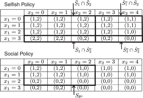
• Consider a system with demand rate λ=12 and only two facilities. The first facility has two channels available (c₁=2) and a service rate μ₁=5, holding cost β₁=3 and fixed reward α₁=1. The parameters for the second facility are c₂=2, μ₂=1, β₂=3 and α₂=3, so it offers a higher reward but a slower service rate. We can uniformize the system by taking Δ=1/24, so that (λ+∑_ic_iμ_i)Δ=1. The selfishly optimal state spacefor this system consists of 12 states.Figure 3shows the decisions taken at these states under the selfishly optimal policyand also the corresponding decisions taken under a socially optimal policy θ*.

  Figure 3 Selfishly and socially optimal policies for Example 1.

  Note: For each state , the corresponding decisions under the respective policies are shown.

  

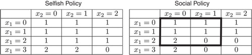
  By comparing the tables in Figure 3 we may observe the differences between the policiesandθ*. At the states (2, 0), (2, 1), (2, 2) and (3, 1), the socially optimal policyθ* deviates from the selfish policy (incidentally, the sub-optimality of the selfish policy is about 22%). More striking, however, is the fact that under the socially optimal policy, some of the states in are actually unattainable under steady-state conditions. Indeed, the recurrent state space consists of only six states (enclosed by the bold rectangle in the figure). Thus, for this system, and in this section we aim to prove that this result holds in general.

It is known that for a general MDP defined on an infinite set of states, an average reward optimal policy need not exist, and that even if such a policy exists, it may be non-stationary. In 1983, Ross provides counter-examples to demonstrate both of these facts. Thus, it is desirable to establish the existence of an optimal stationary policy before aiming to examine its properties. Our approach in this section is based on the results of Sennott (1989), who has established sufficient conditions for the existence of an average reward optimal stationary policy for an MDP defined on an infinite state space (this problem has also been addressed by other authors; see, eg, Zijm, 1985; Cavazos-Cadena, 1989). We will proceed to show that Sennott’s conditions are satisfied for our system, and then deduce that for any socially optimal policy θ*, must be contained in Sennott’s approach is based on the theory of discounted reward problems, in which a reward earned n steps into the future is discounted by a factor γⁿ, where 0<γ<1. A policy θ is said to be γ-discount optimal if it maximizes the total expected discounted reward (abbreviated henceforth as TEDR) over an infinite time horizon, defined (for reward function ) as:

Let θ^*_γ denote an optimal policy under discount rate γ, and let be the corresponding TEDR, so that It is known that satisfies the discount optimality equations (see Puterman, 1994):

We proceed to show that in our system, the discount optimal value function v*_γ satisfies conditions which are sufficient for the existence of an average reward optimal stationary policy. In the proofs of the upcoming results, we adopt the anticipatory reward function defined in (3).

Lemma 2

• For every statex∈S and discount rate 0<γ<1:

Proof

• Let θ₀ be the trivial policy of balking under every state. Each reward is zero and hence . Since by definition, the result follows.  □

The next result establishes an important monotonicity property of the function which, incidentally, does not hold for its counterpart under the real-time reward formulation (1).

Lemma 3

• For every statex∈S, discount rate 0<γ<1 and facility i∈{1, 2, …, N}, we have:

Proof

• We rely on the finite horizon optimality equations (for discounted problems) and prove the result using induction on the number of stages. The finite horizon optimality equations are:

  It is sufficient to show that for each state x∈S, discount rate 0<γ<1, facility i∈{1, 2, …, N} and integer n⩾0:

  We define for all x∈S. In order to show that (16) holds when n=1, we need to show, for i=1, 2, …, N:

  Indeed, let . It follows from the definition of in (3) that for any fixed action a and facility i. Hence:

  Now let us assume that (16) also holds for n=k, where k⩾1 is arbitrary, and aim to show . We have:

  Note that the indicator term in (17) arises because, under state xⁱ⁺, there may (or may not) be one extra service in progress at facility i, depending on whether or not x_i<c_i. Recall that we assume λ+Σ_i=1^Nc_iμ_i=1, hence (1−λ−Σ_j=1^Nmin(x_j,c_j)μ_j−I(x_i<c_i)μ_i) must always be non-negative. We also have and (for j=1, 2, …, N) using our inductive assumption of monotonicity at stage k. Hence, in order to verify that (17) is non-positive, it suffices to show:

  Here, let a* be a maximizing action on the left-hand side, that is

  By the monotonicity of and our inductive assumption, we have:

  Hence the left-hand side of (18) is bounded above by , which in turn is bounded above by . This shows that , which completes the inductive proof that (16) holds for all . Using the method of ‘successive approximations’, Ross (1983) proves that for all x∈S, and so we conclude that as required.  □

We require another lemma to establish a state-dependent lower bound for the relative value function h.

Lemma 4

• For everyx∈S, there exists a value M(x)>0 such that, for every discount rate 0<γ<1:

  where0denotes the ‘empty system’ state, (0, 0, …, 0).

Proof

• Let α_max=max_{i∈{1, 2, …, N}}α_i denote the maximum value of service across all facilities. For each discount rate 0<γ<1 and policy θ, let us define a new function w_θ,γ by:

  By comparison with the definition of v_θ,γ in (14), we have:

  and since the subtraction of a constant from each single-step reward does not affect our optimality criterion, we also have:

  where . By the definition of in (3) it can be checked that for all state-action pairs (x, a). Therefore is a sum of non-positive terms and must be non-positive itself. Furthermore, w*_γ is the TEDR function for a new MDP which is identical to our original MDP except that we replace each (for n=0, 1, 2, …) by . Thus, w*_γ satisfies:

  Consider x=0ⁱ⁺, for an arbitrary i∈{1, 2, …, N}. Using (20) we have, for all actions a:

  In particular, if the action a=0 is to balk then and the only possible transitions are to states 0 or 0ⁱ⁺. Hence:

  Then, since γ⩽1 and by the non-positivity of and :

  From (19) and (21) we derive:

  so we have a lower bound for which is independent of γ as required. We need to show that for each x∈S, a lower bound can be found for . Let us form a hypothesis as follows: for each state x∈S, there exists a value ψ(x) such that, for all γ:

  We have ψ(0)=0 and, from (22), ψ(0ⁱ⁺)=μ_i⁻¹ for i=1, 2, …, N. Let us aim to show that (23) holds for an arbitrary x≠0, under the assumption that for all j∈{1, 2, …, N} with x_j⩾1, (23) holds for the state x^j−. Using similar steps to those used for 0ⁱ⁺ earlier, we have:

  and hence:

  Then, using our inductive assumption that, for each j∈{1,2,…,N}, is bounded below by−λα_maxψ(x^j−):

  Using (19), we conclude that the right-hand side of (24) is also a lower bound for . Therefore we can define:

  with the result that is bounded below by an expression which depends only on the system input parameters λ, α_max and the service rates μ₁, μ₂, …, μ_N as required. Using an inductive procedure, we can derive a lower bound of this form for every x∈S.  □

Lemma 5

• For all statesx∈S and actions a∈{0, 1, 2, …, N}:

  Where−M(y) is the lower bound forderived in Lemma 4.

Proof

• This is immediate from Lemma 4 since, for any x∈S, the number of ‘neighbouring’ states y that can be reached via a single transition from x is finite (regardless of the action chosen), and each M(y) is finite.  □

The results presented in this section thus far confirm that our system satisfies Sennott’s (1989) conditions for the existence of an average reward optimal stationary policy. We now state this as a theorem.

Theorem 1

• Consider a sequence of discount rates (γ_n) converging to 1, withthe associated sequence of discount-optimal stationary policies. There exists a subsequence (η_n) of (γ_n) such that the limit

  exists, and the stationary policy θ* is average reward optimal. Furthermore, the policy θ* yields an average reward which, together with a function h(x), satisfies the optimality equations:

Proof

• We refer to Sennott (1989), who presents four assumptions which (together) are sufficient for the existence of an average reward optimal stationary policy in an MDP with an infinite state space. From Lemma 2 we have for every x∈S and γ∈(0,1), so a stronger version of Assumption 1 in Sennott (1989) holds. From Lemma 3 we have for all x, i∈{1, 2, …, N} and γ, which implies using an inductive argument. Therefore Assumption 2 in Sennott (1989) also holds. Assumptions 3 and 3* in Sennott (1989) follow directly from Lemmas 4 and 5.  □

Our next result establishes the containment property of socially optimal policies which we alluded to earlier in this section.

Theorem 2

• There exists a stationary policy θ* which satisfies the average reward optimality equations and which induces an ergodic Markov chain on some finite setof states contained in.

Informally, we say ‘the socially optimal state space is contained within the selfishly optimal state space’.

Proof

• From the definition of in (13) we note that it is sufficient to show that for some stationary optimal policy θ*, the action θ*(x) prescribed under state x∈S is never to join facility i when x_i=b_i (i=1, 2, …, N). The policy θ* described in Theorem 1 is obtained as a limit of the discount-optimal stationary policies . It follows that for every state x∈S there exists an integer U(x) such that for all n⩾U(x), and therefore it suffices to show that for any discount rate 0<γ<1, the discount-optimal policy θ*_γ forbids joining facility i under states x with x_i=b_i. For a contradiction, suppose x_i=b_i and θ*_γ(x)=1 for some state x, facility i and discount rate γ. Then the discount optimality equations in (15) imply:

  that is, joining i is preferable to balking at state x. Given that x_i=b_i, we have and therefore (26) implies , but this contradicts the result of Lemma 3.  □

Having shown that some socially optimal policy exists which induces a Markov chain with a positive recurrent class of states contained in , we proceed to show that, in fact, any socially optimal policy has this property.

Lemma 6

• Any stationary policy θ* which maximizes the long-run average reward defined in (2) induces an ergodic Markov chain on some set of states contained in.

Proof

• Suppose, for a contradiction, that we have a stationary policy θ which maximizes (2) and for some state with and . We proceed using a sample path argument. We start two processes at an arbitrary state x₀∈S and apply policy θ to the first process, which follows path x(t). Let (x(t), t) denote the state-time of the system. Since θ is stationary, we may abbreviate θ(x(t), t) to θ(x(t)). We also apply a non-stationary policy φ to the second process, which follows path y(t). The policy φ operates as follows: it chooses the same actions as θ at all times, unless the first process is in state , in which case φ chooses to balk instead of joining facility i. In notation:

  Initially, x(0)=y(0)=x₀. Let t₁ denote the first time, during the system’s evolution, that the first process is in state . At this point the process earns a negative reward by choosing action i; meanwhile, the second process earns a reward of zero by choosing to balk. An arrival may or may not occur at t₁; if it does, the first process acquires an extra customer, and if not, both processes remain in state (but nevertheless, due to the reward formulation in (3), the second process earns a greater reward at time t₁). Let u₁ denote the time of the next visit (after time t₁) of the first process to the regenerative state 0. In the interval (t₁, u₁], the first process may acquire a certain number of extra customers at facility i (possibly more than one) in comparison to the second process due to further arrivals occurring under state . Throughout the interval (t₁, u₁], x(t) dominates y(t) in the sense that every facility has at least as many customers present under x(t) as under y(t). Consequently, at time u₁ or earlier, the processes are coupled again. At each of the time epochs t₁+1, t₁+2, …, u₁ we note that the reward earned by the first process cannot possibly exceed the reward earned by the second process; this is because the presence of extra customers at facility i results in either a smaller reward (if facility i is chosen) or an equal reward (if a different facility, or balking, is chosen). Therefore the total reward earned by the first process up until time u₁ is smaller than that earned by the second process.

  Using similar arguments, we can say that if t₂ denotes the time of the next visit (after u₁) of the first process to state , the second process must earn a greater total reward than the first process in the interval (t₂, u₂], where u₂ is the time of the next visit (after t₂) of the first process to state 0. Given that , the state is visited infinitely often. Hence, by repetition of this argument, it is easy to see that θ is strictly inferior to the non-stationary policy φ in terms of expected long-run average reward. We know (by Theorem 1) that an optimal stationary policy exists, so there must be another stationary policy which is superior to θ.  □

Theorem 1 may be regarded as a generalisation of a famous result which is due to Naor. In 1969, Naor shows (in the context of a single M/M/1 queue) that the selfishly optimal and socially optimal strategies are both threshold strategies, with thresholds n_s and n_o, respectively, and that n_o⩽n_s. This is the M/M/1 version of the containment property which we have proved for multiple, heterogeneous facilities (each with multiple service channels allowed). We also note that Theorem 1 assures us of being able to find a socially optimal policy by searching within the class of stationary policies which remain ‘contained’ in the finite set . This means that we can apply the established techniques of dynamic programming (eg, value iteration, policy improvement) by restricting the state space so that it only includes states in ; any policy that would take us outside can be ignored, since we know that such a policy would be sub-optimal. For example, when implementing value iteration, we loop over all states in on each iteration and simply restrict the set of actions so that joining facility i is not allowed at any state x with x_i=b_i. This ‘capping’ technique enables us to avoid the use of alternative techniques which have been proposed in the literature for searching for optimal policies on infinite state spaces (see, eg, the method of ‘approximating sequences’ proposed by Sennott (1991), or Ha’s (1997) method of approximating the limiting behaviour of the value function).

4. Comparison with unobservable systems

The results proved in Section 3 bear certain analogies to results which may be proved for systems of unobservable queues, in which routing decisions are made independently of the state of the system. In this section we briefly discuss the case of unobservable queues, in order to draw comparisons with the observable case. Comparisons between selfishly and socially optimal policies in unobservable queueing systems have already received considerable attention in the literature (see, eg, Littlechild, 1974; Edelson and Hildebrand, 1975; Bell and Stidham, 1983; Haviv and Roughgarden, 2007; Knight and Harper, 2013).

Consider a multiple-facility queueing system with a formulation identical to that given in Section 2, but with the added stipulation that the action a_n chosen at time step n must be selected independently of the system state x_n. In effect, we assume that the system state is hidden from the decision-maker. Furthermore, the decision-maker lacks the ability to ‘guess’ the state of the system based on the waiting times of customers who have already passed through the system, and must simply assign customers to facilities according to a vector of routing probabilities (p₁, p₂, …, p_N) which remains constant over time. We assume that Σ_i=1^Np_i⩽1, where p_i is the probability of routing a customer to facility i. Hence, p₀≔1−Σ_i=1^Np_i is the probability that a customer will be rejected.

Naturally, the arrival process at facility i∈{1, 2, …, N} under a randomized admission policy is a Poisson process with demand rate λ_i:=λp_i, where (as before) λ is the demand rate for the system as a whole. Let g_i(λ_i) denote the expected average net reward per unit time at facility i, given that it operates with a Poisson arrival rate λ_i. Then:

where L_i(λ_i) is the expected number of customers present at i under demand rate λ_i. In this context, a socially optimal policy is a vector (λ*_1,λ*_{2, …,}λ*_N) which maximizes the sum Σ_i=1^Ng_i(λ*_i). On the other hand, a selfishly optimal policy is a vector which causes the system to remain in equilibrium, in the sense that no self-interested customer has an incentive to deviate from the randomized policy in question (see Bell and Stidham, 1983, p 834). More specifically, individual customers make decisions according to a probability distribution (where for each i∈{1, 2, …, N}) and, in order for equilibrium to be maintained, it is necessary for all of the actions chosen with non-zero probability to yield the same expected net reward.

First of all, it is worth making the point that no theoretical upper bound exists for the number of customers who may be present at any individual facility i under a Poisson demand rate λ_i which is independent of the system state (unless, of course, λ_i=0). Indeed, standard results for M/M/c queues (see Gross and Harris, 1998, p 69) imply that the steady-state probability of n customers being present at a facility with a positive demand rate is positive for each n⩾0. As such, the positive recurrent state spaces under the selfishly and socially optimal policies are both unbounded in the unobservable case, and there is no prospect of being able to prove a ‘containment’ result similar to that of Theorem 2. However, it is straightforward to prove an alternative result involving the total effective admission rates under the two policies which is consistent with the general theme of socially optimal policies generating ‘less busy’ systems than their selfish counterparts.

Figure 4 illustrates the general shapes of the expected net reward for an individual customer (henceforth denoted w_i(λ_i)) and the expected long-run average reward g_i(λ_i) as functions of the Poisson queue-joining rate λ_i at an individual facility i. Naturally, w_i(λ_i) is a strictly decreasing function of λ_i and, assuming that the demand rate for the system is sufficiently large, the joining rate at facility i under an equilibrium (selfish) policy is the unique value which equates w_i(λ_i) to zero. Indeed, if this were not the case, then a selfish customer would deviate from the equilibrium policy by choosing to join the queue with probability 1 (if w_i(λ_i) was positive) or balk with probability 1 (if w_i(λ_i) was negative). On the other hand, it is known from the queueing theory literature (see Grassmann, 1983; Lee and Cohen, 1983) that the expected queue length L_i(λ_i) is a strictly convex function of λ_i, and hence the function g_i(λ_i) in (27) is strictly concave in λ_i. Under a socially optimal policy, the joining rate at facility i is the unique value λ*_i which maximizes g_i(λ_i) (assuming, once again, that the demand rate for the system as a whole is large enough to permit this flow of traffic at facility i).

Figure 4 The general shapes of w_i(λ_i) and g_i(λ_i) as functions of λ_i.

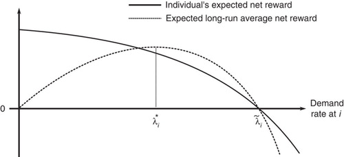
It is worth noting that the theory of non-atomic routing games (see Roughgarden, 2005) assures us that the equilibrium and socially optimal policies both exist and are unique. This allows a simple argument to be formed in order to show that the sum of the joining rates at the individual facilities under a socially optimal policy (let us denote this by η*) cannot possibly exceed the corresponding sum under an equilibrium policy (denoted . Indeed, it is clear that if the system demand rate λ is sufficiently large, then the selfishly and socially optimal joining rates at any individual facility i will attain their ‘ideal’ values and λ*_i (as depicted in Figure 4), respectively, and so in this case it follows trivially that . On the other hand, suppose that λ is not large enough to permit w_i(λ_i)=0 for all facilities i. In this case, w_i(λ_i) must be strictly positive for some facility i, and therefore the probability of a customer balking under an equilibrium strategy is zero (since balking is unfavourable in comparison to joining facility i). Hence, one has in this case, and since η* is also bounded above by λ the result follows.

The conclusion of this section is that, while the ‘containment’ property of observable systems proved in Section 3 does not have an exact analogue in the unobservable case, the general principle that selfish customers create ‘busier’ systems still persists (albeit in a slightly different guise).

5. Heterogeneous customers

An advantage of the anticipatory reward formulation in (3) is that it enables the results from Section 3 to be extended to a scenario involving heterogeneous customers without a re-description of the state space S being required. Suppose we have M⩾2 customer classes, and customers of the ith class arrive in the system via their own independent Poisson process with demand rate λ_i (i=1, 2, .., M). In this case we assume, without loss of generality, that ∑_iλ_i+∑_jc_jμ_j=1. For convenience we will define λ:=∑_iλ_i as the total demand rate. We allow the holding costs and fixed rewards in our model (but not the service rates) to depend on these customer classes; that is, the fixed reward for serving a customer of class i at facility j is now α_ij, and the holding cost (per unit time) is β_ij. Various physical interpretations of this model are possible; for example, suppose we have a healthcare system in which patients arrive from various different geographical locations. Then the parameters α_ij and β_ij may be configured according to the distance of service provider j from region i (among other factors), so that patients’ commuting costs are taken into account.

Suppose we wanted to use a ‘real-time’ reward formulation, similar to (1), for the reward r(⋅) in our extended model. Then the system state would need to include information about the classes of customers in service at each facility, and also the total number of customers of each class waiting in each queue. However, using an ‘anticipatory’ reward formulation, we can allow the state space representation to be the same as before; that is, , where x_j is simply the number of customers present (irrespective of class) at facility j, for j=1, 2, …, N. On the other hand, the set of actions A available at each state x∈S has a more complicated representation. We now define A as follows:

That is, the action a is a vector which prescribes, for each customer class i∈{1, 2, …, M}, the destination a_i of any customer of class i who arrives at the present epoch of time, with the system having been uniformized so that it evolves in discrete time steps of size Δ=(∑_iλ_i+∑_jc_jμ_j)⁻¹. The reward for taking action a∈A at state x is then:

where a_i is the i^th component of a, and:

for i=1, 2 …, M. We note that expanding the action set in this manner is not the only possible way of formulating our new model (with heterogeneous customers) as an MDP, but it is the natural extension of the formulation adopted in the previous section. An alternative approach would be to augment the state space so that information about the class of the most recent customer to arrive is included in the state description; actions would then need to be chosen only at arrival epochs, and these actions would simply be integers in the set {0, 1, …, N} as opposed to vectors (see Puterman, 1994, p 568) for an example involving admission control in an M/M/1 queue). By keeping the state space S unchanged, however, we are able to show that the results of Section 3 can be generalized very easily.

Under our new formulation, the discount optimality equations (using the anticipatory reward functions ) are as follows:

Note that the maximization in (28) can be carried out in a componentwise fashion, so that instead of having to find the maximizer among all vectors a in A (of which the total number is (N+1)^M), we can simply find, for each customer class i∈M, the ‘marginal’ action a_i which maximizes . This can be exploited in the implementation of dynamic programming algorithms (eg, value iteration), so that computation times increase only in proportion to the number of customer classes M.

As before, we define the selfishly optimal policy to be the policy under which the action chosen for each customer arriving in the system is the action which maximizes (obviously this action now depends on the customer class). A selfish customer of class i accepts service at facility j if and only if, prior to joining, the number x_j of customers at facility j, satisfies x_j⩽b_ij, where:

Consequently, under steady-state conditions, the number of customers present at facility j is bounded above by max_ib_ij. It follows that we now have the following definition for the selfishly optimal state space :

Example 2

• We modify Example 1 from earlier so that there are now two classes of customer, with demand rates λ₁=12 and λ₂=10 respectively. The first class has the same cost and reward parameters as in Example 1; that is, β₁₁=3, α₁₁=1 (for the first facility) and β₁₂=3, α₁₂=3 (for the second facility). The second class of customer has steeper holding costs and a much greater value of service at the second facility: β₂₁=β₂₂=5, α₂₁=1, α₂₂=12. Both facilities have two service channels and the service rates μ₁=5 and μ₂=1 remain independent of customer class. We take Δ=(∑_iλ_i+∑_jc_jμ_j)⁻¹=1/34 to uniformize the system.

  We have previously seen that customers of the first class acting selfishly will cause the system state to remain within a set of 12 states under steady-state conditions, withx₁⩽3 andx₂⩽2 at all times. The incorporation of a second class of customer has no effect on the selfish decisions made by the first class of customer, so (as shown in Figure 5) these decisions remain the same as shown in Figure 3 previously. The first table in Figure 5 shows that selfish customers of the second class are unwilling to join the first facility whenx₁⩾2; however, under certain states they will choose to join the second facility whenx₂=3 (but never when x₂>3). As a result, the selfish state spaceis expanded from 12 states to 20.

  Figure 5 Selfishly and socially optimal policies for Example 2.

  Note: At each state x=(x₁, x₂), the corresponding decision vector a=(a₁, a₂) is shown.

  

  Figure 5 shows that the new selfish state spacemay be represented diagrammatically as the smallest rectangle which encompasses bothand, where (for i=1, 2) we have defined:

  It is somewhat interesting to observe thatincludes states in the ‘intersection of complements’. These states would not occur (under steady-state conditions) if the system operated with only a single class of customer of either type, but theydooccur with both customer types present.

  The policy θ* depicted in the second table in Figure 5 has been obtained using value iteration, and illustrates the containment property for systems with heterogeneous customer classes. It may easily be seen that the socially optimal state spaceconsists of only 9 states; under steady-state conditions, the system will remain within this smaller class of states. We also observe that, unlike the selfish decisions, the socially optimal decisions for a particular class of customerareaffected by the decisions made by the other class of customer (as can be seen, in the case of the first customer class, by direct comparison with Figure 3 from Example 1). Indeed, underθ*, customers of the first class never join Facility 2, and customers of the second class never join Facility 1.

It can be verified that the results of Lemmas 2–5, Theorems 1–2 and Lemma 6 apply to the model with heterogeneous customers, with only small modifications required to the proofs. For example, in Lemma 3 we prove the inequality by showing that, for all classes i∈{1, 2,…, M} and facilities j∈{1, 2, …, N}, we have:

for all . In Lemma 4, we can define α_max=max_i,jα_ij and establish a lower bound for similar to (22) by writing and instead of and respectively (so that the action at state 0^j+ is the zero vector 0, ie all customer classes balk); the rest of the inductive proof goes through using similar adjustments. Theorem 2 holds because if was not contained in , then the discount optimality equations would imply, for some i∈{1, 2, …, M} and j∈{1, 2, …, N}:

with , thus contradicting the result of (the modified) Lemma 3. The sample path argument in Lemma 6 can be applied to a customer of any class, with only trivial adjustments needed.

6. Conclusions

The principle that selfish users create busier systems is well-observed in the literature on behavioural queueing theory. While this principle is interesting in itself, we also believe that it has the potential to be utilized much more widely in applications. As we have demonstrated, the search for a socially optimal policy may be greatly simplified by reducing the search space according to the bounds of the corresponding ‘selfish’ policy, so that the methods of dynamic programming can be more easily employed.

Our results in this paper hold for an arbitrary number of facilities N, and (in addition) the results in Section 5 hold for an arbitrary number of customer classes M. This lack of restriction makes the results powerful from a theoretical point of view, but we must also point out that in practice, the ‘curse of dimensionality’ often prohibits the exact computation of optimal policies in large-scale systems, even when the state space can be assumed finite. This problem could be partially addressed if certain structural properties (eg monotonicity properties) of socially optimal policies could be proved with the same level of generality as our ‘containment’ results. It can be shown trivially that selfish policies are monotonic in various respects (eg, balking at the state x implies balking at state x^j+, for any facility j) and, indeed, the optimality of monotone policies is a popular theme in the literature, although in our experience these properties are usually not trivial to prove for an arbitrary number of facilities. In future work, we intend to investigate how the search for socially optimal policies can be further simplified by exploiting their theoretical structure.