Discussion of ‘Accounting for intangible assets: suggested solutions’

1. Introduction

Accounting researchers are sometimes criticised for focusing too much on empirical research of limited relevance to preparers, capital providers or standard setters; however, making conceptual progress is hard – both practitioners and academics will then question whether your contributions are genuinely new. I find the approach adopted by Barker, Lennard, Penman and Teixeira (Barker et al. 2021, referred to as BLPT in this commentary) commendable in that they address core accounting issues in a way that is directly relevant to standard setters. I agree with BLPT that normative accounting research is relatively underdeveloped, and that empirical research is constrained by accounting practice. In my discussion below, I focus on three areas: (1) single project vs. portfolios, (2) internally generated vs. purchased assets and (3) measurement after recognition.

2. Single project vs. portfolios

The arguments put forward by BLPT are often exemplified by reference to research and development (R&D) activities, where the uncertainty is often very high, but the purpose is clearly to develop intangible assets – R&D investments are presumably expected by firms to generate positive net present values regardless of the accounting treatment. Standard setters, including the International Accounting Standards Board (IASB), tend to focus on separate items, transactions and events. In the context of R&D activities, this implies that each project will be evaluated separately and, in the case of IAS 38 – Intangible Assets, divided into a research phase (costs initially recognised as expenses) and a development phase (costs initially recognised as an asset if a set of criteria are met, otherwise the costs are expensed as incurred). In accordance with the focus of standard setters, BLPT adopt a single-project view in their main argumentation. In particular, it is the difficulty of separating out the investment component from transactions that forces the expensing solution: if intangibles are largely in joint expenditures (both current and investment-related), the issue of capitalisation is mute, BLPT argue.

It is natural for a standard setter to develop standards that apply at the transaction level; however, for the purpose of conceptual development, it is worthwhile to extend the discussion to the portfolio level. Consider, BLPT suggest, the outcomes to R&D investment into one medicine in a bio-tech start-up to be highly uncertain, while that in a mature pharmaceutical firm with a portfolio of other medicines being developed is less so. Portfolios of investments diversify and reduce risk, and this may be considered when developing an accounting solution for R&D investments. The mature pharmaceutical firm is a useful example. In my opinion, viewing the portfolio of R&D projects within each particular medical treatment area (e.g. oncology medicines, cardiovascular medicines, gastrointestinal medicines) as the unit of account, and the uncertainty associated with it, would make sense as this would seem to correspond more closely to the business model (rather than treating each R&D project and related transactions separately when applying the standard). There is a parallel here with the so-called area of interest method applied to mining activities, where the unit of account is referred to as a geological area.¹

These considerations aside, BLPT note that the separability problem remains also with a portfolio approach: the asset component cannot be identified when it is embedded in transactions also involving current expenses. BLPT argue that if a pharmaceutical company runs 100 R&D projects but only succeeds in 1 case and fails in 99, recognition of the R&D expenditure as an asset would lead to immediate impairment as implied by rational expectations theory. However, there is clearly an asset component of these investments and, for a portfolio of projects, the expected value of future economic benefits is positive. It may be useful here to compare with the accounting treatment of large populations of obligations with a low probability of realisation, e.g. product warranties. Even though very few of the products fail and trigger warranty payments to customers, a provision for future warranty costs will be recognised and measured at the expected value.² Arguably, a corresponding view on R&D portfolios could be seen as a way to separate the asset component.

BLPT argue that the recognition of an asset must be accompanied by an assessment of the implications for earnings which conveys value from using assets jointly. There will be a certain degree of mismatching in the income statement both when initially recognising investments as expenses and as assets. This points at another aspect of accounting for project portfolios rather than single projects. Using again the example of a mature pharmaceutical company, diversification may take place within and across medical areas, but also over time so that the company has projects in all phases of the medicine lifecycle.

Figure 1 shows a schematic illustration of the cash flow pattern of a successful pharmaceutical product project received some years ago from a financial manager in a large pharmaceutical company. The company strives for a balanced portfolio of projects in terms of having a pipeline of projects in each phase of R&D process (pre-clinical and clinical phases I, II and III), projects in the launch phase where medical doctors must be convinced to start prescribing the new drug, and projects in various stages of the sales phase. According to this illustration, significant cash spending is needed during the launch phase, whereas little marketing is needed at the end of the cycle (large net cash inflows).

Figure 1. Schematic illustration of the cash flow pattern for a (successful) pharmaceutical product project.

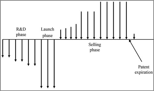
The idea of investing in a balanced portfolio of projects is well established among accountants and it has certain important properties. In particular, for the no-growth case, reported earnings for the balanced portfolio will be the same regardless of whether the investments are initially expensed or capitalised and amortised (the amount expensed will equal the amortisation). BLPT refer to this as the cancelling error property of accounting.³ This property of a balanced portfolio, compared with a single project, is worth considering for standard setters. There are already situations where balance sheet items are measured at an aggregate level, e.g. portfolios of financial assets (IFRS 9 – Financial Instruments), provisions involving a large population of items (IAS 37), and retail inventory (IAS 2 – Inventories). It seems like an unwarranted restriction (overly conservative) to view all investments in internally developed intangibles as single projects conducted in isolation, which is how the current standard (IAS 38) is designed.

Figure 2 presents the income statement for the mature pharmaceutical company AstraZeneca (AZ) during the period 2003–2006 (IFRS 2004–2006, UK GAAP for 2003). AZ operates full-cycle pharmaceutical product projects and has, in expectation, normally a balanced portfolio of projects. According to the annual report notes on intangible assets, no costs related to internally developed product-, marketing-, or distribution rights were capitalised during 2003–2006. In the CEO’s review for 2006, he points at high sales growth and having eleven medicines with sales of more than USD 1 billion; however, he also refers to the need to strengthen the R&D pipeline as the newly approved medicine Exanta had to be withdrawn in the beginning of the year and the medicine Galida had to be stopped at a late stage of development. Also, in 2004–2005, there were problems with Exanta not being approved by authorities, the R&D results for the medicine Iressa not being significant, and a public dispute regarding the medicine Crestor. How does this correspond with the impressive development of operating margins in AZ, from 21% in 2003 to 31% in 2006? Arguably, it is largely the result of a previously balanced portfolio becoming unbalanced.

Figure 2. AstraZeneca’s income statement structure during 2003–2006.

Note. The financial information is based on AstraZeneca’s annual reports for 2004, 2005 and 2006.

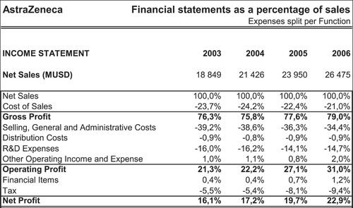
As AZ initially expenses all its R&D costs for internally developed medicines, current sales relate to R&D and selling costs expensed in earlier years, while this year’s R&D and selling expenses primarily relate to future sales. Cost of sales and distribution costs are properly matched. During 2003–2006, there are increased sales from blockbuster drugs developed in the past, while the failure of projects in late R&D phases reduces R&D expenses and planned launch expenses (selling expenses). The improved margin effect is of course only temporary. In a few years’ time, sales will decrease as patents expire (e.g. for the medicine Nexium). AZ actually made a major acquisition in June 2007 (MedImmune) to bridge the expected sales gap caused by the earlier R&D setbacks.

What can we learn from this example? Arguably, AZ strives to have a balanced portfolio of projects which implies that even though the company initially expenses all R&D and launch cost investments, this is not likely to significantly distort the income statement. BLPT concludes in this context (Appendix 1): ‘[…] in a mature brand or pharmaceutical companies where advertising or R&D is roughly a constant percent of revenue, there is little issue in the accounting for intangible assets.’ However, the AZ example shows that when a balanced portfolio turns unbalanced due to failed projects, the effects caused by initially expensing all R&D and launch costs create different effects compared to if the investments had been initially capitalised. Arguably, the increasing earnings and operating margins following the project failures will be difficult to interpret by investors. Capitalisation of such expenditures would instead have triggered impairments as the projects failed, which would, arguably, make more sense following project failures.

Another relevant aspect concerns the internal use of accounting information for management control purposes. Even though immediate expensing and capitalisation with amortisation generates the same earnings numbers for a balanced R&D project portfolio with no growth, the initial expensing of all investments causes a disconnection between current sales and current R&D expenses and much of the current selling expenses, that will make it difficult to evaluate performance internally and to make business decisions. Returns and product margins will be difficult to measure and R&D and launch activities may be perceived as sunk cost instead of investments. I recently learned from a listed technology company with significant annual R&D investments that only the projects that are capitalised under IAS 38 are subject to separate approval by the board of directors. For these projects, there must therefore be financial projections and calculations available. This is also necessary as there will be a need to perform impairment tests in later periods. R&D projects that are not capitalised are not financially evaluated in the same way. It may seem odd that the recognition criteria in IAS 38 are influencing internal project evaluation and decision-making in this way. Perhaps a potential advantage of capitalising costs related to intangible assets is that such investments are then evaluated more rigorously by companies?

3. Internally generated versus acquired intangibles

IAS 38 distinguishes between separate acquisition, acquisition as part of a business combination, and internally generated intangible assets. Separately acquired intangible assets will initially be recognised as assets, as the probability criterion is always considered to be satisfied (IAS 38, p. 25) and as costs can usually be measured reliably (p. 26). For intangible assets acquired as part of a business combination, the probability and reliable measurement criteria are also always considered to be met (p. 33). BLPT argue that capitalisation of intangible assets where there is high uncertainty will result in mismatching due to frequent impairments which, in turn, destroys information in earnings about future cash flows. BLPT note, however, that there is one case where income statement errors are minimised because the asset is not expected to lose value (amortisation) and the likelihood of impairment is very low, namely for land, purchased goodwill and indefinite-lived intangibles in an acquisition. In my opinion, referring here to the intangible assets, this low likelihood of impairment is not because of low uncertainty about the realisation of future cash flow from these assets, but rather the political process that led to the abolishment of goodwill amortisation (Ramanna 2008, Zeff 2010) and built-in deficiencies in the design of the IAS 36 (Impairment of Assets) impairment test (Johansson et al. 2016). This brings us to the issue of internally generated assets vs. purchased ready-made assets.

Many successful companies are good at innovation and organic growth, involving internal generation of intangible assets. Yet, purchases of ready-made assets are initially recognised as assets while internally generated assets are to a great extent initially expensed. Barker and Penman (2018, p. 342) refer to this as an anomaly – an acquisition may not in itself make the expected economic benefits from an asset less uncertain. In a somewhat similar vein, Lev (2018, p. 475, emphasis added) argues: ‘[…] expensing internally generated intangible investments, while capitalising the functionally identical acquired intangibles […] decreases substantially the usefulness of reported earnings […]’. Both BLPT and Barker and Penman (2018) emphasise that there is a threshold before investments in internally developed intangibles can be recognised as assets: it must be possible to establish a reliable ex ante amortisation schedule that results in low ex post mismatching errors. This involves a problem of timing that will be addressed by using an example.

Figure 3 shows a numerical example with two scenarios for a company investing in a new brand. In scenario A, the company develops the brand internally by investing 1000 in sales and promotion (S&P) costs at the end of the year 0, 1, 2, 3 and 4. Each investment generates sales in the coming year and at the end of year 5 the brand-building is completed. From this point forward, the company invests 500 per year to maintain the brand with no growth in sales. The last investment of 500 is made at the end of year 9, and at the end of year 10, the brand is terminated. In scenario B, the company waits 5 years and then acquires an identical ready-made brand as in scenario A, at the end of year 5 for 3014. The same conditions as in scenario A applies during year 6–10. In scenario A, all S&P costs are expensed as incurred, while in scenario B, the acquisition of the brand is linearly amortised over 5 years. The internal rate of return is the same for both scenarios (approximately 9.39%).

Figure 3. Illustrative example: internally developed vs. acquired intangible asset.

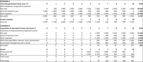
The example aims to point at the problem of difference in timing between internally developed and acquired assets. The existing brand assets at the end of year 5 are identical in scenarios A and B and the expected economic benefits from the asset in scenario A are not less uncertain than from the asset in scenario B. However, the uncertainty in scenario A is gradually reduced as the brand is developed during years 1–5 and only at the end of year 5, BLPT’s threshold of a reliable amortisation pattern is fulfilled and the purchased brand in scenario B can therefore be capitalised. Before the amortisation threshold is met, there is no recognisable asset according to BLPT and Barker and Penman (2018) and then suddenly there is one at the end of year 5. However, in scenario A, no asset may be recognised because the accounting is not prepared retrospectively with hindsight. The example illustrates that, because of differences in the timing of uncertainty evaluations, internally developed and acquired intangibles are not directly comparable. This is not satisfactory, but it would seem some retrospective mechanism is required to address the problem. BLPT offer some paths towards possible solutions to this problem in their section on ‘conditional capitalisation’. I provide some further comments on this in the next section.

BLPT point at the need to strike a balance between when to initially expense, and when to capitalise, investments in intangible assets. Although both create mismatching problems, my perception is that BLPT fear excessive capitalisation more than early expense recognition. However, there is also a development of selective use of accounting information that should be acknowledged in this context. In Figure 3, the organic growth scenario (A) generates a higher total net profit compared to acquiring the ready-made brand (scenario B).⁴ However, if the EBITA measure is used instead, disregarding amortisation, the total profit is higher for scenario B. Over time, I believe IFRS Standards are increasingly favouring acquired growth over organic growth. One reason for this is the absence of amortisation of purchased goodwill and intangibles with indefinite lives, and a low probability of impairment due to the design of the impairment test (Johansson et al., 2016), which implies that the impact of an acquisition on the post-acquisition operating profit becomes largely independent of the price level paid.⁵ In addition, for intangibles that are amortised, and when there is impairment of intangibles, these expenses will be disregarded by measures such as ‘adjusted EBITA’,⁶ commonly used by firms and analysts. The IASB opened up for the use of such measures in IFRS 8 – Operating Segments and the recent Discussion Paper on Business Combinations (IASB 2020) offers firms to use more customised measures when reporting on acquisitions. Thus, even if IAS 38 is, in the future, revised and improved in terms of striking a better balance between capitalisation and immediate expensing, it may not make any difference to users. If investors and analysts choose to systematically disregard all amortisation and impairment losses by monitoring ‘adjusted EBITA’ numbers, firms will have a strong incentive to primarily purchase ready-made intangibles and to make corporate acquisitions.

4. Measurement after recognition

BLPT note that subsequent measurement is essentially the same in IAS 16 – Property, Plant and Equipment and IAS 38, for example, the definitions of useful life are identical. BLPT emphasise that capitalisation requires that a reliable ex ante amortisation pattern can be established and argue that for less certain assets, such as R&D, amortisation is likely to introduce severe mismatching. It is worthwhile here to consider the IAS 38 formulation (p. 97, emphasis added):

The amortisation method used shall reflect the pattern in which the asset’s future economic benefits are expected to be consumed by the entity. If the pattern cannot be determined reliably, the straight-line method shall be used.

It would seem like the formulation in IAS 38 goes against the BLPT view, i.e. if the amortisation pattern cannot be reliably determined, the investment should be initially expensed according to BLPT, not capitalised and amortised linearly. As referred to earlier, for a diversified and balanced R&D project portfolio in the pharmaceutical industry, there is a positive expected value of future cash flows, there is prior knowledge of the cash flow patterns from previously developed pharmaceuticals and there is an expiration date for the patent that can be used to determine useful life. If such an asset is recognised on the balance sheet, it would seem like an amortisation schedule would best be determined based on the development of the present value of remaining cash flows expected to be received (economic depreciation). Accordingly, the formulation in IAS 16, where there is no preference for any particular depreciation method (p. 62), would seem to make more sense also for intangible assets.⁷ As advocated by BLPT, Boeing’s application of US GAAP offers interesting routes forward, as Boeing does not separate tangible from intangible development costs, views the development efforts at an aggregate programme level and applies the units of production method for amortisation/depreciation.

As regards subsequent measurement, I believe the matters covered by BLPT could be extended to include the treatment of subsequent costs more comprehensively. In IAS 16, a distinction is made between subsequent costs that are to be expensed as incurred and those that shall be capitalised. Before the revision of IAS 16 in 2003, the so-called maintain/enhance approach was applied to subsequent costs (capitalise only when the asset is enhanced), however, the IASB found that in practice it was difficult to make this distinction as some expenditures seem to both maintain and enhance (IAS 16, BC5). Instead, a components approach is prescribed, where replacements of asset components are capitalised (IAS 16, p. 13). For intangible assets, it would seem like they often consist of ‘base assets’ (e.g. trademarks, recipes, software, patents) where there are costs to maintain these assets (e.g. advertising, R&D), but also new investments made to enhance them (e.g. upgrades of software, brand expansion to new products). This is not, however, the view put forward in IAS 38.

IAS 38 does not have a general section on subsequent costs; however, the standard says that the general recognition criteria (p. 18, emphasis added) ‘[…] apply to costs incurred initially to acquire or internally develop an intangible asset and those incurred subsequently to add to, replace part of, or service it.’ The implications are set out in some detail in p. 20 (emphasis added):

The nature of intangible assets is such that, in many cases, there are no additions to such an asset or replacements of part of it. Accordingly, most subsequent expenditures are likely to maintain the expected future economic benefits embodied in an existing intangible asset rather than meet the definition of an intangible asset and the recognition criteria in this Standard. In addition, it is often difficult to attribute subsequent expenditure directly to a particular intangible asset rather than to the business as a whole. […] Consistently with paragraph 63, subsequent expenditure on brands, mastheads, publishing titles, customer lists and items similar in substance (whether externally acquired or internally generated) is always recognised in profit or loss as incurred.

As discussed by BLPT, there is a restriction of assets to ‘rights’ in the new IASB Conceptual Framework. A right can meet the definition of an economic resource, and hence be an asset, even if the probability of generating future economic benefits is low. This opens up for a view where an intangible base asset may exist rather early in the R&D process (e.g. approved patents for critical molecules of a new drug) that may be conditionally capitalised awaiting regulatory approval of the medicine. Some years ago, an IASB working group on extractive activities, suggested a solution along similar lines of thought. The IASB (2010b) proposal suggests the use of the area of interest method for determining the unit of account and an asset recognition model based on acquired legal rights of exploration. Subsequent costs for exploration, evaluation and development would be capitalised as ‘enhancements of the legal rights’ as they do not represent separate assets but are necessary in order to obtain future economic benefits (IASB 2010b, p. 53, Gray et al. 2019, p. 51).

5. Closing remarks

The article by Barker, Lennard, Penman and Teixeira highlights the need for the IASB to reconsider its view on accounting for intangibles in IAS 38. In doing so, the authors point at the need for future regulation to safeguard a low level of distortion of the income statement. Fundamental issues must be addressed, such as the difference (if any) between tangible and intangible assets and how to deal with uncertainty about investment outcomes to adequately balance current and future mismatching errors. As discussed in the article and in this commentary, this may involve, for example, more conditional capitalisation and more of a portfolio perspective on investment in intangibles. This is an urgent matter as the IAS 38 constraints make organic growth look increasingly expensive compared to the costs of acquiring intangibles through business combination that are either not recognised in the income statement, due to ineffective goodwill impairment tests, or disregarded due to the use of EBITA and similar measures.

Disclosure statement

No potential conflict of interest was reported by the author(s).

Notes

1 In a mining industry review, PwC (2012, p. 21) states:

After recognition has been deemed appropriate, an entity must determine the ‘unit’ to which exploration and evaluation expenditures should be allocated. The most common approach in the mining industry is to allocate costs between areas of interest. This involves identifying the different geological areas that are being examined and tracking separately the costs incurred for each area. An area of interest normally contracts in size over time as work progresses towards the identification of individual mineral deposits.

2 More general use of expected value was suggested for non-financial liabilities in the 2005 exposure draft regarding amendments to IAS 37 – Provisions, Contingent Liabilities and Contingent Assets (IASB 2005, p. 16). BLPT refers to rational expectations theory when arguing in favour of expense recognition in a case where the most likely outcome is failure (99 out of 100 cases fail). For liabilities, however, such rationality has been questioned (IASB 2010a, p. 18):

The term ‘best estimate’ is ambiguous. Accountants often use it to mean ‘most likely outcome’. However, [IAS 37] describes it as ‘the amount that an entity would rationally pay to settle the obligation at the end of the reporting period or to transfer it to a third party at that time’. Rationally, an entity would pay an amount that is not based solely on the most likely outcome. Rather, it would pay an amount that reflects the probability-weighted average of all possible outcomes. This amount is known as the ‘expected value’ of the outflows.

3 The properties of counterbalancing errors for balanced portfolios of projects are described by Johansson and Östman (1995). They also evaluate the relationship between growth in R&D expenditure, growth in the capitalised R&D asset and the method of depreciation.

4 Scenario A has several years with negative cash flows in the beginning that are discounted relatively few years. To compensate for these early negative years, having also more years of discounting in the later periods, high surpluses are needed to generate the same IRR as in scenario B.

5 The difference between goodwill and other intangible assets with indefinite useful lives should, however, be acknowledged; the useful life of the latter category will be assessed each period and there will be a change to finite useful life if the indefinite useful life assessment is no longer supported (IAS 38, p. 109).

6 ‘EBITA’ refers to earnings before interest, taxes and amortisation. ‘Adjusted’ refers to the exclusion of non-recurring items such as impairment losses.

7 IAS 16 (p. 62):

A variety of depreciation methods can be used to allocate the depreciable amount of an asset on a systematic basis over its useful life. These methods include the straight-line method, the diminishing balance method and the units of production method.

References

- Barker, R., Lennard, A., Penman, S.H., and Teixeira, A, 2021. Accounting for intangible assets: suggested solutions. Accounting and Business Research, doi:10.1080/00014788.2021.1938963.
- Barker, R., and Penman, S.H, 2018. Moving the conceptual framework forward: accounting for uncertainty. Contemporary Accounting Research, 37 (1), 322–357.
- Gray, S.J., Hellman, N., and Ivanova, M.N, 2019. Extractive industries reporting: a review of accounting challenges and the research literature. Abacus, 55 (1), 42–91.
- IASB, 2005. Exposure Draft of Proposed Amendments to IAS 37 Provisions, Contingent Liabilities and Contingent Assets and IAS 19 Employee Benefits. June 2005. London: International Accounting Standards Board.
- IASB, 2010a. Measurement of Liabilities in IAS 37: Proposed Amendments to IAS 37. Exposure Draft 2010/1. London: International Accounting Standards Board.
- IASB, 2010b. Extractive Activities. Discussion Paper DP/2010/1. London: International Accounting Standards Board.
- IASB, 2020. Business Combinations – Disclosures, Goodwill and Impairment. Discussion Paper DP/2020/1. London: International Accounting Standards Board.
- Johansson, S.-E., Hjelström, T., and Hellman, N., 2016. Accounting for goodwill under IFRS: a critical analysis. Journal of International Accounting, Auditing & Taxation, 27, 13–25.
- Johansson, S.-E., and Östman, L., 1995. Accounting Theory: Integrating Behaviour and Measurement. London: Pitman Publishing.
- Lev, B, 2018. The deteriorating usefulness of financial report information and how to reverse it. Accounting and Business Research, 48 (5), 465–493.
- PwC, 2012. Financial Reporting in the Mining Industry. International Financial Reporting Standards. London: PricewaterhouseCoopers.
- Ramanna, K, 2008. The implications of unverifiable fair-value accounting: evidence from the political economy of goodwill accounting? Journal of Accounting and Economics, 45 (2008), 253–281.
- Zeff, S.A, 2010. Political lobbying on accounting standards – US, UK, and international experience. In Comparative International Accounting, by C. Nobes, and R. Parker, Chap. 11, 11th edition. Harlow, Essex, U.K.: Pearson.