Using Variance Structure to Quantify Responses to Perturbation in Fish Catches

Abstract

We present a case study evaluation of gill-net catches of Walleye Sander vitreus to assess potential effects of large-scale changes in Oneida Lake, New York, including the disruption of trophic interactions by double-crested cormorants Phalacrocorax auritus and invasive dreissenid mussels. We used the empirical long-term gill-net time series and a negative binomial linear mixed model to partition the variability in catches into spatial and coherent temporal variance components, hypothesizing that variance partitioning can help quantify spatiotemporal variability and determine whether variance structure differs before and after large-scale perturbations. We found that the mean catch and the total variability of catches decreased following perturbation but that not all sampling locations responded in a consistent manner. There was also evidence of some spatial homogenization concurrent with a restructuring of the relative productivity of individual sites. Specifically, offshore sites generally became more productive following the estimated break point in the gill-net time series. These results provide support for the idea that variance structure is responsive to large-scale perturbations; therefore, variance components have potential utility as statistical indicators of response to a changing environment more broadly. The modeling approach described herein is flexible and would be transferable to other systems and metrics. For example, variance partitioning could be used to examine responses to alternative management regimes, to compare variability across physiographic regions, and to describe differences among climate zones. Understanding how individual variance components respond to perturbation may yield finer-scale insights into ecological shifts than focusing on patterns in the mean responses or total variability alone.

Received July 26, 2016; accepted February 28, 2017 Published online April 25, 2017

Perturbation due to anthropogenic or natural forces can disrupt stable ecosystem conditions. Understanding how ecological systems respond to large-scale perturbations, both gradual and abrupt, has important implications for the management and monitoring of natural resources. Ecological systems include dynamic networks of complex interactions within which organisms vary over space and time, but in far more complex ways than independent deviations from a constant mean. Although variability has often been viewed as something to minimize through adequate sampling, it may also provide valuable information about ecological processes (Kratz et al. 1995). Ecosystems are influenced by many drivers (Scheffer et al. 2001), which can induce changes in an ecosystem state rapidly (e.g., invasive species) or more gradually over a longer period of time (e.g., climate change). The ways in which a system responds to perturbations depend on complex interactions between physical (e.g., climate and hydrology) and biological processes (e.g., demographic and trophic processes). In resilient systems, there is a high capacity to reorganize after a disturbance, such that the state-space remains essentially unchanged; in less resilient systems, however, the organization following disturbance can differ substantially from the predisturbance state. State-space can be defined as the function, structure, identity, and feedbacks that characterize an ecosystem state (Walker et al. 2004). It is important to understand reorganizations because they may be undesirable relative to conservation goals, management objectives, and socioeconomic dynamics.

The idea that perturbation elicits a response in the variability of a state variable was set forth by Odum et al. (1979), who defined an ecosystem perturbation as “any deviation, or displacement, from the ‘nominal state’ in structure or function at any level of organization. The nominal state is the normal operating range, including expected variance.” In recent decades, attention has been paid to the identification of generalizable indicators (e.g., changes in the mean, variance, and skewness of variables, including pollutants, climatic moisture, greenhouse gases, and chlorophyll) to detect and even predict major ecological shifts (Brock and Carpenter 2006; Scheffer et al. 2009; Carpenter et al. 2011).

We propose that shifting variance structure can be used as an indicator of perturbation-induced ecological reorganization. Partitioning total variability into dominant source components (e.g., spatial and temporal) may provide quantifiable indicators of population-level responses associated with major ecosystem shifts and on time scales relevant to the monitoring and management of fishery resources. Changes in variance structure may even indicate cascading effects of perturbations through a food web (e.g., via species interactions). Similarly, Underwood (1991, 1994) proposed using the temporal change in variance as an indicator of perturbation-induced change, although his proposed approach was flawed because the variance estimates in his tests combine systematic and chance temporal variation, sampling error, and autocorrelation (Stewart-Oaten and Bence 2001). Variance partitioning allows variability to be partitioned into component sources, such as spatial (site to site), coherent temporal (year to year), ephemeral temporal (site × year), trend, and observational error (VanLeeuwen et al. 1996; Urquhart et al. 1998; Wagner et al. 2013). Irwin et al. (2013) applied such a variance partitioning framework to fish count data, quantifying the contribution of each component using a negative binomial mixed modeling approach. If it can be shown that the source components of variability are sensitive to how populations respond to ecological shifts, this approach may prove valuable by identifying or improving measurable attributes of responses to large-scale perturbation.

Our objective was to examine whether indirect effects of a large-scale ecological perturbation could be quantified retrospectively by a change in the structure of the variation (e.g., spatial and temporal) in a target population monitored using standardized sampling. We present a case study analysis using long-term monitoring data to explore the idea that an ecological perturbation may induce a shift in a population’s underlying variance structure. Specifically, we analyzed count data from a fishery-independent gill-net survey targeting Walleye Sander vitreus in Oneida Lake, New York. Sustained monitoring of Oneida Lake provides one of the most complete data sets on freshwater fish populations in the world, and data from this system have been used to advance understanding of food webs, fish populations, and fisheries (Forney 1980; Nate et al. 2011; Rudstam et al. 2016b). We chose Oneida Lake because it is a well-studied system that underwent a major ecological shift during the early 1990s, when an increase in the double-crested cormorant Phalacrocorax auritus (hereafter, “cormorant”) population (Coleman et al. 2016) and an invasion of dreissenid mussels (i.e., zebra mussels Dreissena polymorpha and later quagga mussels Dreissena bugensis) occurred. We predicted that these disturbances would be a strong enough perturbation to the ecosystem that their effects would be detectable in the variance structure of time series data produced by fishery-independent surveys. Specifically, we were interested in three questions: (1) Can we detect a statistical signal to support the timing of perceived transitions related to these perturbations? (2) Do the magnitudes and relative contributions of the variance components change in response to perturbation? (3) Is there evidence of spatial reorganization as a result of the perturbations? We used a model-based evaluation with time-period-specific parameters to address these questions.

Methods

Study site

Oneida Lake has the largest surface area (206.7 km²) of any lake entirely inside the borders of New York State, and it supports important recreational fisheries, including one for Walleyes. Major changes to this ecosystem occurred during the early 1990s, including increased cormorant abundance (Rudstam et al. 2004; Irwin et al. 2008a) and the establishment of nonnative dreissenid mussels. The cormorant population increase is largely attributed to reductions in environmental organochlorines (e.g., DDT) and release from human persecution (Weseloh et al. 1995; Rudstam et al. 2004). Acting as a top predator in Oneida Lake, cormorants have exerted strong predation pressure on the fish populations, pressure that in some cases is comparable to that of angler harvest (on adult fish) and even exceeds that of angler harvest (on subadult fish) (VanDeValk et al. 2002; Rudstam et al. 2004; DeBruyne et al. 2013). At about the same time, dreissenid mussels altered the ecosystem through increased water clarity (Secchi depth increased from approximately 2.6 m prior to the invasion to 3.5 m), disruptions to trophic dynamics, and significant habitat modifications (Mayer et al. 2002; Zhu et al. 2006).

The Oneida Lake ecosystem in recent decades has been thought to be fairly distinct from that in the years prior to the major perturbations (Zhu et al. 2006; Irwin et al. 2016). The early 1990s have previously been identified as the approximate break point in the time series associated with the major changes in the lake (Mayer et al. 2000; Irwin et al. 2008b). It should be noted that other ecological changes have likely also had influences on Oneida Lake during the past several decades. For instance, nutrient loadings were reduced following the signing of the Great Lakes Water Quality Agreement in 1972, and invasive White Perch Morone americana and Gizzard Shad Dorosoma cepedianum periodically contribute high production of young (Fitzgerald et al. 2006), which can alter Walleye foraging behavior and potentially their catchability. Angler harvest is also likely to vary over time. Even so, cormorant predation and the presence of dreissenid mussels have been thought to be the major drivers of changes in the lake, including the decline of some fish populations (Coleman et al. 2016; Irwin et al. 2016). For example, the mean densities of Walleyes remained below their historical averages for a number of years following the establishment of dreissenid mussels and increased cormorant abundance during the early 1990s (Rudstam et al. 2004; Irwin et al. 2008a).

Data

We used data from a long-term (1958–2014 [excluding 1974, for which data were unavailable]), fishery-independent survey of Oneida Lake by researchers at Cornell University (Rudstam and Jackson 2015). This is a fixed-site, annual survey conducted with standardized, variable mesh, multifilament gill nets. The sampling gear is comprised of four gangs (i.e., strings of nets) of six 7.6-m panels sewn together, for a total net length of 183 m and a depth of 1.83 m. The mesh sizes within a gang consist of one panel at each of the following stretched mesh sizes: 38, 51, 64, 76, 89, and 102 mm. The gill nets are set around sunset and hauled around 0730 hours. The survey spans the period from June through mid-September, with one site being sampled per week in a standardized sequence, for a total of 15 sites annually. All fish captured in the nets are identified to species and enumerated, resulting in 15 spatially explicit observations of Walleye catch per survey year.

Statistical analyses

We used a negative binomial linear mixed model to evaluate hypotheses as to how variance structure responds to perturbation. The negative binomial distribution was assumed for the response variable because the variability in predicted Walleye catches was greater than the mean (i.e., the data were overdispersed), thereby violating the assumptions of the Poisson distribution. (The negative binomial distribution is an extension of the Poisson distribution with a shape parameter that makes it suitable for overdispersed count data, which are characteristic of ecological survey data.) Parameter estimation was based on the 1958–2014 time series; however, an indicator variable (p) was used to identify years associated with the pre- and postperturbation periods and allow for period-specific parameter estimates. All analyses were performed using AD Model Builder (Fournier et al. 2012) and R (R Development Core Team 2015).

We used a log-link function to determine expected Walleye catch, such that the natural logarithm of the catch (η_tj) in year t at site j was a linear function of the predictors:

where is the period-specific intercept, λ is the fixed slope for a temporal trend using year (t) as the covariate, and a_tp and b_jp are period-specific estimates of the random effects (VanLeeuwen et al. 1996) associated with year and site, respectively. The year covariate was centered on the mean year to improve convergence and increase the interpretability of the intercept parameter. The global trend (λ) was assumed to be influenced by longer-term processes and therefore was estimated as a single parameter applied to the full time series. Random effects provide a way to quantify the effect of a grouping level (year or site) in relation to the mean effect of all groups combined. All random effects were assumed to be independent and identically distributed according to a Gaussian distribution with a mean of 0 and a variance of σ_x², where x represents the distinct random effects (spatial or temporal). Specific parameters were allowed to vary by time period based on our hypothesis that variance structure would be responsive to perturbation, such that the mean and variance components were time-period specific.

The remaining two equations in the model are

where µ_tj is the expected Walleye catch in year t at site j on the original (nonlogarithmic) scale, Y_tj is the observed Walleye catch in year t at site j, and κ_p is the period-specific shape parameter of the negative binomial distribution. In each year, κ determines how much extra (above-Poisson) variation there is among sites through its relationship with μ. The variance of the negative binomial distribution is assumed to be a quadratic function of the mean, with the quadratic term being dependent on the shape parameter, that is,

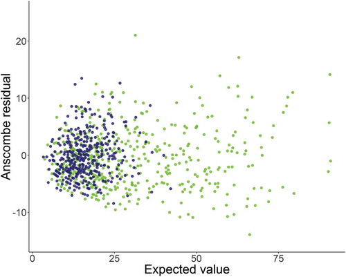
Thus, the relationship of the variation to the mean is allowed to differ between periods. Model fit was evaluated using Anscombe residuals (Anscombe 1953; Hilbe 2011).

Likelihood profiling was used to determine the year in which the change from the pre- to the postperturbation period occurred. We evaluated the above model at every possible change-point year for the available data (i.e., all years except the first and last ones in the time series) using the log-likelihood. All models were equally parsimonious, so that the change point associated with the model with the largest log-likelihood was deemed the most appropriate. Subsequent results are based on the single, optimal change point.

We then used the linear mixed model with the optimal change-point year to evaluate the magnitude and structure of the variability in gill-net catches prior to and following the dreissenid mussel invasion and the cormorant population increase. We compared coherent temporal and spatial variability between periods to evaluate whether the structure of the variability changed after perturbation.

In mixed models, random effects are often used to account for clustering in the data, but they can also offer additional information about the behavior of the individual grouping variables (e.g., sites and years). In this study, we were specifically interested in understanding whether all sites have declined proportionately from historical catch levels or whether there has been a disproportionate shift among sites. A large positive site random effect would indicate that a site contributed more to Walleye catch than average for a particular period, and a large negative random effect would indicate that a site contributed less than average. If there were no changes in the relative contributions of sites following the perturbations, we would not expect a shift in the site random effect rankings even if a decline in the mean response was observed due to lower overall catch rates.

Results

The likelihood profiling indicated that 1989 was the optimal change-point year for separating the gill-net time series into pre- and postperturbation periods. There was a distinct peak in the log-likelihood surrounding the perceived timing (1988–1991) of the ecological shifts in Oneida Lake (Figure 1). The minimum, mean, and maximum annual catches of Walleyes were lower during the later time period. The mean catch was reduced by about 50%, and the maximum catch was about 40% of that in the preperturbation period (Figure 2; Table 1).

TABLE 1. Summary statistics (mean, minimum, maximum, and sample size of Walleye gill-net catches) aggregated across all sites and parameter estimates (SDs in parentheses) from the linear mixed model for the pre- (1958–1988, except for 1974) and postperturbation (1989–2014) periods in Oneida Lake, New York. Slope was not modeled as time-period specific.

Statistic or estimate	Pre	Post
Observed catches
Mean	32	17
Minimum	1	0
Maximum	220	90
Sample size	450	390
Parameter estimates
Fixed effects
Intercept (µ)	3.267 (0.186)	2.709 (0.148)
Slope (λ)	0.002 (0.006)	0.002 (0.006)
Shape parameter (κ)	2.091 (0.155)	2.346 (0.203)
Random effects
Coherent temporal (σa^2)	0.102 (0.039)	0.117 (0.045)
Spatial (σb^2)	0.345 (0.133)	0.096 (0.043)

FIGURE 1. Log-likelihood values of Walleye catch plotted across possible change-point years. The solid black line represents the likelihood profile for the full time series; the colored lines represent likelihood profiles from truncated time series (i.e., with the removal of early and/or late years). The change-point was robust to time series length. The log-likelihood values are not shown along the y-axis owing to scaling differences among the four time series; the peak around 1989 indicates the optimal change point.

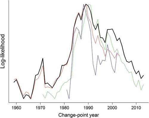
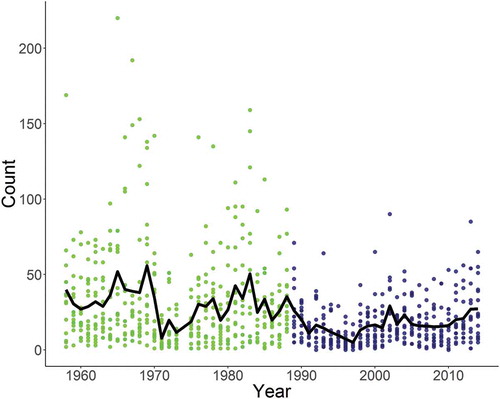
FIGURE 2. Observed Walleye catch by site and year for fifteen fixed sites in Oneida Lake from 1958 to 2014 (data were not available for 1974). The black line represents mean annual catches over time, the green dots represent the catches at individual sites in preperturbation period, and the blue dots represent the catches at the individual sites in the postperturbation period.

Importantly, we also observed a reduction in the variability in catch rates over time, as high catches at individual sites became less frequent (Figure 2). The shape parameter of the negative binomial distribution was slightly higher during the postperturbation period (Table 1), indicating a small reduction in the rate at which the variance in gill-net catches changed with the mean. Thus, in addition to the reduction in the total variability the structure of the variability also changed following 1989, particularly spatial variability (Figure 3; Table 1). The predicted catches from the negative binomial mixed model were in general agreement with the observed data for both the pre- and postperturbation periods (Figure 4). The Anscombe residuals that were used to further evaluate model fit appeared to be approximately normally distributed across the range of the predicted values; there was no indication of extreme outliers (Figure 5).

FIGURE 3. Normal density plots showing the shifts in (A) spatial and (B) temporal variability relative to the period-specific mean catch during the pre- and postperturbation periods (represented by the green and blue areas, respectively).

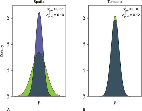
FIGURE 4. Observed (green and blue areas) and predicted (white areas) Walleye catch during (A) the preperturbation period and (B) the postperturbation period. The x-axis represents Walleye catches, aggregated across sites and years, into nine bins with ranges shown. Bar width scales with bin width.

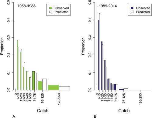
FIGURE 5. Plot of Anscombe residuals based on fitting a negative binomial mixed model to the catches of Walleyes. Green dots depict values from the preperturbation period, blue dots values from the postperturbation period.

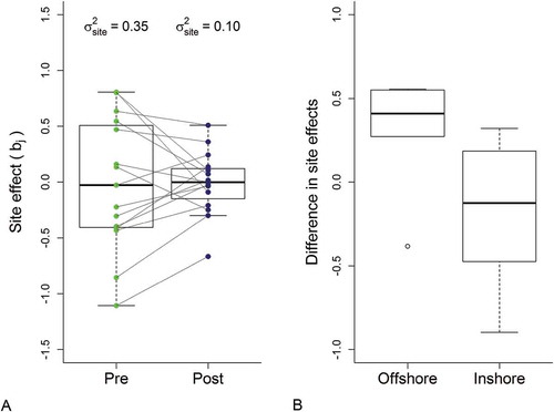
In the model, the maximum likelihood estimate for spatial variability (σ_b²), which was 0.35 in the years prior to the break point, and declined to 0.10 in the postperturbation period (Table 1; Figure 3)—a 72% reduction in the estimated among-site variability. By contrast, the temporal variability remained relatively stable between the two time periods (pre: σ_a² = 0.10; post: σ_a² = 0.12). Additionally, the decline in spatial variability reflected proportionally different relative changes at the different sites, as indicated by the shifting rank order of the site-specific random effects (Figure 6A). The difference between the post- and preperturbation random effects provides a relative measure of the contributions of the individual sites that might help us understand these patterns by pinpointing the relevant site-specific attributes. This analysis, however, was not designed to investigate specific causal mechanisms operating within this system but to investigate the potential for variance structure to serve as a statistical indicator of some complex responses to large-scale perturbation. Purely for illustrative purposes, we performed post hoc analyses to evaluate the site characteristics (i.e., substrate type, depth, and distance from shore) of the survey locations vis-à-vis the difference in spatial random effect values between the pre- and postperturbation time periods. This exploratory analysis indicated that Walleye catches at the inshore sites have generally declined more severely than those at the offshore sites (Figure 6B). The mean catches at the inshore sites (n = 9) all declined following the perturbations, while those at one-third of the offshore sites (n = 6) increased slightly. Even so, some of the highest overall catches continue to come from the inshore sites. Coherent temporal variability (σ_a²) was relatively unchanged between the two time periods (Figure 3) and represented a relatively small component of the total variability during the preperturbation period (about 23%). Due to the decline in spatial variability, however, the estimates of coherent temporal and spatial variability were about equal in the postperturbation period (Table 1).

FIGURE 6. Box plots showing (A) the spread of the individual-site random effects in the pre- and postperturbation periods and (B) the change in site random effects (i.e., postperturbation less preperturbation) for inshore and offshore sites. The boxes represent the interquartile range of the values, with the dark horizontal line indicating the median value, and whiskers extending to the most extreme value within 1.5× the interquartile range. The circles in panel (A) represent individual sites; the lines connect the individual site random effects between the two time periods to show how a site’s rank changed relative to the other sites in terms of catch magnitude.

Discussion

We were able to objectively detect a change point in the time series of Walleye catches that is consistent with the timing of perceived ecological shifts in Oneida Lake (e.g., Mayer et al. 2000; Irwin et al. 2008b, 2016; Coleman et al. 2016) and quantify shifts in the variance structure using a mixed modeling approach. In this lake, there has been a marked decline in gill-net catches of Walleyes over time. Concurrent with the decline in the mean catch of Walleyes, a reduction in the site-to-site variability was observed, suggesting homogenization across sites in terms of relative catches. Additionally, we have shown that the variance structure was time sensitive; therefore, variance partitioning appears to be useful for providing additional, finer-scale information about the responses to ecological shifts—information beyond that provided by the changes in means or total variability.

Disentangling the spatial and temporal components of variability provides information about how a system is changing across space and through time, a property that could be useful for the adaptation of management and monitoring to dynamic ecosystems. For example, random effects could be used to evaluate differential growth rates due to geographic location or gradual shifts over time. Increasing variance has been proposed as a signal associated with the transition between stable states (Brock and Carpenter 2006; Scheffer et al. 2009; Carpenter et al. 2011), but the responsiveness of variance components to large-scale ecological change appears to be a relatively new development (however, see Guttal and Jayaprakash 2009). By decomposing variability into time-varying component sources, we were able to identify spatially explicit changes (e.g., a disproportionate diminishing of high-catch events) beyond those that could have been inferred from the mean response alone. In this study, we were interested in the general behavior of variance structure in response to perturbation; however, this analytical approach could be extended to other investigations, such as examining the responses to alternative management regimes, comparing variability across physiographic regions, and describing differences among climate zones.

Our mixed-modeling approach provided evidence that the sources of variability associated with a response variable can change in relative importance over time and in response to perturbation. In our study, temporal variability remained relatively unchanged, whereas the spatial variance component was reduced by 72%. In addition to the fact that the overall spatial variance parameter was reduced in the latter part of the time series, the individual sampling sites did not respond in a consistent manner. Generally, there was a homogenization across sites toward lower Walleye catches, with a reduction in the spatial patchiness of catch rates and a reorganization of the rankings of the site-level random effects.

The estimated timing of the change point as determined through likelihood profiling (1989) was generally consistent with the observed timing of important changes in Oneida Lake. Expansion of the cormorant colony throughout the 1980s and 1990s led to increased consumption of percids (Coleman et al. 2016), while the dreissenid mussel invasion increased water clarity, thereby altering the food web structure (Mayer et al. 2002) and perhaps altering predator–prey and species–gear interactions. Following the establishment of dreissenid mussels, the mortality of larval Walleyes increased, possibly as a result of higher predation due to increased water clarity (Jackson et al. 2016; Rudstam et al. 2016a). Additionally, competition with littoral predators (Fetzer et al. 2016; Jackson et al. 2016) increased, likely due to a loss of Walleyes’ competitive advantage in more turbid waters. Cormorants and dreissenid mussels are considered the putative drivers of change in Oneida Lake, but other factors are likely to have contributed to the changes in Walleye abundance (e.g., the abundance of White Perch, a predator of larval percids). The optimal change-point year was fairly robust to the length of the time series; when we re-profiled the likelihood with truncated time series, the change-point was estimated to be between 1988 and 1991 for each analysis (Figure 1). The long-term trend was estimated to be approximately 0 and therefore was not likely to have influenced the change point. However, modeling multiple change points and trends would be possible with this framework (assuming that there are sufficient data to avoid overparameterization).

The shift in site rank order suggests that Walleyes have transitioned away from the littoral zone into more offshore habitats. The mechanisms driving this shift are unknown, but the changes to water clarity and cormorant predation may have made the littoral zone less suitable as Walleye habitat. The observed shifts could also be partly a consequence of changes in gill-net catchability in the different habitats. For example, the sampling gear may have been more visible to Walleyes in the clear, inshore waters, enhancing their avoidance strategies. If catchability has changed, this bifurcation in the time series is important with respect to possible inferences about population trends. There is some evidence of a rebounding of the Walleye population and increasing spatial variability toward the latter portion of the time series, which may be a response to a cormorant control program that was intensified in 2004 combined with a reduced creel limit in 2001 (Coleman et al. 2016).

Understanding major ecological shifts is important to the management of natural resources (Folke et al. 2004; Brock and Carpenter 2006; Scheffer et al. 2009). Continued development of quantifiable signals of such shifts was the motivation for this study. Our model provides some evidence that variance components are responsive to perturbations and thus that they may serve as indicators of large-scale ecological reorganization. This approach could also help reveal patterns that may not otherwise be obvious, prompting investigation into the mechanisms driving population-level responses or even ecological shifts. Likewise, the variance-partitioning approach may help managers more fully consider what types of changes would be desirable or acceptable. For instance, the loss of rare top performers (e.g., abundant species and high-catch locations) might be undesirable even if a decline, on average, is not significant.

Additional research on shifting variance structures for different systems and dynamics will help confirm whether the reliable, general behavior of variance components will emerge as an improved technique for quantifying responses to large-scale perturbation and detecting shifting dynamics in a changing environment. Understanding how ecosystem dynamics are shifting through time and in response to environmental conditions will require a commitment to spatially and temporally consistent data collection over the long term. Even at Oneida Lake, which is a well-studied system with rich biological data from long-term monitoring programs, there are important data limitations. For instance, the basic data structure (one observation per site per year) prevented us from assessing ephemeral temporal variability (Kratz et al. 1995; Irwin et al. 2013). Proper sampling design is therefore paramount to addressing specific research questions.

The approach described in this article could be extended to address the uncertainties surrounding other important issues, such as climate-induced shifts in communities’ and species’ distributions, the effects of invasive species, the sustainability of exploitation, pollution, and habitat degradation. For example, climate models have predicted that extreme events (e.g., drought, above-average temperatures, and high-precipitation events) will increase in prevalence and intensity (Rahmstorf and Coumou 2011; Rummukainen 2012), thereby potentially altering the variance and variance structure of natural phenomena irrespective of the changes to the mean response. Additionally, as species’ distributions change other consequences will manifest themselves through changes in food web dynamics and the competition for habitat resources as well as through potential shifts in vital rates for species that approach their range limits, either geographic or thermal. Any of the aforementioned disturbances can create instability in the state-space of a system—instability that could eventually lead to a new nominal state, perhaps necessitating new monitoring and management measures.

ACKNOWLEDGMENTS

We thank John Forney, Tony VanDeValk, and Tom Brooking for their insights into a changing ecosystem, as well as the staff and students at the Cornell Biological Field Station for collecting the gill-net data over the last 60 years. This research was funded by the U.S. Department of the Interior, Northeast Climate Science Center (grants to B.J.I., T.W., and J.R.B.), and by the New York State Department of Environmental Conservation through Federal Aid in Sport Fish Restoration project F-48-R (grants to J.R.J. and L.G.R.). The Georgia Cooperative Fish and Wildlife Research Unit is sponsored jointly by the U.S. Geological Survey, the Georgia Department of Natural Resources, the U.S. Fish and Wildlife Service, the University of Georgia, and the Wildlife Management Institute. This is publication number 2017-10 of the Quantitative Fisheries Center at Michigan State University. Any use of trade, firm, or product names is for descriptive purposes only and does not imply endorsement by the U.S. Government.

REFERENCES

- Anscombe, F. 1953. Contribution to the discussion of H. Hotelling’s paper. Journal of the Royal Statistical Society 15:229–230.
- Brock, W. A., and S. R. Carpenter. 2006. Variance as a leading indicator of regime shift in ecosystem services. Ecology and Society [online serial] 11(2):9.
- Carpenter, S. R., J. J. Cole, M. L. Pace, R. Batt, W. Brock, T. Cline, J. Coloso, J. R. Hodgson, J. F. Kitchell, D. A. Seekell, L. Smith, and B. Weidel. 2011. Early warnings of regime shifts: a whole-ecosystem experiment. Science 332:1079–1082.
- Coleman, J. T. H., R. L. DeBruyne, L. G. Rudstam, J. R. Jackson, A. J. VanDeValk, T. E. Brooking, C. M. Adams, and M. E. Richmond. 2016. Evaluating the influence of double-crested cormorants on Walleye and Yellow Perch populations. Pages 397–426 in L. Rudstam, E. Mills, J. Jackson, and D. Stewart, editors. Oneida Lake: long-term dynamics of a managed ecosystem and its fisheries. American Fisheries Society, Bethesa, Maryland.
- DeBruyne, R. L., J. T. Coleman, J. R. Jackson, L. G. Rudstam, and A. J. VanDeValk. 2013. Analysis of prey selection by double-crested cormorants: a 15-year diet study in Oneida Lake, New York. Transactions of the American Fisheries Society 142:430–446.
- Fetzer, W. W., C. J. Farrell, J. R. Jackson, and L. G. Rudstam. 2016. Year-class variation drives interactions between warmwater predators and Yellow Perch. Canadian Journal of Fisheries and Aquatic Sciences 73:1330–1341.
- Fitzgerald, D. G., J. L. Forney, L. G. Rudstam, B. J. Irwin, and A. J. VanDeValk. 2006. Gizzard Shad put a freeze on winter mortality of age-0 Yellow Perch but not White Perch. Ecological Applications 16:1487–1501.
- Folke, C., S. Carpenter, B. Walker, M. Scheffer, T. Elmqvist, L. Gunderson, and C. Holling. 2004. Regime shifts, resilience, and biodiversity in ecosystem management. Annual Review of Ecology, Evolution, and Systematics 35:557–581.
- Forney, J. L. 1980. Evolution of a management strategy for the Walleye in Oneida Lake, New York. New York Fish and Game Journal 27:105–141.
- Fournier, D. A., H. J. Skaug, J. Ancheta, J. Ianelli, A. Magnusson, M. N. Maunder, A. Nielsen, and J. Sibert. 2012. AD Model Builder: using automatic differentiation for statistical inference of highly parameterized complex nonlinear models. Optimization Methods and Software 27:233–249.
- Guttal, V., and C. Jayaprakash. 2009. Spatial variance and spatial skewness: leading indicators of regime shifts in spatial ecological systems. Theoretical Ecology 2:3–12.
- Hilbe, J. M. 2011. Negative binomial regression. Cambridge University Press, Cambridge, UK.
- Irwin, B. J., L. G. Rudstam, J. R. Jackson, A. J. VanDeValk, and J. L. Forney. 2016. Long-term trends in the fish community of Oneida Lake: analysis of the zebra mussel invasion. Pages 375–396 in L. Rudstam, E. Mills, J. Jackson, and D. Stewart, editors. Oneida Lake: long-term dynamics of a managed ecosystem and its fisheries. American Fisheries Society, Bethesda, Maryland.
- Irwin, B. J., T. J. Treska, L. G. Rudstam, P. J. Sullivan, J. R. Jackson, A. J. VanDeValk, and J. L. Forney. 2008a. Estimating Walleye (Sander vitreus) density, gear catchability, and mortality using three fishery-independent data sets for Oneida Lake, New York. Canadian Journal of Fisheries and Aquatic Sciences 65:1366–1378.
- Irwin, B. J., T. Wagner, J. R. Bence, M. V. Kepler, W. Liu, and D. B. Hayes. 2013. Estimating spatial and temporal components of variation for fisheries count data using negative binomial mixed models. Transactions of the American Fisheries Society 142:171–183.
- Irwin, B. J., M. J. Wilberg, J. R. Bence, and M. L. Jones. 2008b. Evaluating alternative harvest policies for Yellow Perch in southern Lake Michigan. Fisheries Research 94:267–281.
- Jackson, J., L. Rudstam, T. Brooking, A. VanDeValk, K. Holeck, and C. Hotaling. 2016. The fisheries and limnology of Oneida Lake, 2015. Cornell University, Ithaca, New York.
- Kratz, T. K., J. J. Magnuson, P. Bayley, B. J. Benson, C. W. Berish, C. S. Bledsoe, E. R. Blood, C. J. Bowser, S. R. Carpenter, and G. L. Cunningham. 1995. Temporal and spatial variability as neglected ecosystem properties: lessons learned from 12 North American ecosystems. Pages 359–383 in D. J. Rapport, C. L. Gaudet, and P. Calow, editors. Evaluating and monitoring the health of large-scale ecosystems. Springer-Verlag, Berlin.
- Mayer, C., R. Keats, L. Rudstam, and E. Mills. 2002. Scale-dependent effects of zebra mussels on benthic invertebrates in a large eutrophic lake. Journal of the North American Benthological Society 21:616–633.
- Mayer, C., A. VanDeValk, J. Forney, L. Rudstam, and E. Mills. 2000. Response of Yellow Perch (Perca flavescens) in Oneida Lake, New York, to the establishment of zebra mussels (Dreissena polymorpha). Canadian Journal of Fisheries and Aquatic Sciences 57:742–754.
- Nate, N. A., M. J. Hansen, L. G. Rudstam, R. L. Knight, and S. P. Newman. 2011. Population and community dynamics of Walleye. Pages 321–374 in B. A. Barton, editor. Biology, management, and culture of Walleye and Sauger. American Fisheries Society, Bethesda, Maryland.
- Odum, E. P., J. T. Finn, and E. H. Franz. 1979. Perturbation theory and the subsidy-stress gradient. BioScience 29:349–352.
- R Development Core Team. 2015. R: a language and environment for statistical computing. R Foundation for Statistical Computing, Vienna, Austria.
- Rahmstorf, S., and D. Coumou. 2011. Increase of extreme events in a warming world. Proceedings of the National Academy of Sciences of the USA 108:17905–17909.
- Rudstam, L. G., and J. R. Jackson. 2015. Gill-net survey of fishes of Oneida Lake, New York, 1957–present [online database]. Knowledge Network for Biocomplexity. Available: http://knb.ecoinformatics.org/knb/metacat/kgordon.14.112/default. (March 2017).
- Rudstam, L. G., J. R. Jackson, A. J. VanDeValk, T. E. Brooking, W. W. Fetzer, B. J. Irwin, and J. L. Forney. 2016a. Walleye and Yellow Perch in Oneida Lake. Pages 319–354 in L. Rudstam, E. Mills, J. Jackson, and D. Stewart, editors. Oneida Lake: long-term dynamics of a managed ecosystem and its fisheries. American Fisheries Society, Bethesda, Maryland.
- Rudstam, L. G., E. L. Mills, J. R. Jackson, and D. J. Stewart, editors. 2016b. Oneida Lake: long-term dynamics of a managed ecosystem and its fisheries. American Fisheries Society, Bethesda, Maryland.
- Rudstam, L. G., A. J. VanDeValk, C. M. Adams, J. T. Coleman, J. L. Forney, and M. E. Richmond. 2004. Cormorant predation and the population dynamics of Walleye and Yellow Perch in Oneida Lake. Ecological Applications 14:149–163.
- Rummukainen, M. 2012. Changes in climate and weather extremes in the 21st century. Wiley Interdisciplinary Reviews: Climate Change 3:115–129.
- Scheffer, M., J. Bascompte, W. A. Brock, V. Brovkin, S. R. Carpenter, V. Dakos, H. Held, E. H. Van Nes, M. Rietkerk, and G. Sugihara. 2009. Early-warning signals for critical transitions. Nature 461:53–59.
- Scheffer, M., S. Carpenter, J. A. Foley, C. Folke, and B. Walker. 2001. Catastrophic shifts in ecosystems. Nature 413:591–596.
- Stewart-Oaten, A., and J. R. Bence. 2001. Temporal and spatial variation in environmental assessment. Ecological Monographs 71:305–339.
- Underwood, A. J. 1991. Beyond BACI: experimental designs for detecting human environmental impacts on temporal variations in natural populations. Australian Journal of Marine and Freshwater Research 42:569–587.
- Underwood, A. J. 1994. On beyond BACI: sampling designs that might reliably detect environmental disturbances. Ecological Applications 4:3–15.
- Urquhart, N. S., S. G. Paulsen, and D. P. Larsen. 1998. Monitoring for policy-relevant regional trends over time. Ecological Applications 8:246–257.
- VanDeValk, A. J., C. M. Adams, L. G. Rudstam, J. L. Forney, T. E. Brooking, M. A. Gerken, B. P. Young, and J. T. Hooper. 2002. Comparison of angler and cormorant harvest of Walleye and Yellow Perch in Oneida Lake, New York. Transactions of the American Fisheries Society 131:27–39.
- VanLeeuwen, D. M., L. W. Murray, and N. S. Urquhart. 1996. A mixed model with both fixed and random trend components across time. Journal of Agricultural, Biological, and Environmental Statistics 1:435–453.
- Wagner, T., B. J. Irwin, J. R. Bence, and D. B. Hayes. 2013. Detecting temporal trends in freshwater fisheries surveys; statistical power and the important linkages between management questions and monitoring objectives. Fisheries 38:309–319.
- Walker, B., C. S. Holling, S. R. Carpenter, and A. Kinzig. 2004. Resilience, adaptability, and transformability in social-ecological systems. Ecology and Society [online serial] 9(2):5.
- Weseloh, D., P. Ewins, J. Struger, P. Mineau, C. Bishop, S. Postupalsky, and J. Ludwig. 1995. Double-crested cormorants of the Great Lakes: changes in population size, breeding distribution, and reproductive output between 1913 and 1991. Colonial Waterbirds 18(Special Publication 1):48–59.
- Zhu, B., D. Fitzgerald, C. Mayer, L. Rudstam, and E. Mills. 2006. Alteration of ecosystem function by zebra mussels in Oneida Lake: impacts on submerged macrophytes. Ecosystems 9:1017–1028.