Reviews

In Figure 1 we see three examples of graphs drawn so that the number of edge-crossings is minimized. In the past few decades, there has been an explosion of interest among graph theorists in questions about crossings in plane drawings of graphs, and this book is a valuable compilation and description of this research. Before discussing its contents, we take a brief look at the history of the subject. The families of graphs of which the three in Figure 1 are representatives lie at the heart of the story.

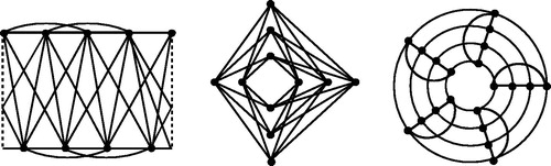
Fig. 1 Three graphs drawn in the plane so as to minimize the number of crossings. From left to right: K₈ drawn with 18 crossings, $K_{5,6}$ drawn with 24 crossings, and $C_5\times C_4$ drawn with 10 crossings. Note that in the drawing of K₈, the vertices in the top left and top right corners are identified.

It is a part of folklore that the complete graph K₅ and the complete bipartite graph $K_{3,3}$ cannot be drawn in the plane without any edges crossing. In 1930, it was proved by Kazimierz Kuratowski that these are essentially the only obstacles to graph planarity [8]. (This result was announced the same year by another pair of mathematicians, Orrin Frink and Paul Smith [4].)

Although the problem of joining with curves all pairs of a given set of points in the plane so that the number of crossings is minimized may have occurred to others, the first documented investigation was that of Anthony Hill, an English artist with no formal training in higher mathematics. In the 1950s, he found drawings that suggested a general formula for a bound on the crossing number of all complete graphs. (A precise definition of “crossing number” will be provided later.) The first graph in Figure 1 is a schematic adaptation of his drawings and shows K₈ with 18 crossings drawn on a tin can (equivalent to the plane). We will return to this shortly.

Somewhat surprisingly, complete graphs were not the first family of graphs to be studied for their crossing numbers. That honor goes to the family of complete bipartite graphs, and the problem of finding their crossing numbers arose from a wonderfully practical problem. Writing in the inaugural issue of The Journal of Graph Theory, Paul Turán describes how it came about [9]:

We worked near Budapest, in a brick factory. There were some kilns where the bricks were made and some open storage yards where the bricks were stored. All the kilns were connected by rail with all the storage yards. The bricks were carried on small wheeled trucks to the storage yards. …The trouble was only at the crossings. The trucks generally jumped the rails there, and the bricks fell out of them; in short, this caused a lot of trouble and loss of time …The idea occurred to me that this loss of time could have been minimized if the number of crossings of the rails had been minimized. But what is the minimum number of crossings? I realized after several days that the actual situation could have been improved, but the exact solution of the general problem with m kilns and n storage yards seemed to be very difficult.

An example of an optimal drawing of a complete bipartite graph is shown in the middle of Figure 1, which shows $K_{5,6}$ with 24 crossings. Further information regarding this history can be found in the essay by Robin Wilson and the present reviewer [1].

An example of a family of graphs that are embeddable on tori, but which have increasing crossing numbers, was provided in work by Harary, Kainen, and Schwenk. They showed that the products of cycles $C_r\times C_s$ have this property, and they conjectured that when $r\le s$ the minimum number of crossings is $r(s-2)$. The third graph in Figure 1 is an example of this for $C_5\times C_4$.

As it happens, the crossing number is not known for all of the graphs in any of the three families. The first two, the complete graphs and the complete bipartite graphs, are discussed in Chapter 1 of the present book, while the products of cycles are discussed in Chapter 2. One feature of these results is that they give the first “natural” families of graphs for which arbitrarily large crossing numbers are known precisely.

With that as background, we now turn to describing some of the interesting material in the individual chapters. Part of the appeal of this subject is that, as we shall see, there are some unexpected results.

Although the concept of crossing edges in a graph seems natural, it is important to be precise when counting the number of crossings. A drawing of a graph in the plane typically presents the vertices as points and the edges as arcs joining two vertices and containing none of the other vertices. It is assumed that edges are never tangent to one another and that at most two edges go through any point in the plane that is not a vertex. A drawing is said to be good if no edge crosses itself, if two adjacent edges never cross, and if nonadjacent edges cross at most once. The crossing number of a graph G, denoted cr(G), is defined as the minimum number of crossings of edges in any good drawing of G. Much of the first chapter is devoted to the two original families investigated by graph theorists.

A brief synopsis of the current status of affairs is the following:

• For complete graphs, the crossing number satisfies the bound$$\text{cr}\left(K_n\right)\le \frac{1}{4}\lfloor \frac{n}{2}\rfloor \lfloor \frac{n-1}{2}\rfloor \lfloor \frac{n-2}{2}\rfloor \lfloor \frac{n-3}{2}\rfloor .$$

  Equality is conjectured to hold in all cases, but is known to hold only for $n\le 12$. For n = 13, all that is known is that the crossing number is one of the four values 219, 221, 223, or 225.A construction that establishes the general upper bound is suggested by the first drawing in Figure 1. Informally, for n even, put half the vertices on each rim of a tin can. Then, with the minimum known numbers of crossings, join all of the vertices on each lid and join all pairs of vertices on different lids. For n odd, simply remove one vertex from the construction for the next even number.As it happens, there is also a nice drawing of K₉ with 36 crossings (the optimal number) in which each of the nine copies of K₈ has more than the optimal 18 crossings. This suggests that a proof of the conjecture using induction could be more complicated than might be expected.

• For complete bipartite graphs, the crossing number satisfies the bound$$\text{cr}\left(K_{r,s}\right)\le \lfloor \frac{r}{2}\rfloor \lfloor \frac{r-1}{2}\rfloor \lfloor \frac{s}{2}\rfloor \lfloor \frac{s-1}{2}\rfloor .$$

Again it is conjectured that equality holds in all cases. For $r\le s$, the only values of r for which equality is known to hold for all s are $r\le 6$. The exact value is known in a few other cases: for r = 7 or 8 and $s\le 10$. The upper bound is established by the simple construction illustrated by the second graph in our figure: Split r vertices into two sets as nearly equal as possible and place them on the positive and negative portions of the x-axis, then place the s vertices similarly on the y-axis, and finally join all pairs of vertices on different axes with line segments. The result achieves the given upper bound.

In his book, one of the first questions Schaefer raises concerns a variation in which the drawings need not be good. That is, adjacent edges are allowed to cross but these crossings are not counted. This is called the independent crossing number, and it clearly cannot exceed the crossing number itself. Interestingly, it is not known whether or not the two are always equal.

The third of our three original families is discussed in Chapter 2, and is a topic of personal interest to me. Following on the above-mentioned conjecture that$$\text{cr}(C_r\times C_s)=(r-2)s \text{for} r\le s,$$a colleague and I proved that it holds for r = 3 and 4, the first families of graphs other than the complete bipartite graphs for which arbitrarily large crossing numbers were determined. This result has since been extended up through r = 7. A further major result is that the formula also holds for all r and s if $s\ge r(r-1)$; hence, for all r, $\text{cr}(C_r\times C_s)$ is known except possibly for finitely many values of s.

Another interesting topic in this chapter is the problem of counting the number of uncrossed edges in a drawing of a graph. The chapter includes these results: For $n\ge 8$, there is a good drawing of K_n in which every edge is crossed, while at the other extreme, the greatest number of uncrossed edges in a good drawing of K_n is $2(n-1)$. With regard to the more general question of uncrossed subgraphs, it is proved that every good drawing of K_n has a crossing-free subgraph with minimum degree at least 2 and at least $3(n-1)/2$ edges.

Chapter 3 is devoted to other parameters related to the drawing of graphs. Two of these have a similar flavor: Given a graph G, the skewness, denoted by $\text{sk}(G)$, is the minimum number of edges in a set whose removal from G leaves a planar graph, and the edge crossing number, denoted by $\text{ecr}(G)$, is the minimum number of edges having crossings, taken over all good drawings of G. Some observations on these parameters are that $\text{sk}(G)\le \text{cr}(G)$ and $\text{ecr}(G)\le 2\text{cr}(G)$. It is also noted that there exist graphs with skewness 1 for which the crossing number is arbitrarily large; in other words, one edge has all of the crossings.

The most interesting connection between the crossing number and the other parameters is with the chromatic number. Bounds between the two were established that led Mike Albertson to make this conjecture: If $\chi (G)\ge k$, then $\text{cr}(G)\ge \text{cr}(K_k)$. This has been proved only for $k\le 16$.

The highlight of the next chapter, “Complexity and Algorithms,” is the classic result of Garey and Johnson: the crossing number problem is NP-complete [5]. It is interesting that the proof of the problem’s hardness uses a result that does not seem to be closely related to crossings, the “multiway cut problem”: Given an integer k and three vertices in a graph G, does G have a set of at most k edges whose removal leaves the three vertices in different components? It is also known that it can be decided in linear time whether or not, for a given positive integer k, it is true that $\text{cr}(G)\le k$. However to quote the author, “the proof is not suitable for implementation.”

The next two chapters address interesting natural concepts and are especially enjoyable since some of the results are surprising. They focus on drawings in the plane in which all of the edges are line segments. It was initially shown by Wagner in 1936 that every planar graph can be drawn in this way. As it happens, however, this result has come to be known as Fáry’s theorem even though Fáry did not publish it until 1948 [3]. (Fortunately, Wagner has his name attached to other results.) This concept leads to the concept of “rectilinear” drawings and the rectilinear crossing number, denoted by $\overline{\text{cr}}(G)$, defined as expected. Clearly, $\overline{\text{cr}}(G)\ge \text{cr}(G)$, and so a natural question is whether, given a graph G, equality holds or not.

Looking at this for complete graphs, we find that $\overline{\text{cr}}(K_n)=\text{cr}(K_n)$ when $n\le 7$, but the two are not equal when n = 8. However, rather unexpectedly, equality again holds for n = 9. One implication of this is that no optimal straight-line drawing of K₉ contains an optimal drawing of K₈. An even more surprising result is that, even though $\text{cr}(K_n)$ is known only through n = 12, $\overline{\text{cr}}(K_n)$ is known through n = 27 (and also for n = 30, for which the value is 9726). Because of the drawings used to get the upper bounds for the crossing numbers of our other two featured families, complete bipartite graphs and products of cycles clearly have rectilinear versions; it would be surprising if the two parameters were not equal in all cases.

Bienstock and Dean showed that Fáry’s theorem can be strengthened to include all graphs with crossing number 3 or less [2]. That is, if $\text{cr}(G)\le 3$, then $\overline{\text{cr}}(G)=\text{cr}(G)$, a result that is not too surprising. What is surprising is what happens next. Not only does the extension of Fáry’s theorem not hold, but there are graphs with ordinary crossing number 4 for which the rectilinear crossing number is arbitrarily large.

There are, of course, other concepts developed in these two chapters, but we now move on to Chapter 7, which is about another type of crossing number. The local crossing number $\text{lcr}(G)$ of G is the minimum, among all possible drawings of G in the plane, of the maximum number of crossings of any of the individual edges of the graph. In this definition, sloppiness was not the reason for omitting the adjective “good”: Another surprising result is that there are graphs for which a local crossing number of 4 is achieved in a drawing only if some adjacent edges are crossed.

Determining whether a graph has local crossing number 1 is already NP-complete, even though there is a linear algorithm for determining whether a graph is planar. For this reviewer, an even bigger surprise came in learning that the rectilinear local crossing number of all complete graphs has been found:$$\begin{array}{c}\overline{\text{lcr}}\left(K_n\right)=\lceil \frac{1}{2}\lceil \frac{n-3}{3}\rceil \lceil \frac{2(n-3)}{3}\rceil \rceil ,\text{except} \text{that}\\ \overline{\text{lcr}}\left(K_8\right)=4 \text{and} \overline{\text{lcr}}\left(K_{14}\right)=15.\end{array}$$

Chapters 8 through 11 involve other types of crossing numbers, but we mention them only briefly. Chapter 8 focuses on two types of drawings. First, the union of a number of half-planes with a common boundary line is called a book and the common boundary its spine. In the basic version, a drawing in a book has the vertices on the spine and each edge in just one of the half-planes. Second, in a monotone drawing, the plane has the Cartesian coordinate system, with all of the vertices on different vertical lines and no edge crossing any vertical line more than once.

The main subject of Chapter 9 again does not require drawings to be good. The pair crossing number, denoted by $\text{pcr}(G)$, is defined to be the minimum number of pairs of edges that cross in any drawing of graph G. Here we quote the author:

By definition pcr $\le$ cr, and it has been conjectured (and the author of this book is happy to follow suit), which would make irrelevant most of the results [here]. Intuitively, the conjecture seems plausible, as it seems difficult to imagine how multiple crossings between edges can be advantageous; however, attempts at proving equality, even for restricted models, via local redrawing very quickly runs into obstacles (flipping two crossing arcs can increase the pair crossing number of the drawing), and current global redrawing techniques seem to have reached a limit, ….

The inspiration for the material in Chapter 10 is the thickness of a graph, defined to be the minimum number of planar subgraphs in a set whose union is the given graph. If, instead of requiring each of the subgraphs to be planar, we fix the number of subgraphs to be, say, k, then the resulting parameter is the k-planar crossing number. The variation considered in Chapter 11 counts in a drawing only the number of pairs of edges that cross an odd number of times. Intuitively, it would seem that this number should be just the crossing number itself, but, in another counter-intuitive result, this is not always the case.

The book concludes with a chapter on maximizing the number of crossings in good drawings of graphs. One of the oldest problems of this type goes back to 1885, when Richard Baltzer asked for the largest number of crossings there can be in an n-sided polygon. (The answer is $n(n-3)/2$ if n is odd and $n(n-4)/2+1$ if n is even.) If we consider this as a graph problem, then we are looking at rectilinear drawings, but the corresponding general question is also interesting and was answered by Harborth [7]. The answer is now the same for any number of sides (except for n = 4) as it was before only for an odd number: the maximum crossing number of the cycle C_n is $n(n-3)/2$ for $n\ge 5$. Harborth also solved the problem for the two basic families that opened the book: The maximum crossing number of the complete graph K_n is $\left(\begin{array}{c}n\\ 4\end{array}\right)$ and that of the complete bipartite graph $K_{r,s}$ is $\left(\begin{array}{c}r\\ 2\end{array}\right)\left(\begin{array}{c}s\\ 2\end{array}\right)$. In both cases, the values can be achieved by rectilinear drawings.

A thrackle is defined to be a graph having a drawing in which every pair of nonadjacent edges cross. We conclude our description of the book’s highlights with a long-standing conjecture by John Conway: No thrackle has more edges than vertices.

As the reader should have gathered, it is the reviewer’s opinion that this book is a valuable contribution to mathematics. In addition to the multitude of results presented (most of which are proved), there are a couple of other features worth mentioning. These include interesting notes and exercises at the end of each chapter as well as useful appendices on the basics of topological graph theory and complexity theory.

In the spirit of exposition for which the MAA is noted, I think that there are a few improvements that could have been made (and that might be considered for a second edition). Although there do not seem to be many typographical errors, there were a few that were easily spotted, including this one: On page 73, in the discussion of Albertson’s work, there is “Alberston, …the truth of Albertston’s conjecture.” One peeve I have is the use of personal pronouns in the statements of theorems. For example, in Theorem 1.32 on page 29, there is “If we place n vertices …”—the truth of the result doesn’t depend on anyone placing vertices, does it? In the interest of elegance, I like having theorems numbered consecutively. For instance, why should the first theorem be numbered 1.8? (Even if lemmas are included in the sequence, why is a Remark (page 6)?)

Returning to the positive aspects of the book, I want to express my thanks to the author for writing the book and to add my thanks to his where he wrote in the Acknowledgments: “This book was written at the invitation of Miklos Bona, and I would like to give belated thanks to Dan Archdeacon for suggesting my my name to him in the first place; [and to others].”

Edited by Darren Glass
Department of Mathematics, Gettysburg College, Gettysburg, PA 17325
Reviewed by Lowell Beineke
Purdue University, Fort Wayne, Indiana 46805
[email protected]

References

- Beineke, L., Wilson, R. (2010). The early history of the brick factory problem. Math. Intell. 32(2): 41–48. DOI: 10.1007/s00283-009-9120-4.
- Bienstock, D., Dean, N. (1993). Bounds for rectilinear crossing numbers. J. Graph Theory. 17(3): 333–348. DOI: 10.1002/jgt.3190170308.
- Fáry, I. (1948). On straight line representation of planar graphs. Acta Univ. Szeged. Sect. Sci. Math. 11: 229–233.
- Frink, O., Smith, P. A. (1930). Irreducible non-planar graphs. Bull. AMS. 36(3): 214. doi.org/10.1090/S0002-9904-1930-04929-0.
- Garey, M. R., Johnson, D. S. (1983). Crossing number is NP-complete. SIAM J. Alg. Disc. Methods. 4(3): 312–316. DOI: 10.1137/0604033.
- Harary, F., Kainen, P. C., Schwenk, A. J. (1973). Toroidal graphs with arbitrarily high crossing numbers. Nanta Math. 6(1): 58–67.
- Harborth, H. (1976). Parity of numbers of crossings for complete n-partite graphs. Math. Slovaca. 2(2): 77–95. DOI: 10.1016/S0012-365X(01)00078-4.
- Kuratowski, K. (1930). Sur le probème des courbes gauches en topologie. Fund. Math. 15(1): 271–283. DOI: 10.4064/fm-15-1-271-283.
- Turán, P. (1977). A note of welcome. J. Graph Theory. 1(1): 7–9. DOI: 10.1002/jgt.3190010105.