l’Hôpital’s Rule for Multivariable Functions

Abstract

Zero divided by zero is arguably the single most important concept underlying calculus. For functions of more than one variable, methods of proof for indeterminate limits are not as familiar as for functions of a single variable. We present a l’Hôpital’s rule that provides a way to simplify and resolve a wide variety of zero-over-zero limits in terms of quotients of their derivatives.

• MSC: Primary 26B12

1 Introduction

It is interesting to reflect on how many times in mathematics the word “impossible” only means “you’re not ready to understand that yet.” At different stages of school we may be instructed that it is impossible to subtract 3 minus 5, or to take the square root of 6, or to take the square root of –1, only to find later that these were only impossible within the given framework that we knew. And even in mathematical research, a generally agreed-upon impossibility may melt away in the presence of a context-expanding new insight.

Now what about zero divided by zero? We are sternly informed in school that dividing by zero is impossible and must be shunned. Does that prohibition ever get softened?

In fact, a more accurate statement, (once we are ready to understand it) is that it is impossible to divide zero by zero out of context. All other arithmetic operations are independent of context, a rather remarkable fact. So six divided by three equals two, no matter whether you are sharing expenses with a couple of friends or making a fraction of a recipe of bread. Not so with zero divided by zero: if you take a photograph of two racecars and observe that in the picture both cars travel zero feet in zero seconds, that is no help in comparing the cars’ velocities.

But if you can find some contextual information to a zero-over-zero problem, like a sequence or a quotient of functions, then you are back in business.

In 1696 the Marquis de l’Hôpital published the first calculus text, in which was revealed the elegant and enduring rule that bears his name. Single-variable indeterminate limits were thus supplied with a go-to method of resolution.

However, methods for resolving indeterminate limits in several variables are not as universally established. A calculus textbook will usually tell how to prove certain multivariable limits do not exist, by restricting the domain to individual lines through the singular point and obtaining different limits. This is followed by a warning not to try a proof using the same method to claim that a limit does exist. A standard counterexample is $x^{2}y/(x^4+y^2)$ as $(x,y)\to (0,0)$, whose limit along each line through the origin is zero, but along the parabola $y=x^2$ its limit is 1/2.

The student may then naturally ask what is the right way to prove existence of a multivariable limit, but may find this question addressed only partially. What about a l’Hôpital’s rule for multivariable functions? At one point the present author knew why such a rule was impossible; we will comment further on this below, where we will also acknowledge the vital contribution of an anonymous referee.

Papers by Dobrescu and Siclovan [3] and Young [9, p. 71], both present a very specific version of l’Hôpital’s rule for a two-variable indeterminate limit resolvable by taking the mixed second derivative ${\partial }^2/\partial x\partial y$ of the numerator and denominator functions.

A paper of Fine and Kass [4] has a version using first-order derivatives, taking directional derivatives always in the direction toward the singular point. While this version provides an interesting perspective, it seems difficult to find examples where the rule simplifies the functions and resolves the limit.

Carter [2] discusses when l’Hôpital’s rule does and does not work for complex-valued functions.

Kishka et al. [5] prove that l’Hôpital’s rule works for matrix functions under certain circumstances; an example they give is that the limit of $\text{sin}\hspace{0.17em}(X)X^{-1}$, as the n-by-n matrix X approaches the zero matrix, is the identity matrix.

There are some papers with a good treatment of the indeterminate limit of a quotient of a vector-valued function over a real-valued function, but these papers concern functions of a single variable. See the Rosenholtz paper [7], as well as papers by Albrycht [1], Popa [6], and Wa$\stackrel{.}{\mathrm{z}}$ewski [8] for l’Hôpital-style theorems of this type.

2 Features and difficulties

The expanded territory in the multivariable setting is both a feature and a challenge. On the one hand, it provides for a novel type of singularity not possible with single-variable functions. On the other hand, the potential difficulties will require side hypotheses as well as the extra step of working out which partial (and iterated partial) derivatives to include in the comparison.

Unlike the single-variable setting, a zero-over-zero singularity can be nonisolated, as with the function(1) $$\frac{f(x,y)}{g(x,y)}=\frac{x-y}{\hspace{0.17em}\text{sin}\hspace{0.17em}x-\hspace{0.17em}\text{sin}\hspace{0.17em}y}.$$(1)

In such a case, when we take the limit we implicitly exclude the points where g = 0 from the domain.

This function has a limit of 1 as we approach the origin, as Theorem 4 will prove. The limit is suggested by the quotients$$\frac{f_x(0,0)}{g_x(0,0)}=\frac{f_y(0,0)}{g_y(0,0)}=1.$$

But we need to take more care than just examining the derivatives, as shown by the function(2) $$\frac{f(x,y)}{g(x,y)}=\frac{x-\hspace{0.17em}\text{sin}\hspace{0.17em}y}{\hspace{0.17em}\text{sin}\hspace{0.17em}x-y},$$(2) whose graph is shown in Figure 1(a). Near zero, the numerators of (1) and (2) are very nearly the same, as are their denominators. The first partial derivatives might suggest that the limit of (2) is also 1, but this is not the case. In the second example, the set of points where $f(x,y)=0$ does not contain the set where $g(x,y)=0$, so we can find points arbitrarily near the origin at which g is much closer to 0 than is f; thus, the quotient f/g is unbounded as we approach the origin.

Fig. 1 Graphs of examples discussed above.

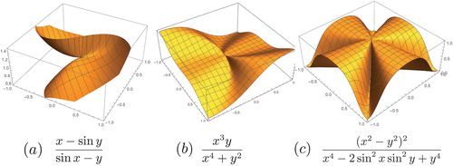
This type of counterexample originally caused the author to believe that a l’Hôpital’s rule could not exist for multivariable functions. Not until later did the resolution of this problem present itself; we simply make the side hypothesis that the zero set of f contain that of g within a neighborhood of the singularity.

The author was also perplexed by examples with isolated singularities such as(3) $$\frac{x^{k}y}{x^4+y^2};$$(3) see Figure 1(b) for the graph when k = 3. When k > 2, the limit at the origin is zero, and when $k\le 2$, the limit does not exist, as shown by approaching the origin along the curves $y=m{x}^2$ for different values of m. But which quotient(s) of partial derivatives would establish this result?

The author’s disbelief in the existence of a l’Hôpital’s rule for isolated singularities persisted for years after finding a result for the nonisolated case. Indeed, the first submission of the present article did not include a rule for isolated singularities. The author is most grateful for an anonymous referee’s reassuring disbelief in the nonexistence of that vital part of l’Hôpital’s rule, and his or her suggestion to look at different pathways toward the singular point. (Not lost on the author is the historical precedent for anonymity in contributing to l’Hôpital’s rules!)

The key turns out to be understanding which groups of iterated partial derivatives to divide and compare, and then finding the right curves along which to approach the singular point; see Theorem 5.

As with the nonisolated singularities, we must check one side hypothesis, as illustrated by the example$$\underset{(x,y)\to (0,0)}{\lim }\frac{{(x^2-y^2)}^2}{x^4-2{\hspace{0.17em}\text{sin}\hspace{0.17em}}^{2}x{\hspace{0.17em}\text{sin}\hspace{0.17em}}^{2}y+y^4};$$see Figure 1(c). This limit does not exist, as shown by examining the function restricted (in turn) to each of the lines y = x and $y=2x$. The derivative quotients prescribed in our l’Hôpital’s rule below do not detect the subtlety inherent in this example. We resolve this by requiring as a side hypothesis that a Taylor polynomial of the denominator have an isolated zero at (0, 0).

3 l’Hôpital’s rule

Our l’Hôpital’s rule will have three parts, grouped into the two theorems of the present section, together covering a considerable range of zero-over-zero, indeterminate limits. The strategy of proof in all cases will be to apply the generalized mean value theorem to restrictions of the multivariate functions along certain paths, namely straight lines, paths of steepest ascent or descent of the denominator function $g(\mathit{x})$, and paths parameterized using certain integer powers of t.

Note that the standard single-variable l’Hôpital’s rule includes cases that allow infinity to play various roles in the limits. In the present article, we omit infinite limits, leaving them for future research.

We begin by proving a result giving some basic control over the behavior of paths of steepest change, ensuring that they cannot wander too far.

Lemma 1.

Let h be a $C^{1,1}$ function on an open set $\mathcal{N}$ with $h(\mathit{p})=0$ for some $\mathit{p}\in \mathcal{N}$ and $\nabla h\ne 0$ in $\mathcal{N}$ except possibly at p. Then for any $ϵ>0$ there exists $\delta \in (0,ϵ)$ such that for every ${\mathit{x}}_0\in B_{\delta }(\mathit{p})$ at which $h({\mathit{x}}_0)$ is positive (respectively, negative), a path of steepest descent (respectively, ascent) of h from ${\mathit{x}}_0$ cannot leave $B_{ϵ}(\mathit{p})$ before reaching the value $h(\mathit{x})=0$.

Proof.

We may restrict attention to $ϵ$ sufficiently small so that the closure of the ball $B_{ϵ}(\mathit{p})$ is contained in $\mathcal{N}$. Given such an $ϵ$, let k > 0 be the minimum value of $\left|\right|\nabla h\left|\right|$ in the annulus $A:ϵ/2\le \left|\right|\mathit{x}-\mathit{p}\left|\right|\le ϵ$. Then given any path of steepest ascent or descent of h beginning at a point closer to p than distance $ϵ/2$, if the path could extend further from p than distance $ϵ$, then $h(\mathit{x})$ must change by at least $kϵ/2$ as the path passes through A. Thus, we need only choose $\delta >0$ sufficiently small so that within $B_{\delta }(\mathit{p}),|h(\mathit{x})|<kϵ/2$, and the result will follow.■

Definition 2.

Let $k_i\in \mathbb{N}$ for each i. Let $S=S(k_1,\dots ,k_n)$ be the $(n-1)$-simplex in ${\mathbb{R}}^n$ with vertices on the axes at $\left\{k_i{\mathbf{e}}_i\right\}$. For any nonnegative integer lattice point $\mathit{q}=(q_1,\dots ,q_n)$, let $D_{\mathit{q}}$ be the differential operator that differentiates a function q_i times by each variable x_i .

For any $\alpha \in {\mathbb{Z}}^n$ with nonnegative integer entries we say α lies below $S(k_1,\dots ,k_n)$ if α is not in S but lies on the same side of S as the origin. Let the simplicial Taylor polynomial $T_{\mathrm{}{\mathrm{}}_S}g(\mathit{x})$, centered at p, be the polynomial satisfying $D_{\alpha }T(\mathit{p})=0$ for all $\alpha \notin S$ and $D_{\alpha }T(\mathit{p})=D_{\alpha }g(\mathit{p})$ for all $\alpha \in S$.

We say a $C^{\infty }$ function g is dominant at p with respect to $S(k_1,\dots ,k_n)$ if

1. the pure partial derivatives $D_{k_i{\mathbf{e}}_i}g(\mathit{p})$ are all nonzero,

2. the pure and mixed partial derivatives $D_{\alpha }g(\mathit{p})$ are zero for all lattice points α below S, and

3. the simplicial Taylor polynomial $T_{{\mathrm{}}_S}g(\mathit{x})$ has an isolated zero at p, which will require in particular that each k_i is an even integer.

We will use the $D_{\alpha }$ notation in connection with Theorem 5 and its supporting Lemma 3. Elsewhere a simple subscript notation for partial derivatives will be more convenient.

Lemma 3.

Let $\mathcal{N}$ be an open neighborhood of $\mathit{p}=(p_1,\dots ,p_n)\in {\mathbb{R}}^n$ and let $g:\mathcal{N}\to \mathbb{R}$ be a $C^{\infty }$ function. Let $\mathbf{k}=(k_1,\dots ,k_n)$ with $k_i\in \mathbb{N}$ for each $i\in \{1,\dots ,n\}$, and let $x_i(t)=p_i+m_i{t}^{k_i}$ for each i, where each m_i is a free variable. Define $$G(t)=g(x_1(t),\dots ,x_n(t)).$$

Then for any $j\in \mathbb{N}$, the derivative satisfies $$G^{(j)}(0)=j!{\sum }_{\begin{array}{c}\mathit{q}·\mathbf{k}=j\\ q_i\in \mathbb{N}\cup \left\{0\right\}\end{array}}{D}_{\mathit{q}}g(\mathit{p})\prod \frac{m_i^{q_i}}{q_i!},$$which equals $j!$ times the sum of terms of the Taylor polynomial of g corresponding to the vectors $\mathit{q}$ that appear in the above sum, with each x_i replaced by m_i.

Proof.

We may assume that g is an analytic function, since the result only depends on the rules of differentiation, which will give the same results as long as g is sufficiently many times differentiable. For simpler notation assume p is the origin; otherwise we would subtract p_i from each x_i in what follows.

Let $c x_1^{q_1}\cdots x_n^{q_n}$ be a term of the power series for g. This term will only contribute to the jth derivative of $g(\mathit{x}(t))$ at t = 0 if $q_1{k}_1+\cdots +q_n{k}_n=j$. Plugging in the values $x_i(t)=m_i{t}^{k_i}$, the term becomes$$c m_1^{q_1}\cdots m_n^{q_n}{t}^j,$$whose jth derivative at t = 0 is(4) $$j! c m_1^{q_1}\cdots m_n^{q_n}.$$(4)

On the other hand, if we differentiate $g(\mathit{x})$ by each x_i q_i times, we get(5) $$c q_1!\cdots q_n!.$$(5)

Dividing (4) by (5) we obtain the desired expression.■

We are now ready to disprove the nonexistence of a l’Hôpital’s rule for multivariable functions.

Theorem 4

(l’Hôpital’s rule for multivariable functions, nonisolated singularities). Let f and g be $C^{\infty }$ functions defined in a neighborhood $\mathcal{N}$ of $\mathit{p}\in {\mathbb{R}}^n$. Suppose that within $\mathcal{N}$, whenever $g(\mathit{x})=0$ then $f(\mathit{x})=0$ as well. Then

1. If any first partial derivative $g_{x_i}(\mathit{p})$ is nonzero, then

   1. $\underset{\mathit{x}\to \mathit{p}}{\lim }\frac{f(\mathit{x})}{g(\mathit{x})}=\frac{f_{x_i}(\mathit{p})}{g_{x_i}(\mathit{p})}.$

2. If $\nabla g(\mathit{x})=0$ only at $\mathit{x}=\mathit{p}$, then $$\underset{\mathit{x}\to \mathit{p}}{\lim }\frac{f(\mathit{x})}{g(\mathit{x})}=\underset{\mathit{x}\to \mathit{p}}{\lim }\frac{f_{x_i}(\mathit{x})}{g_{x_i}(\mathit{x})}$$if the right-hand side exists (and is a finite real number, not infinity) and is equal for all i; this last limit is taken over x such that $$g_{x_i}(\mathit{x})\ne 0$$

Proof.

First consider claim 1. Since the partial derivative $g_{x_i}(\mathit{p})$ is nonzero, we can restrict to a possibly smaller neighborhood of p in which the derivative is everywhere nonzero.

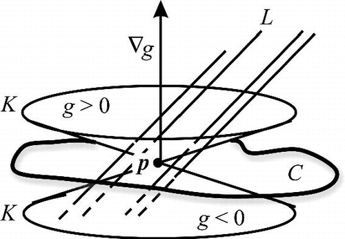
Let L be the line through p parallel to the x_i -axis, and let C be the level set g = 0. Again since $g_{x_i}(\mathit{p})$ is nonzero, L is transverse to C at p.

We need to know that lines parallel to L and sufficiently near L also cross C near p. Choose an angle θ strictly closer to $\pi /2$ than the angle between L and the normal $\nabla g$ to C. Form a double cone K as the union of lines through p that make an angle of θ with $\nabla g$; see Figure 2. Now the directional derivatives of g at p in the cone directions are all a positive constant for half the cone and its negative for the other half. Since g is $C^{1,1}$, in a small neighborhood B₂ of p these directional derivatives have constant sign. There is a smaller neighborhood B₃ of p such that all lines parallel to L that pass through B₃ must pass through both halves of K within B₂. These will therefore pass through points where g > 0 and points where g < 0; by the intermediate value theorem all such lines also pass, near p, through the zero set of g.

Fig. 2 Parallel lines crossing the zero set of g.

Now consider, as in Figure 3, any sequence $({\mathit{x}}_j)$ of points in B₃ converging to p, with $g({\mathit{x}}_j)\ne 0$ for all j. Let ${\mathit{z}}_j$ be the points guaranteed above, at which $g({\mathit{z}}_j)=0$ and ${\mathit{z}}_j-{\mathit{x}}_j$ is a scalar multiple of the coordinate vector e_i for each j. The points ${\mathit{z}}_j$ also converge to p.

Fig. 3 Sequences of points approaching a singularity.

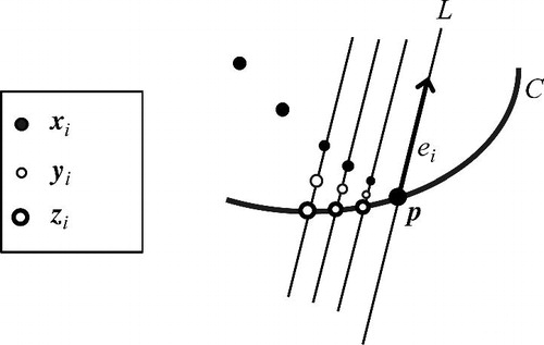
Now for each j, as in the proof of the single-variable l’Hôpital’s rule, apply the generalized mean value theorem to the quotient f/g restricted to the line L. We find that there is a point ${\mathit{y}}_j$, lying in between ${\mathit{x}}_j$ and ${\mathit{z}}_j$, such that$$\frac{f_{x_i}({\mathit{y}}_j)}{g_{x_i}({\mathit{y}}_j)}=\frac{f({\mathit{x}}_j)-f({\mathit{z}}_j)}{g({\mathit{x}}_j)-g({\mathit{z}}_j)}=\frac{f({\mathit{x}}_j)}{g({\mathit{x}}_j)}.$$

But now since the points ${\mathit{y}}_j$ also converge to p, the desired result follows.

Now consider claim 2 in the theorem. We will apply the generalized mean value theorem to f/g restricted to paths of quickest ascent or descent of g.

Let $\lambda \in \mathbb{R}$ be the common value of the limits of $f_{x_i}(\mathit{x})/g_{x_i}(\mathit{x})$.

Given ${ϵ}_1>0$, choose ${ϵ}_2>0$ such that for all $\mathit{x}\in B_{{ϵ}_2}(\mathit{p}),|f(\mathit{x})|<{ϵ}_1$ and such that for all i satisfying $g_{x_i}(\mathit{x})\ne 0$,$$|f_{x_i}(\mathit{x})/g_{x_i}(\mathit{x})-\lambda |<\frac{{ϵ}_1}{2}$$

so that(6) $$|f_{x_i}(\mathit{x})-\lambda g_{x_i}(\mathit{x})|<\frac{{ϵ}_1}{2}|g_{x_i}(\mathit{x})|.$$(6)

By Lemma 1 choose $\delta >0$ so that paths of steepest change of g beginning in $B=B_{\delta }(\mathit{p})$ remain within $B_{{ϵ}_2}(\mathit{p})$ up until g = 0.

Take a point ${\mathit{x}}_0\in B$ with $g({\mathit{x}}_0)\ne 0$. Without loss of generality, $g({\mathit{x}}_0)>0$.

Let $\mathit{x}(t),t\ge 0$, be a parameterization of a path of fastest decrease of g from ${\mathit{x}}_0$. A priori it might happen that $\mathit{x}(t)$ has infinite length without $g(\mathit{x}(t))$ ever reaching zero. But we do know at least that g nears zero in finite time. For if $g(\mathit{x}(t))$ were to stay above some $ϵ>0$, then $\mathit{x}(t)$ would have to stay outside some ball about the origin. But then by compactness and the fact that $\nabla g\ne 0,\left|\right|\nabla g\left|\right|$ would be bounded below by a positive quantity. This would force $g(\mathit{x}(t))$ to decrease to zero, a contradiction.

So $g(\mathit{x}(t))$ goes as near to zero as we wish in finite time. Now if $f(\mathit{x}(t))$ did not also converge to zero, there would exist ${ϵ}_3>0$ and a sequence $(t_i)$ with $g(\mathit{x}(t_i))\to 0$ but $|f(\mathit{x}(t_i))|>{ϵ}_3$ for all i. Then by compactness, a subsequence of $\mathit{x}(t_i)$ would converge to some ${\mathit{y}}_0$, forcing $g({\mathit{y}}_0)=0$ but $f({\mathit{y}}_0)\ne 0$, a contradiction.

Now $\mathit{x}\prime (t)$ is a scalar multiple of $-\nabla g(\mathit{x}(t))$ for each $t\in (0,t_0)$. By the chain rule and the generalized mean value theorem, there exists $c\in (0,t_0)$ such that$$\frac{f({\mathit{x}}_0)-f(\mathit{x}(t_0))}{g({\mathit{x}}_0)-g(\mathit{x}(t_0))}=\frac{\nabla f(\mathit{x}(c))·\mathit{x}\prime (c)}{\nabla g(\mathit{x}(c))·\mathit{x}\prime (c)}=\frac{\nabla f(\mathit{x}(c))·\nabla g(\mathit{x}(c))}{\nabla g(\mathit{x}(c))·\nabla g(\mathit{x}(c))}.$$

But since $f(\mathit{x}(t_0))$ and $g(\mathit{x}(t_0))$ can be made arbitrarily small, we can ensure that the quantity$$\left|\frac{f({\mathit{x}}_0)-f(\mathit{x}(t_0))}{g({\mathit{x}}_0)-g(\mathit{x}(t_0))}-\frac{f({\mathit{x}}_0)}{g({\mathit{x}}_0)}\right|$$is less than $\frac{1}{2}{ϵ}_1$. Then$$\left|\frac{f({\mathit{x}}_0)}{g({\mathit{x}}_0)}-\lambda \right|<\frac{1}{2}{ϵ}_1+\left|\frac{(\nabla f(\mathit{x}(c))-\lambda \nabla g(\mathit{x}(c)))·\nabla g(\mathit{x}(c))}{\nabla g(\mathit{x}(c))·\nabla g(\mathit{x}(c))}\right|.$$

Since the path x must stay within $B_{{ϵ}_2}(\mathit{p})$, by (6), the above expression is less than ${ϵ}_1$, as required.■

Theorem 5

(l’Hôpital’s rule for multivariable functions, isolated singularities).

Let f and g be $C^{\infty }$ functions in a neighborhood $\mathcal{N}\subseteq {\mathbb{R}}^n$, with f and g equaling zero only at p. For each i let ${\mathcal{l}}_i$ be the smallest natural number such that the pure iterated partial $D_{{\mathcal{l}}_i{\mathbf{e}}_i}g(\mathit{p})$ is nonzero. Let S be the simplex whose vertices are the points $\left\{{\mathcal{l}}_i{\mathbf{e}}_i\right\}$. If g is dominant (Definition 2) then the limit of f/g exists and equals $\lambda \in \mathbb{R}$, if $D_{\alpha }f(\mathit{p})=\lambda D_{\alpha }g(\mathit{p})$ for all α lying in or below S.

Conversely, if $D_{\alpha }g=0$ for all α below S but there does not exist such a λ, then the limit of f/g does not exist.

Proof. A

s before, for simplicity’s sake assume that the singularity p is at the origin. Work within a closed ball $C=B_r(0)$ inside $\mathcal{N}$ within which $T_{{\mathrm{}}_S}g$ is zero only at 0.

Assume first that such a λ does exist. We note that$$\frac{f(\mathit{x})}{g(\mathit{x})}=\frac{f(\mathit{x})}{T_{{\mathrm{}}_S}g(\mathit{x})}÷\frac{g(\mathit{x})}{T_{{\mathrm{}}_S}g(\mathit{x})}.$$

Thus it will suffice to prove the theorem with a simplicial polynomial as the denominator; then λ will equal 1 when we apply the theorem to $g/(T_{{\mathrm{}}_S}g)$, and we can divide the limits of $f/(T_{{\mathrm{}}_S}g)$ and $g/(T_{{\mathrm{}}_S}g)$ to obtain the desired result. (The advantage is to make it easier to verify the hypothesis that the denominator have nonzero derivative when applying the Cauchy mean value theorem.)

Let L be the least common multiple of $({\mathcal{l}}_1,\dots ,{\mathcal{l}}_n)$, and set $k_i=L/{\mathcal{l}}_i$ for each i. The key idea is to approach the origin along curves(7) $${\gamma }_{\mathbf{x}}(t)=(x_1{t}^{k_1},\dots ,x_n{t}^{k_n})$$(7) for $\mathbf{x}\in \partial B_r(0)$ and $t\in (0,1]$.

Given any starting point $\mathit{z}\ne 0$ in $B_r(0)$, by continuity we can choose $t_0\ge 1$ such that$$\left|\right|(z_1{t}_0^{k_1},\dots ,z_n{t}_0^{k_n})\left|\right|=r.$$

Let $x_i=z_i{t}_0^{k_i}$; then $\mathbf{x}\in B_r(0)$, and the path (7) lies in $B_r(0)$ and passes through z when $t=1/t_0$.

Define$$F(t)=F_{\mathit{x}}(t)=f({\gamma }_{\mathit{x}}(t)) \mathrm{ }\text{and}\mathrm{ } G(t)=G_{\mathit{x}}(t)=T_{{\mathrm{}}_S}g({\gamma }_{\mathit{x}}(t)).$$

Apply the Cauchy mean value theorem to $F_{\mathit{x}}(t)/G_{\mathit{x}}(t)$ on the interval $t\in [0,1/t_0]$. We obtain$$\frac{f(\mathit{z})}{g(\mathit{z})}=\frac{F_{\mathit{x}}(1/t_0)}{G_{\mathit{x}}(1/t_0)}=\frac{F{\prime }_{\mathit{x}}(c_1)}{G{\prime }_{\mathit{x}}(c_1)}$$

for some $c_1\in (0,1/t_0)$. Repeat the application L – 1 more times, obtaining in the end that$$\frac{f(\mathit{z})}{g(\mathit{z})}=\frac{\frac{d^L}{d{t}^L}{F}_{\mathit{x}}(c_L)}{\frac{d^L}{d{t}^L}{G}_{\mathit{x}}(c_L)}=\frac{\frac{d^L}{d{t}^L}{F}_{\mathit{x}}(c_L)}{\frac{d^L}{d{t}^L}{G}_{\mathit{x}}(0)}$$for some $c_L\in (0,1/t_0)$; the last equation follows because $G_{\mathit{x}}$ is a simplicial polynomial and the denominator is a function only of x and is constant in t.

By Lemma 3, for fixed x the limit as $t\to 0$ of $F_{\mathit{x}}(t)/G_{\mathit{x}}(t)$ equals λ; we need only be concerned about the uniformity of that limit.

Let W be the (positive) minimum value of the coefficient of t^L in $G_{\mathit{x}}(t)$, for x satisfying $\left|\right|\mathit{x}\left|\right| = r$. Then$$\begin{array}{c}\frac{F_{\mathit{x}}^{(L)}(c_L)}{G_{\mathit{x}}^{(L)}(0)}-\lambda =\frac{F_{\mathit{x}}^{(L)}(c_L)-F_{\mathit{x}}^{(L)}(0)}{G_{\mathit{x}}^{(L)}(0)}\\ \le \frac{F_{\mathit{x}}^{(L)}(c_L)-F_{\mathit{x}}^{(L)}(0)}{L! W}.\end{array}$$

Now by the (regular) mean value theorem, the numerator equals c_L times the $(L+1)$st derivative of F evaluated at some $t\in (0,c_L)$. So there is a constant X depending on finitely many derivatives of f, which in turn are bounded on $B_r(0)$, such that$$\frac{f(\mathit{z})}{g(\mathit{z})}-\lambda <\frac{X{c}_L}{L! W}<\frac{X}{t_{0}L! W}.$$

Since $t_0\to \infty$ as $\mathit{z}\to 0$, the limit of this discrepancy is zero.■

4 Examples

We now give five examples whose analysis is straightforward given l’Hôpital’s rule, leaving the reader to resolve them. The sixth example is a bit fancier.

1. $\underset{(x,y)\to (0,0)}{\lim }\frac{2{\hspace{0.17em}\text{tan}\hspace{0.17em}}^{2}x+y^2}{x^2+1-\hspace{0.17em}\text{cos}\hspace{0.17em}y}$

2. $\underset{(x,y,z)\to (0,0,0)}{\lim }\frac{\hspace{0.17em}\text{sin}\hspace{0.17em}z-\hspace{0.17em}\text{sin}\hspace{0.17em}(x^2+y^2)}{\hspace{0.17em}\text{tan}\hspace{0.17em}(z-x^2)-\hspace{0.17em}\text{tan}\hspace{0.17em}(y^2)}$

3. $\underset{(x,y)\to (0,0)}{\lim }\frac{x^2-y^2}{\hspace{0.17em}\text{cos}\hspace{0.17em}x-\hspace{0.17em}\text{cos}\hspace{0.17em}y}$

4. $\underset{(x,y)\to (0,0)}{\lim } \frac{\hspace{0.17em}\text{cos}\hspace{0.17em}x+x{y}^3-{\hspace{0.17em}\text{sin}\hspace{0.17em}}^{4}y-1}{{\hspace{0.17em}\text{sin}\hspace{0.17em}}^{2}x+2y^4}$

5. $\underset{(x,y)\to (0,0)}{\lim }\frac{x^{\alpha }y}{x^4+y\hspace{0.17em}\text{sin}\hspace{0.17em}y}$ for each $\alpha \ge 0$

6. $\underset{(x,y)\to (0,0)}{\lim }\frac{x^{5}y}{x^6+x^2{y}^2+y^6}$.

Hint: The hypotheses of l’Hôpital’s rule are not satisfied in the last example because the points (6, 0), (2, 2), and (0, 6) are not collinear, but try imbedding the problem into three dimensions by setting z = xy and eliminating some of the occurrences of y.

Acknowledgments

The author is most grateful to the second referee for suggesting the existence of the rule for isolated singularities, and sketching an idea of how it might be done.

Additional information

Notes on contributors

Gary R. Lawlor

GARY LAWLOR is an associate professor at his alma mater, Brigham Young University, with a Ph.D. from Stanford. Previously he was an instructor and assistant professor at Princeton from 1988 to 1991. One of the principal moving forces in his research has been the insatiable hunger to know: Is there a simpler way?

He is a husband, dad, grandpa and BYU sports fan, and an avid genealogist and student of ancient and modern scripture, but has no idea how to apply l’Hôpital’s rule to any of these pursuits.

References

- Albrycht, J. (1951). L’Hôpital’s rule for vector-valued functions. Colloq. Math. 2: 176–177. DOI: 10.4064/cm-2-3-4-176-177.
- Carter, D. S. (1958). L’Hospital’s rule for complex-valued functions. Amer. Math. Monthly. 65(4): 264–266. DOI: 10.2307/2310244.
- Dobrescu, E., Siclovan, I. (1965). Considerations on functions of two variables. Analele Universitatii Timisoara Seria Stiinte Matematica-Fizica. 3: 109–121.
- Fine, A. I., Kass, S. (1966). Indeterminate forms for multi-place functions. Ann. Polon. Math. 18: 59–64. DOI: 10.4064/ap-18-1-59-64.
- Kishka, Z. M., Abul-Ez, M., Saleem, M., Abd-Elmageed, H. (2013). L’Hospital rule for matrix functions. J. Egyptian Math. Soc. 21(2): 115–118. DOI: 10.1016/j.joems.2013.01.007.
- Popa, D. (1999). On the vector form of the Lagrange formula, the Darboux property and l’Hôpital’s rule (English summary). Real Anal. Exchange. 25(2): 787–793. DOI: 10.2307/44154034.
- Rosenholtz, I. (1991). A topological mean value theorem for the plane. Amer. Math. Monthly. 98(2): 149–154. DOI: 10.2307/2323948.
- Wazewski, T. (1951). Une généralisation des théorèmes sur les accroissements finis au cas des espaces de Banach et application a la généralisation du théorème de l’Hôpital. Ann. Soc. Polon. Math. 24(2): 132–147.
- Young, W. H. (1910). On indeterminate forms. Proc. Lond. Math. Soc. 2(8): 40–76. DOI: 10.1112/plms/s2-8.1.40.