Complex Methods for Bounds on the Number of Periodic Solutions with an Application to a Neural Model

Abstract

The qualitative behavior of the differential equation $x\prime =f(t,x)$, where x is real and f is periodic in t, is determined by the attracting periodic solutions. This article gives an exposition of a method of Ilyashenko that uses complex analysis to determine an upper bound on the number of periodic solutions. The method is then applied to a well-known model of a single neuron or pool of neurons.

MSC::

• Primary 34C25
• Secondary 30E99
• 92C20

1 Introduction

The value of many real-valued quantities at time t can often be modeled by a differential equation of the form $x\prime =f(t,x)$. A simple example is logistic population growth with periodic harvesting [3]. If f(t, x) depends only on x, the equation is called autonomous. If the time dependence has period T, then interest focuses on the periodic solutions with period T, because these solutions include the attractors that exhibit the long-term behavior of the system. For small periodic perturbations of an autonomous equation, general conclusions can be drawn about the number of periodic solutions. For one such method, see [3] and [11]. However, for large perturbations, up until recently there was no general method for placing upper bounds on that number.

Yulij Ilyashenko has found such upper bounds by using one-variable complex analysis, showing once again the power of complex analysis in real variable problems. In [15, 17], his approach is developed and then applied to special cases of Hilbert’s still partly unsolved sixteenth problem. We hope to encourage wider knowledge and broader application of this lovely work.

This article begins with an exposition of Ilyashenko’s method, continues with a description of a well-known neural model [25, pp. 78–80], and then applies Ilyashenko’s method to the neural model. The elements of Ilyashenko’s method are summarized after Theorem 2 in Section 3. In [15], Ilyashenko applied his method to functions f(t, x) that are polynomial in x. We show how it also can be applied to transcendental functions such as those used in the neural model. The article concludes with questions and directions for further research. Those primarily interested in the neural application can begin with Section 4 and refer as necessary to previous sections.

After an introduction to differential equations and to complex variables, students may wish to attempt some of the problems posed in this article. For example, the exercise suggested after Proposition 10 (Section 6) only uses complex variables. Some special cases of Question 2 (Section 7) involve patching together solutions of first-order linear ordinary differential equations. Furthermore, methods involving nullclines (Section 4) and computer-assisted numerical computation can be used in the search for periodic solutions.

2 The Poincaré Map, Jensen’s Formula, and the Poincaré Metric

This section discusses the Poincaré map, Jensen’s formula, and the Poincaré metric. The first is central to the study of periodically forced differential equations. The other two topics can be approached after an undergraduate course in complex analysis. They are used in Section 3 to develop Ilyashenko’s method. As is common, in describing functions on subsets of the complex numbers, the terms analytic, complex analytic, and holomorphic will be used synonymously.

2.1 The Poincaré map

Consider a periodically forced differential equation $x\prime =f(t,x)$, where for all t, $f(t+T,x)=f(t,x)$. For convenience, we assume that the period T is 1. Therefore, a periodic solution is a solution x(t) of the differential equation such that for all t, $x(t+1)=x(t)$. The time-one map P(x), usually referred to as the Poincaré map, is defined as follows [3, pp. 209–211], [11, p. 116]. Suppose x(t) is a solution with initial condition $x(0)=x_0$. Then $P(x_0)=x(1)$, supposing that x(1) is defined. We will refer to $F(x)=P(x)-x$ as the displacement map. Observe that periodic solutions of the differential equation are in one-to-one correspondence with fixed points of the Poincaré map P(x) and thus with zeros of the displacement map F(x). For example, the initial value problem $x\prime =x(1+\hspace{0.17em}\text{cos}\hspace{0.17em}(2\pi t))$ with $x(0)=x_0$ has the solution $x(t)=x_0\hspace{0.17em}\text{exp}\hspace{0.17em}(t+\frac{1}{2\pi }\text{sin}\hspace{0.17em}(2\pi t))$ with $x(1)=x_0\hspace{0.17em}\text{exp}\hspace{0.17em}(1)=e{x}_0$. The Poincaré map is P(x) = ex and the displacement map is $F(x)=ex-x$. The only periodic solution is x(t) = 0, which corresponds to the fixed point x = 0 of the Poincaré map.

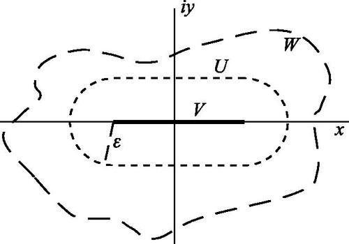
Let $V\subset W$, where V is a finite real closed interval and W is an open neighborhood of V in the complex numbers $\mathbb{C}$. Suppose the continuous function $f:\mathbb{R}\times W\to \mathbb{C}$ is complex analytic for all fixed t and that f(t, z) restricts on $\mathbb{R}\times V$ to a function f(t, x) determining a real-valued differential equation $x\prime =f(t,x)$. If the Poincaré map P(x) and thus the displacement map F(x) are defined for all x in V, it follows that the displacement map F(z) for the differential equation $z\prime =f(t,z)$ extends F(x) and that F(z) is defined and analytic on some ϵ-neighborhood U of V in $\mathbb{C}$ [7, p. 36], [22, p. 44] (see Figure 1). Ilyashenko applies to the displacement map F(z) his general theorem that gives an upper bound for the number of zeros on V of any function that is complex analytic in an ϵ-neighborhood U of V in $\mathbb{C}$ (Theorem 2).

Fig. 1 ϵ-neighborhood U of the closed interval V.

2.2 Jensen’s formula

Ilyashenko’s method is based on a novel application of Jensen’s formula, a result that was published in 1899 in Acta Mathematica as a letter from Jensen to Mittag-Leffler, the founder and editor of that distinguished journal [19]. This formula relates the position of the zeros of a function within a disk to the logarithm of its absolute value on the boundary of the disk. Accounts of how the foundations of complex analysis were understood at the time are found in [6, 10].

Johan Jensen was a Danish electrical engineer and amateur mathematician who never held an academic position. It is surprising and also gratifying that this outsider was able to conjecture and prove in a few lines an important result that had eluded some of the greatest mathematicians of the nineteenth century. We are informed in a biographical article on Jensen by Børge Jessen, himself a distinguished Danish mathematician, that Jensen was an admirer of Weierstrass [20]. This is evident in Jensen’s own proof of his formula [19], a proof based on power series methods. Such methods were preferred by Weierstrass and his followers. Jensen uses the term holomorphic, a term introduced by followers of Cauchy, but the term was sometimes also used by followers of Weierstrass [6, p. 718]. The result is stated and proved elegantly and correctly, as one would expect from Jessen’s remark that “his papers are patterns of exact and precise exposition” [20]. There is a great charm to Jensen’s letter. He begins by addressing Monsieur le Professeur and then chattily notes his attendance at some lectures recently given by the addressee. There is a buoyant enthusiasm throughout, from the title that announces a new and important result, to the hopes expressed at the end that his result will enable progress to be made on the Riemann conjecture regarding the zeros of the zeta function. While these hopes were not realized, Jensen’s formula was used extensively in succeeding investigations of entire functions; that is, functions holomorphic on the whole complex plane [1, p. 208].

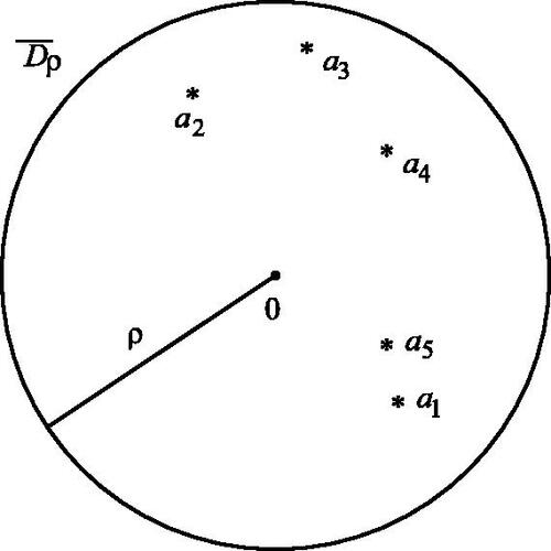
Jensen’s Formula ([1, p. 207], [28, p. 181])

Suppose f is holomorphic in the closed disk of radius ρ, f(0) is nonzero, and f has n zeros in the interior of the disk, counted with multiplicities, and these zeros occur at points $z=a_i$ (see Figure 2). Then $$\text{ln}\hspace{0.17em}|f(0)|=-\sum _{i=1}^n\hspace{0.17em}\text{ln}\hspace{0.17em}\left|\frac{\rho }{a_i}\right|+\frac{1}{2\pi }{\int }_0^{2\pi }\hspace{0.17em}\text{ln}\hspace{0.17em}|f(\rho e^{i\theta })|d\theta .$$

Fig. 2 Jensen’s formula: n = 5 zeros of f(z). Zeros located at $z=a_i$.

Proofs of Jensen’s formula rely on variations of the following procedure that cancels the zeros of f in the interior of the disk of radius ρ. Let $F(z)=f(z){\prod }_{i=1}^n\frac{{\rho }^2-\overline{a_i}z}{\rho (z-a_i)}$. Note that $F(0)\ne 0$. On the circle $\left|z\right|=\rho$, let $z=\rho e^{i\theta }$, and observe that for each term $\frac{{\rho }^2-\overline{a_i}z}{\rho (z-a_i)}$ the numerator and denominator have the same absolute value and so $\left|\frac{{\rho }^2-\overline{a_i}z}{\rho (z-a_i)}\right|=1$. Therefore $|F(z)|=|f(z)|$ on the circle $\left|z\right|=\rho$. We then take a branch of the complex logarithm of F(z). Jensen works with a power series representation that he integrates term by term about the circle [19], Saks and Zygmund directly apply the Cauchy integral theorem for a circle [28], while Ahlfors uses the result that $\text{ln}\hspace{0.17em}|F(z)|$ is a well-defined harmonic function on ${\mathbb{R}}^2$ and thus satisfies the mean value property for such functions [1, p. 165], a property that he previously establishes using the Cauchy integral theorem.

Ilyashenko relies on the following corollary to Jensen’s formula. As there are some subtle points, a proof of the corollary is given below.

Corollary to Jensen’s Formula

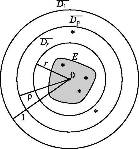
Suppose f is holomorphic in the open disk D₁ of radius 1 and continuous in the closed disk $\overline{D_1}$ of radius 1 and f(0) is nonzero. Let $M=\max \left\{\right|f(z)\left|\right|z\in \overline{D_1}\}$. Let E be a compact subset of the open disk D₁ that is contained in a closed disk $\overline{D_r}$ of radius r, with $0<r<1$. Let N be the number of zeros counted with multiplicity of f restricted to E (see Figure 3). Then:

Fig. 3 Corollary to Jensen’s formula: n = 5 zeros of f(z) at points marked by $*$; N = 3 zeros in compact subset E of $\overline{D_r}$.

1. $N\le \frac{1}{\hspace{0.17em}\text{ln}\hspace{0.17em}(1/r)}\text{ln}\hspace{0.17em}(\frac{M}{|f(0)|})$.

2. If $0\in E,m=\max \left\{\right|f(z)\left|\right|z\in E\}$, and $m=|f(0)|$, then $N\le \frac{1}{\hspace{0.17em}\text{ln}\hspace{0.17em}(1/r)}\text{ln}\hspace{0.17em}\left(\frac{M}{m}\right)$.

Proof.

(a) We can choose ρ arbitrarily close to 1 with $r<\rho <1$. f is holomorphic on the closed disk of radius ρ. Suppose f has n zeros in the interior of the disk of radius ρ, counted with multiplicity, and these zeros occur at points $z=a_i$. For all θ, $\rho e^{i\theta }$ is contained in $\overline{D_1}$ and thus $|f(\rho e^{i\theta })|\le M$. By Jensen’s formula, $\text{ln}\hspace{0.17em}|f(0)|\le -{\sum }_{i=1}^n\hspace{0.17em}\text{ln}\hspace{0.17em}\left|\frac{\rho }{a_i}\right|+\hspace{0.17em}\text{ln}\hspace{0.17em}(M)$ and therefore ${\sum }_{i=1}^n\hspace{0.17em}\text{ln}\hspace{0.17em}\left|\frac{\rho }{a_i}\right|\le \hspace{0.17em}\text{ln}\hspace{0.17em}(\frac{M}{|f(0)|})$. For each zero a_i of f that is contained in $E\subset \overline{D_r}$, we have $\left|a_i\right|\le r$ and thus $\text{ln}\hspace{0.17em}\left(\frac{\rho }{r}\right)\le \hspace{0.17em}\text{ln}\hspace{0.17em}\left|\right(\frac{\rho }{a_i}\left)\right|$. So $N\hspace{0.17em}\text{ln}\hspace{0.17em}\left(\frac{\rho }{r}\right)\le \hspace{0.17em}\text{ln}\hspace{0.17em}(\frac{M}{|f(0)|})$, for all ρ with $r<\rho <1$. Letting ρ approach 1, we obtain the desired conclusion.

(b) Part (b) follows by assuming that $m=|f(0)|$. □

2.3 Poincaré metric

The Poincaré metric is well-suited to studying complex analytic functions on the open unit disk D₁. A detailed treatment can be found in [21].

For the Poincaré metric, a differentiable curve C in the disk D₁, given by $z(t)=x(t)+iy(t)$ with $a\le t\le b$, has length determined by the integral$${\int }_a^b\frac{2\sqrt{{(x\prime (t))}^2+{(y\prime (t))}^2}}{1-{(x(t))}^2-{(y(t))}^2}dt,$$an integral that is often written invariantly as ${\int }_C\frac{2ds}{1-|z{|}^2}$. The distance $d(z_1,z_2)$ between two points in D₁ is defined by the infimum of the lengths of all curves connecting z₁ and z₂. The term Poincaré metric refers both to the distance $d(z_1,z_2)$ and to the function $\Delta (z)=\frac{2}{1-|z{|}^2}$. This function is sometimes called the metric density. Note that when defining the Poincaré metric some writers such as those of [21] divide by 2 the distance function and the metric density that are defined above.

The curve-lengths and distances are invariant under the fractional linear transformations $T(z)=\frac{az+b}{cz+d}$ that map the disk D₁ homeomorphically to itself. These fractional linear transformations are the isometries of the Poincaré metric.

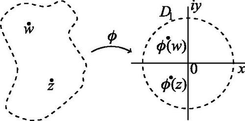
By using the Riemann mapping theorem, the Poincaré metric can also be defined on any open set U properly contained in $\mathbb{C}$ provided that U is homeomorphic to D₁. According to that justly celebrated theorem, the homeomorphism from U to D₁ can be chosen to be a complex analytic function $\varphi$. The distance $d_U(w,z)$ between two points in U can then be defined as $d(\varphi (w),\varphi (z))$ using the previous definition of the Poincaré metric on D₁ (Figure 4). The metric on U is well-defined because any two such complex analytic homeomorphisms ${\varphi }_1$ and ${\varphi }_2$ from U to D₁ differ by a fractional linear transformation T of D₁ (that is, ${\varphi }_1=T°{\varphi }_2$), and, as mentioned above, such transformations T are isometries of the Poincaré metric on D₁. Similarly, the Riemann map $\varphi$ from U to D₁ determines a positive real metric density ${\Delta }_U(z)=\varphi \prime (z)\Delta (\varphi (z))$ at each point z in U and the length of any curve C in U is given by ${\int }_C{\Delta }_U(z) ds$ [21]. If the curve is given parametrically by $z(t)=x(t)+iy(t)$ with $a\le t\le b$, then the length of C is determined by the integral ${\int }_a^b{\Delta }_U(z(t))\sqrt{{(x\prime (t))}^2+{(y\prime (t))}^2}dt$.

Fig. 4 Poincaré metric on an open set U homeomorphic to D₁.

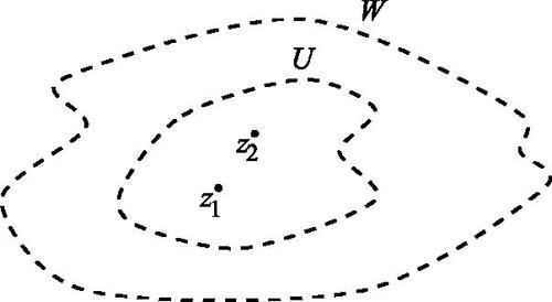
The inclusion principle is a fundamental property of the Poincaré metric. Let d_U and d_W be the Poincaré metrics as defined above on U and W, respectively, where U is contained in W and let Δ_U and Δ_W be the respective metric densities. Then for all z₁ and z₂ in U, we have $d_U(z_1,z_2)\ge d_W(z_1,z_2)$. Intuitively z₁ and z₂ are closer to the boundary of U than they are to the boundary of W, so their Poincaré distance in U is greater than their Poincaré distance in W (see Figure 5). Similarly, at all points z in U, we have ${\Delta }_U(z)\ge {\Delta }_W(z)$.

Fig. 5 The inclusion principle: $d_U(z_1,z_2)\ge d_W(z_1,z_2)$.

The Poincaré metric on an open disk of radius ϵ is an important special case for what follows. For $U=D_{ϵ}$, the open disk of radius ϵ centered at the origin, the Riemann map from U to D₁ is defined by $\varphi (z)=\frac{z}{ϵ}$. So ${\Delta }_U(z)=|\varphi \prime (z)|\Delta (\varphi (z))=\frac{1}{ϵ}\frac{2}{1-{(\frac{\left|z\right|}{ϵ})}^2}=\frac{2ϵ}{{ϵ}^2-|z{|}^2}$. Similarly, for any open disk U of radius ϵ centered at a point p in $\mathbb{C}$, we obtain ${\Delta }_U(z)=\frac{2ϵ}{{ϵ}^2-|z-p{|}^2}$.

3 Ilyashenko’s Theorems on Zeros and Periodic Solutions

In this section, we draw two theorems from Ilyashenko’s article [15]. These results place upper bounds on the number of zeros of a complex analytic function f on a compact set K contained in a domain U homeomorphic to the open unit disk. The section concludes with an application of Ilyashenko’s method to a differential equation arising from Hilbert’s sixteenth problem. Formula (6) in [15] should have a factor of 2 inside the exponential function and thus read $\gamma (U,K)\le \hspace{0.17em}\text{exp}\hspace{0.17em}(2K{ϵ}^{-1})$. The appropriate changes have been made throughout this article including in the statement of Theorem 3.

Theorem 1

([15]). For some domain U, assume there is a function $\varphi$ analytic on U that maps the closure $\overline{U}$ homeomorphically onto the closed disk $\overline{D_1}$. These conditions are satisfied if U is the interior of a Jordan curve. Let f be holomorphic on U and continuous on its closure $\overline{U}$, with $M=\max \left\{\right|f(z)\left|\right|z\in \overline{U}\}$. Let K be a compact subset of U, with $m=\max \left\{\right|f(z)\left|\right|z\in K\}$ such that $m\ne 0$. Let N be the number of zeros counted with multiplicity of f(z) restricted to K and let σ be the diameter of K in the Poincaré metric on U. Then:

1. For any r < 1 such that $\varphi (K)\subseteq \overline{D_r}$, we have $N\le \frac{1}{\hspace{0.17em}\text{ln}\hspace{0.17em}\left(\frac{1}{r}\right)}\text{ln}\hspace{0.17em}\left(\frac{M}{m}\right)$.

2. $N\le (e^{\sigma }-1)\hspace{0.17em}\text{ln}\hspace{0.17em}\left(\frac{M}{m}\right)$ for $\sigma \ge \hspace{0.17em}\text{ln}\hspace{0.17em}(2)$ and $N<\hspace{0.17em}\text{ln}\hspace{0.17em}\left(\frac{M}{m}\right)$ for $\sigma <\hspace{0.17em}\text{ln}\hspace{0.17em}(2)$.

3. $N\le e^{\sigma }\hspace{0.17em}\text{ln}\hspace{0.17em}\left(\frac{M}{m}\right)$.

Proof.

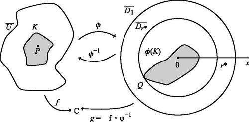
(a) For a proof that the interior of a Jordan curve satisfies the hypothesis of Theorem 1, see [30]. Choose a point P in K such that $|f(P)|=m=\max \left\{\right|f(z)\left|\right|z\in K\}\ne 0$. By composing if necessary with a fractional linear transformation T on $\overline{D_1}$, we can assume that $\varphi (P)=0$. The composition $g=f°{\varphi }^{-1}$ is holomorphic on the open disk D₁ of radius 1 and continuous on the closed disk $\overline{D_1}$ (see Figure 6) Then $M=\max \left\{\right|g(z)\left|\right|z\in \overline{D_1}\},m=\max \{|g(z)||z\in \varphi (K)\},m=g(0)\ne 0$, and N is the number of zeros counted with multiplicity of g restricted to $\varphi (K)$. The result follows by applying the corollary to Jensen’s formula to the function g and the compact set $\varphi (K)$.

Fig. 6 Theorem 1: P is in K, a compact subset of $\overline{U}$. $\varphi (K)\subseteq \overline{D_{r^{*}}}\subseteq \overline{D_1}$. $\varphi (P)=0$.

(b) If σ = 0, it follows that K contains only one point and that N = 0. The theorem follows trivially. Therefore, we will assume that $\sigma >0$.

As above, chose a point P in K such that $\varphi (P)=0$ and $|f(P)|=m=\max \left\{\right|f(z)\left|\right|z\in K\}\ne 0$. Because $\varphi$ is an isometry between the Poincaré metric on U and the Poincaré metric on D₁, σ is also the diameter of $\varphi (K)$ in the Poincaré metric on D₁. By the compactness of $\varphi (K)$, there is some closed disk with center 0 that contains $\varphi (K)$ and has a minimal radius $r^{*}$ with $0<r^{*}<1$; that is, $r^{*}=\min \left\{\nu \right|\varphi (K)\subseteq \overline{D_{\nu }}\}$ (Figure 6). By part (a), $N\le \frac{1}{\hspace{0.17em}\text{ln}\hspace{0.17em}\left(\frac{1}{r^{*}}\right)}\text{ln}\hspace{0.17em}\left(\frac{M}{m}\right)$. It remains to determine $r^{*}$ in terms of σ.

We observed above that 0 is in $\varphi (K)$. Furthermore, by the definition of $r^{*}$, there is a point Q in $\varphi (K)$ that lies on the boundary of the disk of radius $r^{*}$. Therefore, using the Poincaré metric on D₁ and its isotropy property,$$\sigma =\text{diameter of}\varphi (K)\ge d(0,Q)=d(0,r^{*})={\int }_0^{r^{*}}\frac{2}{1-x^2}dx=\hspace{0.17em}\text{ln}\hspace{0.17em}\left(\frac{1+r^{*}}{1-r^{*}}\right).$$

By elementary algebra and properties of the logarithm, for all $r^{*}$ with $0<r^{*}<1$, the inequality $\sigma \ge \hspace{0.17em}\text{ln}\hspace{0.17em}\left(\frac{1+r^{*}}{1-r^{*}}\right)$ is equivalent to the inequality $\text{ln}\hspace{0.17em}\left(\frac{e^{\sigma }+1}{e^{\sigma }-1}\right)\le \hspace{0.17em}\text{ln}\hspace{0.17em}\left(\frac{1}{r^{*}}\right)$. Therefore, $N\le \frac{1}{\hspace{0.17em}\text{ln}\hspace{0.17em}\left(\frac{e^{\sigma }+1}{e^{\sigma }-1}\right)}\text{ln}\hspace{0.17em}\left(\frac{M}{m}\right)$.

The inequality $\sigma \ge \hspace{0.17em}\text{ln}\hspace{0.17em}(2)$ implies $0<\frac{1}{e^{\sigma }-1}\le 1$. Using calculus, $\text{ln}\hspace{0.17em}(1+2x)\ge x$ for all x, $0\le x\le 1$. Therefore, for $\sigma \ge \hspace{0.17em}\text{ln}\hspace{0.17em}(2),\hspace{0.17em}\text{ln}\hspace{0.17em}\left(\frac{e^{\sigma }+1}{e^{\sigma }-1}\right)=\hspace{0.17em}\text{ln}\hspace{0.17em}(1+2(\frac{1}{e^{\sigma }-1}))\ge \frac{1}{e^{\sigma }-1}$, and so $N\le (e^{\sigma }-1)\hspace{0.17em}\text{ln}\hspace{0.17em}\left(\frac{M}{m}\right)$.

The inequality $0<\sigma <\hspace{0.17em}\text{ln}\hspace{0.17em}(2)$ implies $\text{ln}\hspace{0.17em}\left(\frac{e^{\sigma }+1}{e^{\sigma }-1}\right)>\hspace{0.17em}\text{ln}\hspace{0.17em}(3)>1$ and thus $N<\hspace{0.17em}\text{ln}\hspace{0.17em}\left(\frac{M}{m}\right)$.

(c) Part (c) follows directly from part (b). ■

Theorem 2

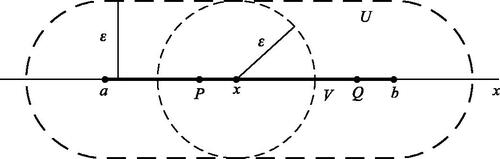
([15]). Let the “stadium” U be the open ϵ-neighborhood of a finite closed real interval $V=[a,b]$ of length L in the usual Euclidean metric and with diameter σ in the Poincaré metric on U (see Figure 7). Let f be holomorphic on U and continuous on its closure $\overline{U}$, with $M=\max \left\{\right|f(z)\left|\right|z\in \overline{U}\}$ and $m=\max \left\{\right|f(z)\left|\right|z\in V\}\ne 0$. Let N be the number of zeros counted with multiplicity of f(z) restricted to V. Then:

Fig. 7 Theorem 2: The diameter σ of V in the Poincaré metric on U equals $d_U(P,Q)$. As shown in the proof of Theorem 2, $d_U(P,Q)\le \frac{2L}{ϵ}$.

1. $\sigma \le \frac{2L}{ϵ}$.

2. $N\le \hspace{0.17em}\text{exp}\hspace{0.17em}\left(\frac{2L}{ϵ}\right)\hspace{0.17em}\text{ln}\hspace{0.17em}\left(\frac{M}{m}\right)$.

Proof.

(a) Since V is compact, the diameter σ of V equals the distance $d_U(P,Q)$ of two points P and Q in V (see Figure 7). This distance is at most equal to the Poincaré arclength along V between P and Q which is at most equal to the length L_U of V in the Poincaré metric on U. $L_U={\int }_a^b{\Delta }_U(x)dx$, where ${\Delta }_U(x)$ is the metric density of U evaluated at x. For each x between a and b, let $D_{ϵ}(x)$ be the open disk of radius ϵ centered at x, and let ${\Delta }_{ϵ,x}(z)=\frac{2ϵ}{{ϵ}^2-|z-x{|}^2}$ be the metric density for the Poincaré metric on $D_{ϵ}(x)$ (see Figure 7). Since $D_{ϵ}(x)$ is contained in U, by the inclusion principle we have ${\Delta }_U(z)\le {\Delta }_{ϵ,x}(z)$ for all z in $D_{ϵ}(x)$ (see Figure 5). Letting z = x, we have ${\Delta }_U(x)\le {\Delta }_{ϵ,x}(x)=\frac{2}{ϵ}$. Therefore,$$L_U={\int }_a^b{\Delta }_U(x)dx\le {\int }_a^b\frac{2}{ϵ}dx=\frac{2L}{ϵ},$$where $L=b-a$ is the usual Euclidean length of the interval V. So $\sigma \le L_U\le \frac{2L}{ϵ}$.

(b) Part (b) follows from part (a) and Theorem 1c. ■

3.1 Ilyashenko’s method

Consider a periodically forced differential equation $x\prime =f(t,x)$, where for all t, $f(t+T,x)=f(t,x)$. For convenience, we assume that the period T = 1. Upper bounds on the number of real periodic solutions of $x\prime =f(t,x)$ are determined by upper bounds on the number of zeros of the displacement map F. Using Theorem 2b, the method requires

1. a closed interval V containing the initial points of all real periodic solutions,

2. an ϵ-neighborhood U of V with closure $\overline{U}$ on which the displacement map F is defined and analytic,

3. the maximum M of $|F(z)|$ on the closure of U, and

4. the maximum m of $|F(z)|$ on V such that $m\ne 0$.

Using this method, Ilyashenko has obtained results pertinent to aspects of Hilbert’s sixteenth problem. For a survey, see [16]. Hilbert’s problem involves upper bounds on the number of limit cycles of polynomial planar differential equations, but a simplified version involves a one-dimensional equation of the form $x\prime =f(t,x)$ that is polynomial in x and periodic in t. Recall that a limit cycle is an attracting or repelling periodic solution. Charles Pugh inquired whether there was an upper bound on the number n of limit cycles that depended only on the degree d of the polynomial.

For d = 2, there are no more than two limit cycles. Furthermore, in the cubic case, for $x\prime =a_3(t)x^3+a_2(t)x^2+a_1(t)x+a_0(t)$ with the coefficient $a_3(t)$ of constant sign for all t, it was known that there could be no more than three limit cycles [3]. An important negative result was obtained by Lins Neto who showed that for any degree $d\ge 3$, and any n > 0, there is such an equation having at least n limit cycles [23]. In particular, in the cubic case d = 3, the constant sign condition on $a_3(t)$ is necessary to obtain the upper bound n = 3. However, it remained to determine upper bounds on n using not only the degree d but also properties of the coefficient functions of the polynomial.

Theorem 3

([15]). Suppose f(t, x) is of period 1 in t and polynomial of degree $d\ge 4$ in x with the x^d term having coefficient equal to 1 and where C > 1 is greater than the maximum of the absolute value of the coefficients of f. Then for the differential equation $x\prime =f(t,x)$ there is some number N(C, d), depending only on d and C, such that the number of limit cycles is at most N(C, d). Moreover, $$N(C,d)\le 8\hspace{0.17em}\text{exp}\hspace{0.17em}\{(6C+4)\hspace{0.17em}\text{exp}[(3/2){(2C+3)}^d\left]\right\}.$$

Stephen Smale has directed attention to the Liénard equation, another special case of Hilbert’s sixteenth problem [29]. By reducing the problem to a one-dimensional periodically forced equation and using a technique more elaborate but similar to that in the previous theorem, Ilyashenko and Panov obtained the following result:

Theorem 4

([17]). Consider the Liénard equation $$x\prime =y-F(x),y\prime =-x,F(x)=x^n+\sum _{j=1}^{n-1}{a}_j{x}^j,$$where $\left|a_j\right|\le C,C\ge 4,n\ge 5$, and n is odd. Then the number of limit cycles $L(n,C)\le \hspace{0.17em}\text{exp}\hspace{0.17em}(\hspace{0.17em}\text{exp}\hspace{0.17em}(C^{14n}))$.

The reason for the double or triple exponential character of these estimates will be suggested by the proofs of similar results in Section 5, results that apply Ilyashenko’s method to certain equations $x\prime =f(t,x)$ that arise from the neural model of Section 4 and for which f is transcendental in x.

Returning to the constant sign cubic case, suppose f(t, x) is qualitatively similar to functions $a_3(t)x^3+a_2(t)x^2+a_1(t)x+a_0(t)$ with $a_3(t)$ of constant sign for all t; that is, for all t there is one inflection point and no more than two turning points, and either for all t, $\underset{x\to \pm \infty }{\lim }f(t,x)=\pm \infty$, or for all t, $\underset{x\to \pm \infty }{\lim }f(t,x)=\mp \infty$. It was conjectured that as in the constant sign cubic case, the differential equation $x\prime =f(t,x)$ would have no more than three limit cycles. This conjecture was recently answered in the negative by Decker and Noonburg, with examples drawn from the neural model of Section 4 exhibiting an arbitrarily large number of limit cycles [8, 9].

4 Periodic Solutions of a Neural Model

4.1 Sigmoid response functions

In the simplest models, a neuron gives an all-or-nothing response to a stimulus; that is, the response is gated by a translate of the unit step function $u(x)=\{\begin{array}{cc}0\hfill & x<0\hfill \\ 1\hfill & x\ge 0\hfill \end{array}$. However, to use the resources of calculus and differential equations, it is preferable to have a response function S that rises smoothly from 0 to 1 as x passes from $-\infty$ to $\infty$. We normalize the model as follows.

Definition.

A sigmoid response function S is a continuously twice differentiable increasing function of the real numbers $\mathbb{R}$ that is concave up on $(-\infty ,0)$ and concave down on $(0,\infty )$ with $S(x)+S(-x)=1,S\prime (0)=1$, $\underset{x\to -\infty }{\lim }S(x)=0$, and $\underset{x\to \infty }{\lim }S(x)=1$.

In neural modeling, sigmoid response functions are often implemented using elementary functions. Four common examples are

1. $S(x)=\frac{1}{1+\hspace{0.17em}\text{exp}\hspace{0.17em}(-4x)},$

2. $S(x)=\frac{1}{\pi }\arctan (\pi x)+\frac{1}{2},$

3. $S(x)=\frac{1}{2}\tanh (2x)+\frac{1}{2},$

4. $S(x)=\frac{1}{2}\text{erf}\left(\sqrt{\pi }x\right)+\frac{1}{2}$, where the error function $\text{erf}(x)=\frac{2}{\sqrt{\pi }}{\int }_0^x\hspace{0.17em}\text{exp}\hspace{0.17em}(-t^2)dt.$

We plot $S(x)=\frac{1}{1+\hspace{0.17em}\text{exp}\hspace{0.17em}(-4x)}$ together with its bell-shaped derivative $S\prime (x)$ (see Figure 8).

Fig. 8 $S(x)=1/(1+\hspace{0.17em}\text{exp}\hspace{0.17em}(-4x)).$

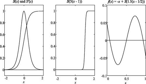
For any number r and for any k > 0, a transformation of S(x) yields the function $g(x)=S(k(x-r))$, with $g\prime (x)=kS\prime (k(x-r))$.The maximum value k of the derivative of this function g(x) occurs at its threshold x = r. For fixed r, as k approaches $\infty$, we see that g(x) approaches $u(x-r)$. This behavior is illustrated in the plot of $S(5(x-1))$ where $S(x)=\frac{1}{1+\hspace{0.17em}\text{exp}\hspace{0.17em}(-4x)}$ (Figure 8).

4.2 Neural models

The usual model for a single neuron is the four-dimensional Hodgkin–Huxley ordinary differential equation that led to the 1963 Nobel Prize in Physiology or Medicine for its discoverers. However, simpler models are easier to manipulate and may reveal important qualitative features of neural behavior. The two-dimensional Fitzhugh–Nagumo ordinary differential equation is such a simplification [24]. A further reduction yields an experimentally tested one-dimensional model derived from electrophysiological considerations [18, pp. 37, 55, 89, 106]. The model considered in this article shares qualitative features with this electrophysiological model [14], [25, pp. 78–80]. Furthermore, the model in this article has been applied successfully to the collective behavior of a single pool of neurons and of interacting pools of neurons including the much studied Wilson–Cowan oscillator [26, 31]. It is also used in differentiable artificial neural networks [13].

Let x represent the activation level of a neuron. Then x would decay exponentially if it were not for direct or indirect self-stimulation that is gated through a sigmoid response function S with threshold r and maximum derivative k. The resulting one-dimensional autonomous differential equation is $x\prime =f(x)=-x+S(k(x-r))$. We first discuss the qualitative features of this autonomous equation. We then discuss the periodically forced equation where the threshold r varies periodically.

For any sigmoid response function S, if $f(x)=-x+S(k(x-r))$ is the right-hand side of the differential equation, we obtain $f\prime (x)=0$ if and only if $S\prime (k(x-r))=1/k$. The bell-shaped properties of $S\prime$ imply that the equation $f\prime (x)=0$ has two solutions for k > 1, one solution for k = 1, and no solutions for k < 1. Therefore, f has at most three zeros, and the differential equation $x\prime =f(x)$ has at most three equilibria. As an example, we graph f using $S(x)=\frac{1}{1+\hspace{0.17em}\text{exp}\hspace{0.17em}(-4x)}$, k = 1.5, and r = 1/2 (Figure 8).

For the example above, at the equilibrium with the smallest x value and at the equilibrium with the largest x value, the derivative $f\prime <0$, implying that these equilibria are sinks or attractors; that is, solutions with initial conditions sufficiently close to such an equilibrium converge to the equilibrium as time t increases. At the middle equilibrium, the derivative $f\prime >0$, implying that this equilibrium is a source or repeller; that is, solutions with initial conditions sufficiently close to the equilibrium converge to the equilibrium as time t decreases and move away from the equilibrium as time t increases. It is this behavior that makes this equation a useful neural model, as neurons and neuron populations are often in either a low-activation state or in a high-activation state. Furthermore, because the derivative $f\prime$ is nonzero at each of the three equilibria, it follows for sufficiently small perturbations of f and $f\prime$ that the equilibria persist, respectively, as attractors and as a repeller [3], [5, pp. 84–89], [11]. In the language of dynamical systems theory, an equilibrium at which $f\prime$ is nonzero is called hyperbolic, and a differential equation $x\prime =f(x)$ such that the number and type of equilibria persist under sufficiently small perturbations of f and $f\prime$ is called structurally stable [12].

4.3 Periodic stimulation and periodic solutions

Abnormal oscillatory behavior of regions of the brain is characteristic both of epilepsy and Parkinson’s disease and is much studied and modeled [2]. Periodic stimulation of parts of the brain is increasingly used in the treatment of those cases of epilepsy that do not respond to medication [27]. Periodic stimulation of a single neuron or of a pool of neurons may come from other parts of the brain or from external sources. Periodic input into the one-variable neuron model is equivalent to a periodic change in the threshold r. Therefore, we consider the periodically stimulated nonautonomous one-dimensional ordinary differential equation model $x\prime =f(t,x)=-x+S(k(x-r(t)))$, where S is a sigmoid response function, k > 0, and r is continuous with period 1.

To be specific at this point, we consider a periodic perturbation of the autonomous equation discussed above: $x\prime =f(t,x)=-x+S(k(x-r(t)))$, where $S(x)=\frac{1}{1+\hspace{0.17em}\text{exp}\hspace{0.17em}(-4x)}$, k = 1.5, $r(t)=r_0+r_1(t)$, where $r_0=1/2$ and r₁ is continuous with period 1.

When the equilibria are hyperbolic, as in the unperturbed example, then for a sufficiently small magnitude perturbation r₁ about the threshold r₀, the three equilibria persist as three periodic solutions. The low and high excitation solutions are attractors and the middle solution is a repeller [3, 11], [26, pp. 1595–1598].

More generally, consider for this example the nullclines $f(t,x)=0$ and the generalized nullclines $f_x(t,x)=0$ [3, pp. 205–208]. For the unperturbed example, the nullclines are three horizontal lines $x=x_0,x=x_1$, and $x=x_2$ corresponding to the three equilibria x₀, x₁, and x₂, while the generalized nullclines are two horizontal lines $x=c_1$ and $x=c_2$ corresponding to the two critical points c₁ and c₂. For small enough perturbations, the nullclines persist as curves $x_0(t),x_1(t)$, and $x_2(t)$ in the (t, x)-plane that are not solutions of the differential equation, but rather indicate where the slope field of the differential equation is horizontal. If constants $d_1$ and d₂ exist with $x_0(t)<d_1<x_1(t)<d_2<x_2(t)$, then the differential equation has at least three periodic solutions. Furthermore, if $f_x(t,x)<0$ for $x<d_1$ and $x>d_2$ and $f_x(t,x)>0$ for $d_1<x<d_2$, then there are precisely three periodic solutions, with the low and high excitation solutions attractors and the middle solution a repeller [3, 11, 26].

These methods break down when the values of k and r become sufficiently large so that the nullclines are no longer separated by constants or no longer persist as three separate curves but rather have branches that join and separate in the interval $0\le t\le 1$. In such cases, the number of periodic solutions may be less than, equal to, or greater than three [3, 11, 26].

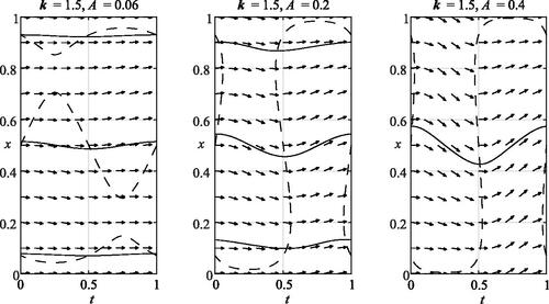
To be specific, consider the following example: $x\prime =f(t,x)=-x+S(k(x-r(t)))$, where $S(x)=\frac{1}{1+\hspace{0.17em}\text{exp}\hspace{0.17em}(-4x)}$, k = 1.5, $r(t)=r_0+r_1(t)$, where $r_0=1/2$ and $r_1(t)=A\hspace{0.17em}\text{sin}\hspace{0.17em}(2\pi t)$. As shown in Figure 9, for A = 0.06 the three nullclines are separated by constants and there are precisely three periodic solutions. For $A=0.2$, the nullclines no longer persist as separate curves, but there are still precisely three periodic solutions. For A = 0.4, the nullclines no longer persist as separate curves and there is only one periodic solution.

Fig. 9 Nullclines $f(t,x)=0$ (dashes), slope field, and periodic solutions (solid lines) for k = 1.5, r = 1/2, and A = 0.06, A = 0.2, and A = 0.4.

For the example above, the function f(t, x) seems qualitatively cubic-like (see the last paragraph of Section 3), that is, similar to a function $a_3(t)x^3+a_2(t)x^2+a_1(t)x+a_0(t)$ with the coefficient $a_3(t)$ negative for all t, and it was known that differential equations of the form $x\prime =a_3(t)x^3+a_2(t)x^2+a_1(t)x+a_0(t)$ with $a_3(t)$ of constant sign have no more than three periodic solutions [3]. So it was conjectured that differential equations from the neural model of the form $x\prime =f(t,x)$ also have no more than three periodic solutions.

This conjecture was answered in the negative by Decker and Noonburg who, using a careful bifurcation analysis, explored an example with five periodic solutions [8]. Such an example is provided by the equation $x\prime =f(t,x)=-x+S(k(x-r(t)))$, with $S(x)=\frac{1}{1+\hspace{0.17em}\text{exp}\hspace{0.17em}(-4x)}$, k = 3, $r(t)=r_0+r_1(t),r_0=1/2$, A = 0.37, and $r_1(t)=A\hspace{0.17em}\text{sin}\hspace{0.17em}(2\pi t)$.

Furthermore, by first studying examples where $k=\infty$ and r(t) is piecewise linear, and then smoothing these examples, Decker and Noonburg demonstrated that for any n > 0, there exist k > 0 and a continuous periodic function r, such that there are at least n periodic solutions for the equation $x\prime =f(t,x)=-x+S(k(x-r(t)))$ [9].

Many questions remain. One such is to find an upper bound N for the number of periodic solutions that is dependent on k and on S, but is independent of the perturbation r. In Section 5, we find an answer to such questions using complex analytic techniques developed by Yulij Ilyashenko.

5 Upper Bounds for Number of Periodic Solutions of Neural Models

Ilyashenko’s method finds upper bounds on the number of real periodic solutions of $x\prime =f(t,x)$ by finding upper bounds on the number of zeros of the displacement map F (see Section 2). The method requires (see Theorem 2)

1. a closed interval V containing the initial points of all real periodic solutions,

2. an ϵ-neighborhood U of V with closure $\overline{U}$ on which the displacement map F(z) is defined and analytic,

3. the maximum M of $|F(z)|$ on the closure of U, and

4. the maximum m of $|F(z)|$ on V such that $m\ne 0$.

For the periodically forced neuron of Section 4, these elements are established in Proposition 5. They are then used in Theorems 9 and 11 to obtain results on the number of real periodic solutions.

Recall that a function on a subset of $\mathbb{C}$ is defined to be complex analytic if it is complex analytic in some neighborhood of that subset [1]. Note that F may fail to be defined at a point z₀ in U if f is undefined at z₀, or if f fails to be complex analytic at z₀, or if the solution z(t) starting at z₀ fails to be defined for all t less than or equal to the period of the differential equation.

Definition.

A complex sigmoid response function S is a sigmoid response function that is complex analytic on the real line.

Definition.

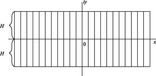
A complex sigmoid response function has (H, B) bounded derivative if $H>0$, B > 1, $S\prime$ is complex analytic in the closed H-neighborhood of the real axis, and for all z in that H-neighborhood we have $|S\prime (z)|\le B$ (see Figure 10).

Fig. 10 Definition: $S\prime$ is (H, B) bounded if $|S\prime (z)|\le B$ in the closed H-neighborhood of the real axis.

Proposition 5.

Let S be a complex sigmoid response function with (H, B) bounded derivative. Consider the differential equation $z\prime =f(t,z)=-z+S(k(z-r(t)))$, where $k\ge 1$ and r(t) is real-valued and continuous with period 1. Let V be the interval $[-1,1]$. Suppose $ϵ=H/(k{e}^{1+Bk})$, U is the ϵ-neighborhood of V, A is the closed $\frac{H}{k}$-neighborhood of V, P is the time-one (i.e., Poincaré) map, $F(z)=P(z)-z$ is the displacement function, $M=\max \left\{\right|F(z)\left|\right|z\in \overline{U}\}$, and $m=\max \left\{\right|F(z)\left|\right|z\in V\}$. Then:

1. V contains the initial points of all real periodic solutions of the differential equation.

2. On the closure of U, the Poincaré map P and the displacement function F are defined and analytic and P takes values in A.

3. $M\le 2(1+\frac{H}{k})$.

4. $m\ge 1-\frac{1}{e}$.

Proof.

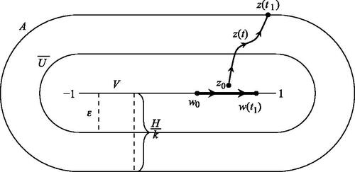
Note that the three lemmas included in the proof of Proposition 5 are only used for the proof of part (b).

1. Consider a solution x(t) with initial condition x₀. The bounds on S, $0<S(k(z-r(t)))<1$, imply $f(t,x)>0$ for x < 0 and $f(t,x)<0$ for x > 1. If $x_0<0$, then there is a neighborhood of x₀, such that, for all t, x(t) is increasing while in that neighborhood, showing that x(t) is not a periodic solution. Similarly, x(t) is not a periodic solution whenever $x_0>1$. Therefore, the closed unit interval and hence V contain all initial points for all periodic solutions.

2. Note that $\overline{U}\subseteq A$ and that, by the assumption $k\ge 1$, A is a subset of the closed H-neighborhood of the real axis. Therefore the functions f(t, z) and $f_z(t,z)$ are defined for all (t, z) with z in A, as is the differential equation $z\prime =f(t,z)=-z+S(k(z-r(t)))$. Suppose z₀ is in the closure of U and let z(t) be the solution of $z\prime =f(t,z)=-z+S(k(z-r(t)))$ with initial condition $z(0)=z_0$. We need to show that z(t) is defined and in A for all $t\le 1$ (see Figure 11). Suppose not. We use the following three lemmas to derive the contradiction $\frac{H}{k}<\frac{H}{k}$. Lemma 7 is a corollary of Gronwall’s inequality and is much used in the theory of differential equations.

   Fig. 11 Proposition 5b: On the closure of U, both the Poincaré map P and the displacement function F are defined and the Poincaré map takes values in A. The proof is by contradiction.

   

Lemma 6.

Let $D=\max \left\{\right|f_z(t,z)\left|\right|t\in \mathbb{R},z\in A\}$. For all fixed t and all points P and Q in A, $|f(t,P)-f(t,Q)|\le D|P-Q|$; i.e., for all fixed t, D is a Lipschitz constant in z for f(t, z) on A.

Proof.

Note that the maximum D exists since f is periodic in t and A is compact. Since A is convex, the straight-line path C from P to Q lies in A.$$|f(t,P)-f(t,Q|=\left|{\int }_C{f}_z(t,z)dz\right|\le {\int }_C|f_z(t,z)|\left|dz\right|\le D|P-Q|.$$

See [1, p. 104]. □

Lemma 7.

([4, p. 103], [12, pp. 169, 297]). For some $T\ge 0$, suppose $z_1(t)$ and $z_2(t)$ are solutions of $z\prime =f(t,z)$ that are contained in A for all t with $0\le t\le T$, and that for all fixed t, D is a Lipschitz constant in z for f(t, z) in A. Then $|z_2(t)-z_1(t)|\le |z_2(0)-z_1(0)|e^{Dt}$ for all t with $0\le t\le T$.

Lemma 8.

Let $D=\max \left\{\right|f_z(t,z)\left|\right|t\in \mathbb{R},z\in A\}$. Then $D\le 1+Bk$.

Proof.

If z is in the closed $\frac{H}{k}$-neighborhood A of V, then $|\text{Im}(z)|\le \frac{H}{k}$. Moreover, $|\text{Im}(z-r(t))|\le \frac{H}{k}$ because r is real-valued. So $|\text{Im}(k(z-r(t))|\le H$, which implies $|S\prime (k(z-r(t))|\le B$, because S has an (H, B) bounded derivative. Therefore, for all z in A, $|f_z(t,z)|=|-1+kS\prime (k(z-r(t))|\le 1+|kS\prime (k(z-r(t))|\le 1+Bk$. ■

Now suppose that there exists some $t\le 1$, such that either z(t) is not defined or that z(t) is defined but it is not in A. In either case there exists $t_1<1$, such that $z(t_1)$ is on the boundary of A and z(t) is in A for all $t\le t_1$. The distance from $z(t_1)$ to V is $\frac{H}{k}$ (Figure 11).

Choose a point w₀ in V such that $|z_0-w_0|\le ϵ$ and let w(t) be the solution of $z\prime =f(t,z)=-z+S(k(z-r(t)))$ with initial condition $w(0)=w_0$ (Figure 11). As argued in the proof of part (a), $f(t,x)>0$ for x < 0 and $f(t,x)<0$ for x > 1. Therefore, for all $t\ge 0$, w(t) is defined and in V and consequently in A. $z(t_1)$ on the boundary of the $\frac{H}{k}$ neighborhood A of V implies $\frac{H}{k}\le |z(t_1)-w(t_1)|$.

Since $t_1<1$, it follows by Lemmas 6, 7, 8 that$$\begin{array}{c}\frac{H}{k}\le |z(t_1)-w(t_1)|\le |z(0)-w(0)|e^{D{t}_1}\\ <|z(0)-w(0)|e^D\le |z(0)-w(0)|e^{1+Bk}.\end{array}$$

By choice of w(0), $|z(0)-w(0)|\le ϵ=H/(k{e}^{1+Bk})$, implying the contradiction $\frac{H}{k}<\frac{H}{k}$. Therefore, for all $t\le 1$, z(t) is defined and in A. In particular, for all z₀ in the closure of U, the Poincaré map $P(z_0)=z(1)$ is defined and in A.

It remains to show that the Poincaré map P and the displacement function F are complex analytic on the closure of U. The assumption $k\ge 1$ implies that $S\prime$ and thus also S are complex analytic on an open neighborhood W of A. Therefore, for all fixed t, the function $f(t,z)=-z+S(k(z-r(t)))$ is complex analytic on W. We have just shown that solutions with initial conditions in the closure of U remain in A and thus in W for all $t\le 1$. It follows from classical results on the analyticity of solutions with respect to initial conditions that the Poincaré function P and thus also the displacement function $F(z)=P(z)-z$ are complex analytic on the closure of U [22, p. 44].

1. By part (b), z in $\overline{U}$ implies P(z) in A. The real line is invariant for P, so either z and P(z) are both in the closed upper half of A or they are both in the closed lower half of A. Therefore, M is at most equal to the diameter of the closed upper half of A. This region is formed by a rectangle of length 2 and height $\frac{H}{k}$ together with quarter circles of radius $\frac{H}{k}$ at each end (Figure 11). The region has diameter $2(1+\frac{H}{k})$.

2. To find a lower bound for m we estimate $|x(1)-x(0)|$ from below, where we choose x(t) to be the solution of the differential equation $x\prime =f(t,x)=-x+S(k(x-r(t)))$ with initial condition $x(0)=-1$. For comparison, consider the exponential differential equation $x\prime =h(x)=-x$, with initial condition $x(0)=-1$ and solution $-e^{-t}$. Since for all x < 0, $f(t,x)>h(x)>0$, it follows that for all $t\ge 0,x(t)>-e^{-t}$. Therefore $m\ge |x(1)-x(0)|=x(1)-x(0)>\frac{-1}{e}-(-1)=1-\frac{1}{e}$. ■

We now apply Ilyashenko’s Theorem 2 using the estimates in Proposition 5.

Theorem 9.

Let S be a complex sigmoid response function with (H, B) bounded derivative. Let N be the number of real periodic solutions for the differential equation $z\prime =f(t,z)=-z+S(k(z-r(t)))$, where k > 0 and r(t) is real valued and continuous with period 1. Then:

1. $N\le \hspace{0.17em}\text{exp}\hspace{0.17em}\left(\frac{4k{e}^{1+Bk}}{H}\right)\hspace{0.17em}\text{ln}\hspace{0.17em}(\frac{2e(1+\frac{H}{k})}{e-1})$.

2. If $k\ge H$, then $N\le 2\hspace{0.17em}\text{exp}\hspace{0.17em}(Ck{e}^{Bk})$, where $C=4e/H$.

Proof.

(a) Suppose $k\ge 1$. By Proposition 5a, N equals the number of zeros of the displacement function F(z) on the interval $V=[-1,1]$. Under the assumptions of Theorem 2, $N\le \hspace{0.17em}\text{exp}\hspace{0.17em}\left(\frac{2L}{ϵ}\right)\hspace{0.17em}\text{ln}\hspace{0.17em}\left(\frac{M}{m}\right)$, where L = 2 is the length of V. By Proposition 5b, these assumptions are satisfied by $ϵ=H/(k{e}^{1+Bk})$. By parts (c) and (d) of Proposition 5, we estimate $M\le 2(1+\frac{H}{k})$ and $m\ge 1-\frac{1}{e}$. Substituting in $N\le \hspace{0.17em}\text{exp}\hspace{0.17em}\left(\frac{2L}{ϵ}\right)\hspace{0.17em}\text{ln}\hspace{0.17em}\left(\frac{M}{m}\right)$, we obtain the result.

If $0<k<1$, then for real x, $f_x(t,x)<0$ for all t, which yields the bound $0<P\prime (x)<1$ for the derivative of the Poincaré map P [3, pp. 109–110], [11, p. 130]. Therefore the displacement map $F(x)=P(x)-x$ is monotone decreasing and has at most one zero, implying that there is at most one periodic solution.

(b) Suppose $k\ge H$; then we have$$N\le \hspace{0.17em}\text{exp}\hspace{0.17em}\left(\frac{4k{e}^{1+Bk}}{H}\right)\hspace{0.17em}\text{ln}\hspace{0.17em}\left(\frac{4e}{e-1}\right)<2\hspace{0.17em}\text{exp}\hspace{0.17em}\left(\frac{4e}{H}k{e}^{Bk}\right).$$

6 Explicit Upper Bound on the Number of Periodic Solutions

In this section, we consider the complex sigmoid response function $S(z)=\frac{1}{1+\hspace{0.17em}\text{exp}\hspace{0.17em}(-4z)}$ from Section 4, and letting B = 2 we determine an explicit value of H such that the derivative $S\prime (z)$ is (H, B) bounded. We then use Theorem 9 to put an upper bound on the number N of real periodic solutions for the differential equation $z\prime =f(t,z)=-z+S(k(z-r(t)))$, where $k>0$ and r is real-valued with period 1. The value of H is determined by the magnitude of $S\prime$ near the real axis and, therefore, influenced by the location of the poles of S near the real axis.

Proposition 10

. $S(z)=\frac{1}{1+\hspace{0.17em}\text{exp}\hspace{0.17em}(-4z)}$ has (H, B) bounded derivative $S\prime (z)$ where $H=\frac{\pi }{8}$ and B = 2.

Proof.

The derivative $S\prime (z)=\frac{4e^{4z}}{{(1+e^{4z})}^2}$. The following statements are equivalent:

1. $|S\prime (z)|\le 2$,

2. $\left|{(e^{2z}+e^{-2z})}^2\right|\ge 2$,

3. $|{\cosh }^2(2z)|\ge 1/2$, and

4. ${\cosh }^2(2x)-{\hspace{0.17em}\text{sin}\hspace{0.17em}}^2(2y)\ge 1/2$, where $z=x+iy$.

This last inequality is satisfied for all x and y with $\left|y\right|\le \frac{\pi }{8}$. ■

As an exercise, using properties of elementary complex analytic functions, similar estimates can be obtained for the other examples of sigmoid response functions that are listed in Section 4.

Exercise. $S\prime (z)$ is (H, B) bounded with:

B = 2 and $H=\frac{\sqrt{2}}{2\pi }$, for $S(z)=\frac{1}{\pi }\arctan (\pi x)+\frac{1}{2}$,

B = 2 and $H=\frac{\pi }{6}$, for $S(z)=\frac{1}{2}\tanh (2z)+\frac{1}{2}$, and

B = 2 and $H=\sqrt{\frac{\hspace{0.17em}\text{ln}\hspace{0.17em}(2)}{\pi }}$, for $S(z)=\frac{1}{2}\text{erf}\left(\sqrt{\pi }x\right)+\frac{1}{2}$.

Theorem 11.

Let N be the number of real periodic solutions to the differential equation $z\prime =f(t,z)=-z+S(k(z-r(t)))$, where k > 0, r is real-valued and continuous with period 1, and $S(z)=\frac{1}{1+\hspace{0.17em}\text{exp}\hspace{0.17em}(-4z)}$. Then $N<2\hspace{0.17em}\text{exp}\hspace{0.17em}(Ck{e}^{2k})$ where $C=\frac{32e}{\pi }\approx 28$, approximating to the least integer larger than C.

Proof.

If $k\ge H=\frac{\pi }{8}$, Theorem 11 follows by applying Theorem 9b, using B = 2 and the value $H=\frac{\pi }{8}$ determined in Proposition 10. If $k<H=\frac{\pi }{8}<1$, then for real x, $f_x(t,x)<0$ for all t, which yields the bound $0<P\prime (x)<1$ for the derivative of the Poincaré map P [3, pp. 109–110], [11, p. 130]. Therefore the displacement map $F(x)=P(x)-x$ is monotone decreasing and has at most one zero, implying that there is at most one periodic solution. ■

7 Conclusions and Open Questions

After an introductory course in differential equations and an introductory course in complex analysis, the method of Ilyashenko can be used to study other accessible and illuminating problems involving upper bounds on the number of real periodic solutions of equations of the form $x\prime =f(t,x)$, where f is periodic in t and complex analytic in x. Delicate work is required to understand the particular function f and its derivative $f\prime$ and how these determine the elements of the approach (see Section 5).

For example, undergraduates may wish to consider the autonomous population model $x\prime =f(x)=rx(1-x/L)(x/M-1)-H$, where r is the intrinsic growth/decay rate, L is the carrying capacity, M is the minimal sustainable population in the absence of harvesting, H is the harvesting rate, and where r, L, and M are assumed to be positive with M < L [3, p. 217]. If H = 0, there are three equilibria: x = 0, x = L, and x = M. For small continuous periodic perturbations of the constants, the three equilibria persist as periodic solutions. Furthermore, whatever their size, as long as the periodic perturbations r(t), L(t), and M(t) remain positive, the coefficient of x³ remains of constant negative sign, and this implies that there can be no more than three periodic solutions. If r is allowed to vary in sign, one may search for examples with more than three periodic solutions, and then use Ilyashenko’s method to determine upper bounds on the number of such solutions.

Even for the neural models studied in this article, better estimates might be obtained by setting $V=[-c,1]$, for c > 0, and allowing B to approach 1 and c to approach 0.

Ilyashenko believes that the double or triple exponential estimates are likely to be far too big [15, 17]. He quotes Smale’s conjecture for the Liénard equation, that the number of periodic solutions is likely to be polynomial in d and independent of the magnitude C of the coefficients. Ilyashenko suggests that sharper estimates might be found by complexifying time t and studying the resulting foliations that have Riemann surfaces as leaves.

The estimate from Theorem 11 that $N<2\hspace{0.17em}\text{exp}\hspace{0.17em}(Ck{e}^{2k})$, with $C=\frac{32e}{\pi }$, suggests a very large number of periodic solutions that could not possibly be detected in either natural or artificial neural networks. However, this upper bound is independent of the periodic stimulation r and suggests the existence of a more plausible upper bound that cannot yet be theoretically demonstrated. Furthermore, seemingly impractical mathematical idealizations often find unexpected applications.

We conclude with three questions suggested by these studies. The last question is vague and requires further precision.

Question 1. Suppose a complex sigmoid response function S is complex analytic in some neighborhood of fixed width about the real axis. Does such an S have a derivative $S\prime$ that is (H, B) bounded for some H > 0 and B > 1?

Question 2. The piecewise linear function $L(x)=\{\begin{array}{cc}0,& x<-1/2\\ x+1/2,& -1/2\le x\le 1/2\\ 1,& x \ge 1/2\end{array}$has derivative $L\prime (0)=1$. Replace S(x) by L(x) in the neural model we have studied. Using real variable methods find an upper bound N for the number of periodic solutions to $x\prime =f(t,x)=-x+L(k(x-r(t)))$, where k > 0 and r is continuous and has period 1 in t. Using such methods can one obtain an estimate comparable to or better than the estimates in Theorem 11? To begin, consider the case $r(t)=\frac{1}{2}+A\hspace{0.17em}\text{sin}\hspace{0.17em}(2n\pi t)$ for n an integer starting with n = 1.

Question 3. For $x\prime =f(t,x)=-x+S(k(x-r(t)))$, for a fixed number k > 0 and a fixed complex sigmoid response function S, let N(k, S) be the supremum of the number of periodic solutions, where the supremum is taken over the set of continuous functions r with period 1. Note that Theorem 11 gives an estimate for N(k, S), where $S(x)=\frac{1}{1+\hspace{0.17em}\text{exp}\hspace{0.17em}(-4x)}$. Let N(k) be the infimum of N(k, S) where the infimum is taken over the set of complex sigmoid response functions S. What is the “best” upper estimate for N(k) that can be obtained using Ilyashenko’s method and (H, B) bounded derivatives as in Section 5?

ACKNOWLEDGMENT

This article was inspired by discussions I had with my University of Hartford colleagues Robert Decker, Virginia W. Noonburg, and Ben Pollina. Valuable suggestions were offered by Linda Keen, Malgorzata Marciniak, John Mitchell, and Zbigniew Nitecki. Nine of the figures were rendered by Andrew Starnes who used the LATEXpackage PGFPlots. Figures 8 and 9 were generated with Matlab. The meticulous work of the editors and reviewers was of great help and is much appreciated.

Additional information

Notes on contributors

Diego M. Benardete

Diego Mair Benardete received his doctorate in mathematics from the City University of New York in 1985 and has ever since researched pure and applied aspects of dynamical systems and differential equations. At the University of Hartford, he enjoys teaching undergraduate mathematics. He also has an amateur’s interest in history, literature, philosophy, and religion that manifests itself professionally in the study of the history and philosophy of mathematics.

References

- Ahlfors, L. (1979). Complex Analysis: An Introduction to the Theory of Analytic Functions of One Complex Variable, 3rd ed. New York, NY: McGraw-Hill.
- Ashwin, P., Coombes, S., Nicks, R. (2016). Mathematical frameworks for oscillatory network dynamics in neuroscience. J. Math. Neurosci. 6: Art. 2, 92 pp.
- Benardete, D., Noonburg, V. W., Pollina, B. (2008). Qualitative tools for studying periodic solutions and bifurcations as applied to the periodically harvested logistic equation. Amer. Math. Monthly. 115(3): 202–219.
- Birkhoff, G., Rota, G-C. (1962). Ordinary Differential Equations. Waltham, MA: Ginn and Company.
- Blanchard, P., Devaney, R. L., Hall, G. R. (1998). Differential Equations. Pacific Grove, CA: Brooks/Cole.
- Bottazini, U., Gray, J. (2013). Hidden Harmony—Geometric Fantasies: The Rise of Complex Function Theory. New York: Springer.
- Coddington, E. A., Levinson, N. (1985). Theory of Ordinary Differential Equations. Malabar, FL: Krieger. Reprint of original edition, (1955). New York, NY: McGraw-Hill.
- Decker, R., Noonburg, V. W. (2012). A periodically forced Wilson–Cowan system with multiple attractors. SIAM J. Math. Anal. 44(2): 887–905.
- Decker, R., Noonburg, V. W. A single neuron equation with multiple periodic cycles. In preparation.
- Gray, J. (2015). The Real and the Complex: A History of Analysis in the 19th Century. New York, NY: Springer.
- Hale, J. K., Kocak, H. (1991). Dynamics and Bifurcations. New York, NY: Springer.
- Hirsch, M. W., Smale, S. (1974). Differential Equations, Dynamical Systems, and Linear Algebra. Orlando, FL: Academic Press.
- Hopfield, J. J. (1982). Neural networks and physical systems with emergent collective computational abilities. Proc. Nat. Acad. Sci. 79: 2554–2558. DOI: https://doi.org/10.1073/pnas.79.8.2554.
- Hoppensteadt, F. C., Izhikevich, E. (1997). Weakly Connected Neural Networks. New York, NY: Springer.
- Ilyashenko, Yu. (2000). Hilbert-type numbers for Abel equations, growth and zeros of holomorphic functions. Nonlinearity. 13(4): 1337–1342. DOI: https://doi.org/10.1088/0951-7715/13/4/319.
- Ilyashenko, Yu. (2002). Centennial history of Hilbert’s 16th problem. Bull. Amer. Math. Soc. (N.S.). 39(3): 301–354.
- Ilyashenko, Yu., Panov, A. (2001). Some upper estimates of the number of limit cycles of planar vector fields with an application to the Liénard equations. Moscow Math. J. 1(4): 583–599. DOI: https://doi.org/10.17323/1609-4514-2001-1-4-583-599.
- Izhikevich, E. (2007). Dynamical Systems in Neuroscience: The Geometry of Excitability and Bursting. Cambridge, MA: MIT Press.
- Jensen, J. (1899). Sur un nouvel et important théorème de la théorie des fonctions. Acta. 22: 359–364. DOI: https://doi.org/10.1007/BF02417878.
- Jessen, B. (1973). Jensen, Johan Ludwig William Valdemar. In: Gillispie, C. C., ed. Dictionary of Scientific Biography, Vol. 7. New York: Scribner, p. 101.
- Keen, L., Lakic, N. (2007). Hyperbolic Geometry from a Local Viewpoint. New York: Cambridge Univ. Press.
- Lefschetz, S. (1963). Differential Equations: Geometric Theory, 2nd ed. New York: John Wiley.
- Lins Neto, A. (1980). On the number of solutions of the equation dxdt=∑0naj(t)xj,0≤t≤1, for which x(0)=x(1) . Invent. Math. 59(1): 67–76.
- Murray, J. D. (1993). Mathematical Biology, 2nd ed. New York, NY: Springer.
- Noonburg, V. W. (2019). Differential Equations: From Calculus to Dynamical Systems, 2nd ed. Providence, RI: MAA Press.
- Noonburg, V. W., Benardete, D., Pollina, B. (2003). A periodically forced Wilson–Cowan system. SIAM J. Appl. Math. 63(5): 1585–1603.
- Rolston, J. D., Eaglot, D. J., Wang, D, D., Shih, T., Chang, E. F. (2012). Comparison of seizure control outcomes and the safety of vagus nerve, thalamic deep brain, and responsive neurostimulation: evidence from randomized control trials. Neurosurg. Focus. 32(3): E14.
- Saks, S., Zygmund, A. (1971). Analytic Functions. Amsterdam: Elsevier.
- Smale, S., (1998). Mathematical problems for the next century. Math. Intelligencer. 20: 7–15. DOI: https://doi.org/10.1007/BF03025291.
- Veech, W. A. (1967). A Second Course in Complex Analysis. New York: W. A. Benjamin.
- Wilson, H. R., Cowan, J. D. (1972). Excitatory and inhibitory interactions in localized populations of model neurons. Biophys. J. 12: 1–24. DOI: https://doi.org/10.1016/S0006-3495(72)86068-5.