
 ?Mathematical formulae have been encoded as MathML and are displayed in this HTML version using MathJax in order to improve their display. Uncheck the box to turn MathJax off. This feature requires Javascript. Click on a formula to zoom.
Abstract
The classical produces wonderful infinite sequences of arithmetic and geometric means with common limit. For finite fields
with
we introduce a finite field analogue
that spawns directed finite graphs instead of infinite sequences. The compilation of these graphs reminds one of a jellyfish swarm, as the 3D renderings of the connected components resemble jellyfish (i.e., tentacles connected to a bell head). These swarms turn out to be more than the stuff of child’s play; they are taxonomical devices in number theory. Each jellyfish is an isogeny graph of elliptic curves with isomorphic groups of
-points, which can be used to prove that each swarm has at least
jellyfish. This interpretation also gives a description of the class numbers of Gauss, Hurwitz, and Kronecker which is akin to counting types of spots on jellyfish.
1 Arithmetic and geometric means
Beginning with positive real numbers and
the
inductively produces a sequence of pairs
consisting of arithmetic and geometric means. Namely, for
we let
For we have the elementary inequality
At a deeper level, the classical theory of the
(for example, see Chapter 1 of [Citation3]) establishes that these rapidly converging sequences have a common limit
In 1748, Euler [Citation3] employed as a remarkable device for rapidly computing digits of
Namely, he showed that
where
Although the first three terms are quite satisfying, the next two terms
are even more astounding as they give 11 and 20 decimal places of π respectively.
Is there a finite field analogue of If so, what number theoretic secrets does it reveal? The nonexistence of many square-roots in
poses an obvious obstacle. One solution would be to consider a process where the finite fields grow in size, allowing for the existence of square-roots. However, a second issue arises. Namely, what defines the correct choice of square-root? Over
the convention of taking positive square-roots guarantees that
never ventures beyond
Consequently, over finite fields we seek situations where there are unique choices of square-root that similarly avoid the need for field extensions.
These requirements hold for finite fields , where
with p prime. These fields enjoy the property that –1 is not a square, which corresponds to the fact that
is not a real number. For such a field
we let
be its quadratic residue symbol (the usual Legendre symbol
when q = p is prime). We then define
for pairs
with
and
This input data gives
and
and for
we let
(1.1)
(1.1) where bn is the unique square-root with
Although
has two square-roots, only one choice satisfies
as
. Therefore, we obtain a sequence of pairs
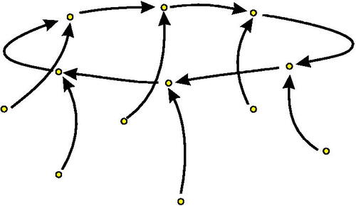
Let’s consider the case of Half of the 12 pairs that appear in some
form a single
-orbit
.
(Note. The overlined pairs form a repeating orbit.). The other 6 pairs lead to this orbit after a single step. For example, we have(1.2)
(1.2)
The compilation of all such sequences forms a connected directed graph ().
Fig. 1 3D rendering of .
This example is typical. The compilation of the sequences is always a disjoint union of connected directed graphs. The nodes are admissible ordered pairsFootnote1
where
with
and
Moreover,
is an edge if and only if
and
with
These connected components are like jellyfish, as their 3D renderings turn out to be unit length tentacles leading to a bell head cycle. Hence, we playfully refer to the compilation of the
sequences
(1.3)
(1.3) as the jellyfish swarm for
where the
are the individual jellyfish which make up the swarm.
Let’s summarize some basic facts about and the jellyfish swarms
Theorem 1.
If is a finite field with
then the following are true.
The
algorithm is well-defined.
The jellyfish swarm
Every jellyfish has a bell head with length one tentacles pointing to each node.
If
Proof of Theorem 1.
If (a, b) is admissible, then we must show that the next pair (c, d) generated by
We compute the number of admissible pairs (a, b). There are q – 1 choices for a, and
Each
Each
Theorem 1
inspires many natural questions. For example, how small (resp. large) are the jellyfish in a general swarm? This appears to be a very difficult question. For instance, there are -orbits that are much shorter than q, such as the length 9
as well as those that are much longer than q, such as the length 410
These examples correspond to a tiny 18 node jellyfish in , and a gigantic 820 node jellyfish in
As another question, what can be said about
the number of jellyfish in
? illustrates the oscillatory behavior of
This erratic sequence does not appear to settle into a predictable pattern as
Indeed, there are many astonishing examples of disproportionate consecutive values, such as
and
The only clear observation is that the
grow rapidly with m when p is fixed. For instance, we have
Table 1 for pimes q.
We shall see that the theory of elliptic curves offers deep insight into these questions.
2 Jellyfish swarms organize elliptic curves
Computing arithmetic and geometric means over might seem like mere child’s play. However, it turns out that this arithmetic process is a taxonomical device in number theory which organizes elliptic curves.
An elliptic curve E over a field can be thought of as a cubic equation of the form
where
and f has nonzero discriminant. If
denotes the
-rational points of E, including the identity “point at infinity” O, then
naturally forms an abelian group via the well-known “chord-tangent law.” The group law can be described by asserting that three colinear points on an elliptic curve sum to the identity O. Number theorists are deeply interested in these groups of rational points.
If F is a number field (i.e., a field which has finite degree over ), then a classical theorem by Mordell and Weil asserts that
the Mordell-Weil group of
, is finitely generated. The special case where
is the subject of two frequently cited Monthly articles. The beautiful 1993 article by Silverman [Citation17] on the representation of positive integers as sums of two rational cubes describes the intimate relationship between Ramanujan’s taxi-cab numbers and positive rank elliptic curves (i.e., curves with infinitely many
-rational points). The famous 1991 article by Mazur [Citation12] promotes the conjectured “Modularity” of elliptic curves over
(formerly known as the Taniyama-Weil Conjecture). This conjecture is now known to be true, largely thanks to the work of Wiles and Taylor [Citation20, Citation23], which was a celebrated ingredient in the proof of Fermat’s Last Theorem.
For the case of finite fields, it turns out that the jellyfish swarms organize elliptic curves. One can think of the nodes as spots on the jellyfish, and these spots will be mapped to curves. These swarms are coverings of networks of special Legendre elliptic curves when
and
To be precise, for
we recall the Legendre normal form elliptic curve
(2.1)
(2.1)
Isomorphism classes of elliptic curves are distinguished by their j-invariants, and for we have
(2.2)
(2.2)
For an introduction to elliptic curves over finite fields, the reader may consult Chapter 4 of [Citation22].
The jellyfish swarm organizes elliptic curves via the map
where
is the set of Legendre curves over
and
(2.3)
(2.3) where
For instance, (1.2) gives
As the values cover the squares in
it is natural ask what special features are shared by curves of the form
It turns out that these curves are distinguished by the 2-Sylow subgroups of their
-rational points.
Lemma 2.
Suppose that is a finite field with
If
then the 2-Sylow subgroup of
is of the form
where
Proof of Lemma 2.
Elliptic curves with four 2-torsion points (i.e., including the identity) can be written in the form
The nontrivial 2-torsion points correspond to the roots of the cubic. They are the points and
For such curves, the classical 2-descent lemma (see pp. 47–49 of [Citation10] or p. 315 of [Citation16]) says that a nonzero point
satisfies
where
if and only if
Here we have and
. Since
then exactly one of (1, 0) and
is in
, as exactly one of
is a square. On the other hand,
by the 2-descent lemma because –1 is not a square. Therefore, the
rank of
is 1, which means that
contains
but not
□
The organize the curves in
as unions of explicit isogeny graphs. An isogeny between two elliptic curves is a special map
(called a morphism) that preserves the identity element, is given by rational functions
and is a homomorphism on
-points with finite kernel. The isogeny graph structure of
is provided by the following theorem.
Theorem 3.
If is a finite field with
and
then the following are true.
We have that
For each
Moreover, we have that
Proof of Theorem 3.
For an admissible pair
If
This proves that To verify that the map preserves the identity
(the point at infinity in projective space), we consider the projectivized form
where
One sees that preserves the point at infinity O. Furthermore, as
, we find by inspection that
is an isogeny with
□
What features are shared by the elliptic curves corresponding to the nodes of a single jellyfish? The next corollary offers the answer.
Corollary 4.
For each , the following are true.
There is an abelian group G such that for all
There is a fixed “trace of Frobenius”
Proof
of Corollary 4.
For adjacent pairs
By Theorem 3 (2), we have that
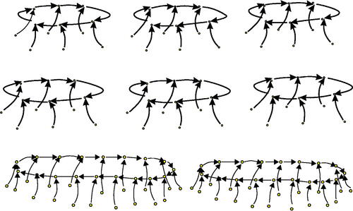
Example.
By Theorem 1, has 144 nodes. and it turns out that
(i.e., ), where the jellyfish can be ordered so that
have bell heads with cycle length 6, and J7 and J8 have bell heads with cycle length 18 (). By Theorem 3 (1), the nodes in
map to the eight Legendre curves with 18 preimages each. The 6 smaller jellyfish give the isogeny graph depicted in .
Fig. 2 2D rendering of the isogeny graph of each .
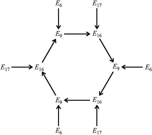
Fig. 3 swarm.
This defines the 3-to-1 covering These Legendre curves satisfy
We have For J7 and
we obtain the 9-to-1 covering
with
Therefore, we have
This example shows that individual jellyfish generally include many non-isomorphic curves, as the j-invariants (see (2.2)) for the smaller (resp. larger) jellyfish are and
(resp.
and
). We shall show that the number of different j-invariants, like counting types of spots on jellyfish, has taxonomic significance.
Thanks to the deeper insight offered by Corollary 4, we are able to revisit the baffling numbers and offer a nontrivial lower bound.
Theorem 5.
If , then for sufficiently large
we have
Remark.
Is this lower bound close to the truth? In view of examples such asit is tempting to speculate that this lower bound is not much smaller than an optimal bound which perhaps might be of the form
Proof of Theorem 5.
Corollary 4 guarantees that is at least as large as the number of distinct groups G for which
for some
For a group G, the proof of Theorem 6 establishes the existence of such a curve provided
and there is an
for which
We can construct many such groups. If and
then let
A classical theorem of Rück and Voloch [Citation15, Citation21] guarantees that one can take
For large q, this represents approximately one eighth of the integers in
Therefore, if
then for sufficiently large q we have
(2.4)
(2.4)
3 Jellyfish swarms and Gauss’ Class numbers
The swarms offer new descriptions of the class numbers studied by Gauss, Hurwitz and Kronecker (see [Citation5] for more on class numbers). To make this precise, recall that an integral binary quadratic form is a homogeneous degree 2 polynomial
The discriminantFootnote3 of f is If a > 0 and
then f(x, y) is called positive definite. Furthermore, f is primitive if
For negative discriminants D, the group
acts on
the set of positive definite binary quadratic forms of discriminant D. More precisely, for any
we have
Although there are infinitely many primitive binary quadratic forms with discriminant D, Gauss proved that their number of -orbits is finite, and this number is known as Gauss’ class number
Gauss’ class numbers lead to the more general Hurwitz-Kronecker class numbers. If , then the Hurwitz-Kronecker class number H(N) is the class number of positive definite integral binary quadratic forms of discriminant
where each class C is counted with multiplicity
If
where D is a negative fundamental discriminant (i.e., the discriminant of the ring of integers of an imaginary quadratic field), then H(N) is related to h(D) by (for example, see p. 273 of [Citation5])
Here w(D) is half the number of integral units in , and
denotes the sum of the sth powers of the positive divisors of n, and
is the quadratic Dirichlet character with conductor D.
Class numbers have a long and rich history. For example, class numbers play a central role in the study of quadratic forms. Indeed, if denotes the number of representations of an integer n as a sum of three squares, then Gauss proved that
Class numbers play even deeper roles in algebraic and analytic number theory, as they are the orders of ideal class groups of rings of integers and orders of imaginary quadratic fields. These groups themselves are the Galois groups of Hilbert class fields. For brevity, we simply say that the study of class numbers continues to drive cutting edge research today.
The jellyfish swarms offer a new interpretation of these class numbers. As the nodes are jellyfish spots, it is quite gratifying to discover that class numbers represent the number of types of spots that appear in a family of jellyfish. In this analogy, the j-invariants distinguish these types of spots. Namely, for integers s, let
be the number of distinct j-invariants of curves in the union of jellyfish with
the “Frobenius trace s family.” We have the following attractive description which follows from a well-known theorem of Schoof.
Theorem 6.
Suppose that is a finite field with
and
If
is a nonzero integer with
then we have
Example.
We revisit the example of , where
(resp. J7 and J8) are the smaller (resp. larger) jellyfish. We found earlier that the Frobenius trace -4 family is
One checks (using (2.2) that and
giving
We also found that the Frobenius trace 4 family is
As and
we also have
Therefore, since
, Theorem 6 gives
Proof of Theorem 6.
Let be an elliptic curve for which
and
We automatically have
because these groups can always be described as a direct product of at most 2 cyclic groups. Moreover, an application of the 2-descent lemma (for example, see Proposition 3.3 of [Citation1]) implies that there is an
for which
Conversely, every
is such an E thanks to Corollary 4. Therefore,
encodes the isomorphism classes of elliptic curves
with
with the additional property that
where
.
We consider the isomorphism classes of such curves with fixed nonzero trace of Frobenius s. If
satisfies
then either
or they are nontrivial twists of each other (see Chapter X of [Citation16]). In the latter case, the traces of Frobenius differ in sign.
Combining these facts, we have that is the number of isomorphism classes of elliptic curves
with
and trace of Frobenius s. The rich theory of complex multiplication for elliptic curves is the bridge which connects the counts of such classes with equivalence classes of binary quadratic forms. Indeed, a well-known deep theorem of Schoof (see Section 4 of [Citation18]) asserts that
equals the number of such isomorphism classes of elliptic curves. Invoking this theorem completes the proof. □
4 Analogies between Hypergeometric functions
Does the classical have more in common with its finite field analogues than the inductive rules
This is indeed the case. It turns out that the results offered above are a byproduct of remarkable analogies between complex hypergeometric functions and their finite field analogues. Let us explain.
Hypergeometric functions and
The theory underlying (see Chapter 1 of [Citation3]) is a story involving special integrals and their relationship with Gauss’ hypergeometric functions. To make this precise, for
we let
(4.1)
(4.1) where the polynomial in the square-root in the denominator of the integrand is tantalizinglyFootnote4 close to the cubic in the Legendre curve
It is straightforward to check that which in turn implies that
satisfies
(4.2)
(4.2)
Gauss discovered a beautiful formula for in terms of hypergeometric functions. For
and
these functions are defined by
(4.3)
(4.3) where
is the Pochhammer symbol defined by
Gauss’ theory of elliptic integrals [Citation9, p. 182] gives(4.4)
(4.4) which, by letting
and
also gives
(4.5)
(4.5)
Equating these expressions, we find that leads to the identity
which relates
with
This identity is a special case (i.e.,
and
) of the far more general quadratic transformation formula (see [Citation2, (3.1.11)])
(4.6)
(4.6)
Hypergeometric functions and
In view of the previous discussion, we seek a finite field analog of
To this end, one can replace the integral over by a sum over
and replace the square-root with the quadratic character
and we can naively declare the finite field analogue to be the sum
(4.7)
(4.7)
We hope that such sums are values of hypergeometric-type functions.
In his important 1984 Ph.D. thesis [Citation7], Greene defined the finite field hypergeometric functions that do the trick (see [Citation13, Citation14] for applications). For multiplicative charactersFootnote5 and
of
he defined
where the sum is over the multiplicative characters of
and
is the normalized Jacobi sum
This definition was meant to resemble (4.3), and is based on analogies between Gauss sums and the complex Γ-function, which interpolates factorials, and the classical Gauss sum expression for Jacobi sums (when is nontrivial)
which in turn emulates binomial coefficients.
These functions take an attractive form when n = 2 (see p. 82 of [Citation8]). If A, B, and C are characters of and
then
In particular, if and
is trivial, then a change of variables gives
(4.8)
(4.8)
In analogy with Gauss’ integral formulas, which give periods of elliptic curves, Greene’s functions compute traces of Frobenius over Indeed, if
and
then (4.8) gives
(4.9)
(4.9)
In terms of the desired analogy, if then (4.7) and (4.8) gives the counterpart of (4.4)
To complete the analogy, we require a quadratic transformation law which plays the role of (4.6). We conclude by stating this recent theorem of Evans and Greene (see Theorem 2 of [Citation6]), which precisely offers the desired analogous transformation.
Theorem 7.
[Theorem 2 of [Citation6]] Suppose that A, and
are all nontrivial characters of
If
then
5 Epilogue
We hope that the reader agrees that the story presented here is a beautiful amalgamation of facts about elliptic curves over and over finite fields. It is quite marvelous to find that the hypergeometric functions of Gauss (in the case of
) and of Greene (in the case of
) underlie different features in the theory of elliptic curves that are captured by sequences of arithmetic and geometric means. We hope that this story encourages readers to learn more about the theory of Gauss’ class numbers, elliptic curves, and hypergeometry. We highly recommend D. Cox’s book “Primes of the form
” [Citation5] and “Pi and the AGM” [Citation3] by P. Borwein and J. Borwein.
We aim to entice readers with the following tantalizing problems.
Problems.
What can one prove about the sizes of the jellyfish in
Determine an “optimal” function D(q) for which
It would be very interesting to define variants of
To conclude, we must confess that the jellyfish are merely alluring examples of creatures that inhabit the magnificent kingdom formed out of elliptic curves over finite fields. The beautiful
sequences innocently offer glimpses of the fascinating theory of isogenies for elliptic curves over finite fields, which form networks, dubbed isogeny volcanoes. The jellyfish are examples that arise from “2-volcanoes of height 1.” Isogeny volcanoes play important roles in computational number theory and cryptography. They are often employed as a means of accelerating number theoretic algorithms. They have even been used to quickly compute values of Euler’s partition function [Citation4]. This important theory has its origins in David Kohel’s Citation1996 Ph.D. thesis [Citation11]. We invite interested readers to read the delightful expository article [Citation19] by Sutherland.
Acknowledgment
The authors thank the referees, Jennifer Balakrishnan, Hasan Saad, and Drew Sutherland for comments and suggestions that improved this article. The second author thanks the Thomas Jefferson Fund and the NSF (DMS-2002265 and DMS-2055118) for their generous support, as well as the Kavli Institute grant NSF PHY-1748958. The third author is grateful for the support of a Fulbright Nehru Postdoctoral Fellowship.
Additional information
Funding
Notes on contributors
Michael J. Griffin
MICHAEL J. GRIFFIN received the Ph.D. degree in Mathematics from Emory University in 2015. He is an Assistant Professor of Mathematics at Brigham University in Provo, Utah, USA. His research interests are in number theory.
Ken Ono
KEN ONO received the Ph.D. degree in Mathematics from UCLA in 1993. He is the Thomas Jefferson Professor of Mathematics at the University of Virginia, Charlottesville, Virginia, USA. His research interests are in number theory.
Neelam Saikia
NEELAM SAIKIA received the Ph.D. degree in Mathematics from the Indian Institute of Technology in Delhi, India in 2016. She is an Assistant Professor of Mathematics at the Indian Institute of Technology Bhubaneswar in Bhubaneswar, Odisha, India. Her research interests are in number theory.
Wei-Lun Tsai
WEI-LUN TSAI received the Ph.D. degree in Mathematics from the Texas A&M University in 2020. He is a Research Postdoctoral Fellow at the University of Virginia, Charlottesville, Virginia, USA. His research interests are in number theory.
Notes
1 There are no loops (i.e., ) as nodes of the form (a, a) are not allowed.
2 The proof of Theorem 3 shows that the swarms are graphs of 2-isogenies. We point interested readers to Sutherland’s expository article [Citation19] for more on the theory of isogeny graphs.
3 Discriminants always satisfy
4 These models are actually –1 quadratic twists of each other.
5 For multiplicative characters χ, we adopt the convention that
References
- Ahlgren, S., Ono, K. (2000). Modularity of a certain Calabi-Yau threefold. Montash. Math. 129(3): 177–190.
- Andrews, G., Askey, R., Roy, R. (2001). Special Functions. Cambridge: Cambridge Univ. Press.
- Borwein, J., Borwein, P. (1998). Pi and the AGM. New York: Wiley.
- Bruinier, J. H., Ono, K., Sutherland, A. V. (2016). Class polynomials for nonholomorphic modular functions. J. Number Theory 161: 204–229. DOI: 10.1016/j.jnt.2015.07.002.
- Cox, D. A. (2013). Primes of the Form x2+ny2. New York: Wiley.
- Evans, R., Greene, J. (2017). A quadratic hypergeometric 2F1 transformation over finite fields. Proc. Amer. Math. Soc. 145: 1071–1076.
- Greene, J. (1984). Character sum analogues for hypergeometric and generalized hypergeometric functions over finite fields. Ph.D. Dissertation. Univ. of Minnesota, Minneapolis, USA.
- Greene, J. (1987). Hypergeometric functions over finite fields. Trans. Amer. Math. Soc. 301: 77–101. DOI: 10.1090/S0002-9947-1987-0879564-8.
- Husemöller, D. (2004). Elliptic Curves. New York: Springer.
- Koblitz, N. (1993). Introduction to Elliptic Curves and Modular Forms, 2nd ed. New York: Springer.
- Kohel, D. (1996). Endomorphism rings of elliptic curves over finite fields. Ph.D. Dissertation. Univ. of California, Berkeley, USA.
- Mazur, B. (1991). Number theory as gadfly. Amer. Math. Monthly. 98(7): 593–610. DOI: 10.1080/00029890.1991.11995762.
- Ono, K. (1998). Values of Gaussian hypergeometric series. Trans. Amer. Math. Soc. 350(3): 1205–1223.
- Ono, K. (2004). The Web of Modularity. Providence: Amer. Math. Soc.
- Rück, H.-G. (1987). A note on elliptic curves over finite fields. Math. Comp. 49: 301–304.
- Silverman, J. (2009). The Arithmetic of Elliptic Curves, 2nd ed. New York: Springer.
- Silverman, J. (1993). Taxicabs and sums of two cubes. Amer. Math. Monthly. 100(4): 331–340.
- Schoof, R. (1987). Nonsingular plane cubic curves over finite fields. J. Comb. Theory Ser. A. 46(2): 183–211.
- Sutherland, A. V. (2013). Isogeny volcanoes. ANTS X- Proc. Algorithmic Number Theory Symposium. Berkeley: Mathematical Sciences Publishers, pp. 507–530.
- Taylor, R., Wiles, A. (1995). Ring theoretic properties of certain Hecke algebras. Ann. Math. 141: 553–572. DOI: 10.2307/2118560.
- Voloch, J. F. (1988). A note on elliptic curves over finite fields. Bull. Soc. Math. France. 116: 455–458. DOI: 10.24033/bsmf.2107.
- Washington, L. C. (2008). Elliptic Curves, Number Theory, and Cryptography, Boca Raton: Chapman & Hall.
- Wiles, A. (1995). Modular elliptic curves and Fermat’s Last theorem. Ann. Math. 141: 443–551. DOI: 10.2307/2118559.