Bayesian Inference for Kendall’s Rank Correlation Coefficient

ABSTRACT

This article outlines a Bayesian methodology to estimate and test the Kendall rank correlation coefficient τ. The nonparametric nature of rank data implies the absence of a generative model and the lack of an explicit likelihood function. These challenges can be overcome by modeling test statistics rather than data. We also introduce a method for obtaining a default prior distribution. The combined result is an inferential methodology that yields a posterior distribution for Kendall’s τ.

KEYWORDS:

• Bayes factor
• Kendall’s tau
• Nonparametric inference

1. Introduction

One of the most widely used nonparametric tests of dependence between two variables is the rank correlation known as Kendall’s τ (Kendall 1938). Compared to Pearson’s ρ, Kendall’s τ is robust to outliers and violations of normality (Kendall and Gibbons 1990). Moreover, Kendall’s τ expresses dependence in terms of monotonicity instead of linearity and is therefore invariant under rank-preserving transformations of the measurement scale (Kruskal 1958; Wasserman 2006). As expressed by Harold Jeffreys (1961, p. 231): “[...] it seems to me that the chief merit of the method of ranks is that it eliminates departure from linearity, and with it a large part of the uncertainty arising from the fact that we do not know any form of the law connecting X and Y.” Here, we apply the Bayesian inferential paradigm to Kendall’s τ. Specifically, we define a default prior distribution on Kendall’s τ, obtain the associated posterior distribution, and use the Savage–Dickey density ratio to obtain a Bayes factor hypothesis test (Jeffreys 1961; Dickey and Lientz 1970; Kass and Raftery 1995).

1.1. Kendall’s τ

Let X = (x₁, …, x_n) and Y = (y₁, …, y_n) be two data vectors each containing measurements of the same n units. For example, consider the association between French and math grades in a class of n = 3 children: Tina, Bob, and Jim; let X = (8, 7, 5) be their grades for a French exam and Y = (9, 6, 7) be their grades for a math exam. For 1 ⩽ i < j ⩽ n, each pair (i, j) is defined to be a pair of differences (x_i − x_j) and (y_i − y_j). A pair is considered to be concordant if (x_i − x_j) and (y_i − y_j) share the same sign, and discordant when they do not. In our data example, Tina has higher grades on both exams than Bob, which means that Tina and Bob are a concordant pair. Conversely, Bob has a higher score for French, but a lower score for math than Jim, which means Bob and Jim are a discordant pair. The observed value of Kendall’s τ, denoted τ_obs, is defined as the difference between the number of concordant and discordant pairs, expressed as proportion of the total number of pairs (1) $$\begin{array}{c}\hfill {\tau }_{\mathrm{obs}}=\frac{{\sum }_{1\le i<j\le n}^{n}Q((x_i,y_i),(x_j,y_j))}{n(n-1)/2},\end{array}$$(1) where the denominator is the total number of pairs and Q is the concordance indicator function (2) $$\begin{array}{c}\hfill Q\left((x_i,y_i)(x_j,y_j)\right)=\left\{\begin{array}{cc}\hfill -1& \hfill \text{if}(x_i-x_j)(y_i-y_j)<0\\ \hfill +1& \hfill \text{if}(x_i-x_j)(y_i-y_j)>0\end{array}\right..\end{array}$$(2)

Table 1 illustrates the calculation for our small data example. Applying Equation (1(1) $$\begin{array}{c}\hfill {\tau }_{\mathrm{obs}}=\frac{{\sum }_{1\le i<j\le n}^{n}Q((x_i,y_i),(x_j,y_j))}{n(n-1)/2},\end{array}$$(1) ) gives τ_obs = 1/3, an indication of a positive correlation between French and math grades.

Table 1. The pairs (i, j) for 1 ⩽ i < j ⩽ n and the concordance indicator function Q for the data example where X = (8, 7, 5) and Y = (9, 6, 7).

i	j	(xi − xj)	(yi − yj)	Q
1	2	8 − 7	9 − 6	1
1	3	8 − 5	9 − 7	1
2	3	7 − 5	6 − 7	−1

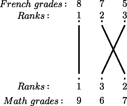
When τ_obs = 1, all pairs of observations are concordant, and when τ_obs = −1, all pairs are discordant. Kruskal (1958) provided the following interpretation of Kendall’s τ: in the case of n = 2, suppose we bet that y₁ < y₂ whenever x₁ < x₂, and that y₁ > y₂ whenever x₁ > x₂; winning $1 after a correct prediction and losing $1 after an incorrect prediction, the expected outcome of the bet equals τ. Furthermore, Griffin (1958) had illustrated that when the ordered rank-converted values of X are placed above the rank-converted values of Y and lines are drawn between the same numbers, Kendall’s τ_obs is given by the formula: $1-\frac{4z}{n(n-1)}$, where Z is the number of line intersections; see Figure 1 for an illustration of this method using our example data of French and math grades. These tools make for a straightforward and intuitive calculation and interpretation of Kendall’s τ.

Figure 1. A visual interpretation of Kendall’s τ_obs through the formula: $1-\frac{4z}{n(n-1)}$, where z is the number of intersections of the lines. In this case, n = 3, z = 1, and τ_obs = 1/3.

Despite these appealing properties and the overall popularity of Kendall’s τ, a default Bayesian inferential paradigm is still lacking because the application of Bayesian inference to nonparametric data analysis is not trivial. The main challenge in obtaining posterior distributions and Bayes factors for nonparametric tests is that there is no generative model and no explicit likelihood function. In addition, Bayesian model specification requires the specification of a prior distribution, and this is especially important for Bayes factor hypothesis testing; however, for nonparametric tests it can be challenging to define a sensible default prior. Though recent developments have been made in two-sample nonparametric Bayesian hypothesis testing with Dirichlet process priors (Borgwardt and Ghahramani 2009; Labadi, Masuadi, and Zarepour 2014) and Pòlya tree priors (Chen and Hanson 2014; Holmes et al. 2015), this article will outline a different approach, one that permits an intuitive and direct interpretation.

1.2. Modeling Test Statistics

To compute Bayes factors^{Table 1Figure 1} for Kendall’s τ, we start with the approach pioneered by Johnson (2005) and Yuan and Johnson (2008). These authors established bounds for Bayes factors based on the sampling distribution of the standardized value of τ, denoted by T*, which will be formally defined in Section 2.1. Using the Pitman translation alternative, where a noncentrality parameter is used to distinguish between the null and alternative hypotheses (Randles and Wolfe 1979), Johnson and colleagues specified the following hypotheses (3) $$\begin{array}{c}\hfill {\mathcal{H}}_0:\theta ={\theta }_0,\end{array}$$(3) (4) $$\begin{array}{c}\hfill {\mathcal{H}}_1:\theta ={\theta }_0+\frac{\Delta }{\sqrt{n}},\end{array}$$(4) where θ is the true underlying value of Kendall’s τ, θ₀ is the value of Kendall’s τ under the null hypothesis, and Δ serves as the noncentrality parameter that can be assigned a prior distribution. The limiting distribution of T* under both hypotheses is normal (Hotelling and Pabs 1936; Noether 1955; Chernoff and Savage 1958), with likelihoods $$\begin{array}{ccc}& & {\mathcal{H}}_0:T^{*}\sim N(0,1)\hfill \\ & & {\mathcal{H}}_1:T^{*}\sim N\left(\frac{3\Delta }{2},1\right).\hfill \end{array}$$The prior on Δ is specified by Yuan and Johnson as $$\Delta \sim N(0,{\kappa }^2),$$where κ is used to specify the expectation about the size of the departure from the null-value of Δ. This leads to the following Bayes factor (5) $$\begin{array}{c}\hfill {\text{BF}}_{01}=\sqrt{1+\frac{9}{4}{\kappa }^2}exp\left(-\frac{{\kappa }^2{T}^{*2}}{2{\kappa }^2+\frac{8}{9}}\right).\end{array}$$(5)

Next, Yuan and Johnson calculated an upper bound on ${\text{BF}}_{10}$ (i.e., a lower bound on ${\text{BF}}_{01}$) by maximizing over the parameter κ.

1.3. Challenges

Although innovative and compelling, the approach advocated by Yuan and Johnson (2008) does have a number of non-Bayesian elements, most notably the data-dependent maximization over the parameter κ that results in a data-dependent prior distribution. Moreover, the definition of ${\mathcal{H}}_1$ depends on n: as n → ∞, ${\mathcal{H}}_1$ and ${\mathcal{H}}_0$ become indistinguishable and lead to an inconsistent inferential framework.

Our approach, motivated by the earlier work by Johnson and colleagues, sought to eliminate κ not by maximization but by a method we call “parametric yoking” (i.e., matching with a prior distribution for a parametric alternative). In addition, we redefined ${\mathcal{H}}_1$ such that its definition does not depend on sample size. As such, Δ becomes synonymous with the true underlying value of Kendall’s τ when θ₀ = 0.

2. Methods

2.1. Defining T*

As mentioned earlier, Yuan and Johnson (2008) used the standardized version of τ_obs, denoted T* (Kendall 1938), which is defined as follows (6) $$\begin{array}{c}\hfill T^{*}=\frac{{\sum }_{1\le i<j\le n}^{n}Q((x_i,y_i),(x_j,y_j))}{\sqrt{n(n-1)(2n+5)/18}}.\end{array}$$(6)

Here the numerator contains the concordance indicator function Q. Thus, T* is not necessarily situated between the traditional bounds [−1,1] for a correlation; instead, T* has a maximum of $\sqrt{\frac{9n(n-1)}{4n+10}}$ and a minimum of $-\sqrt{\frac{9n(n-1)}{4n+10}}$. This definition of T* enables the asymptotic normal approximation to the sampling distribution of the test statistic (Kendall and Gibbons 1990).

2.2. Prior Distribution through Parametric Yoking

To derive a Bayes factor for τ, we first determine a default prior for τ through what we term parametric yoking. In this procedure, a default prior distribution is constructed by comparison to a parametric alternative. In this case, a convenient parametric alternative is given by Pearson’s correlation for bivariate normal data. Ly, Verhagen, and Wagenmakers (2016) used a symmetric beta prior distribution (α = β) on the domain [−1,1], that is, (7) $$\begin{array}{c}\hfill p\left(\rho \right)=\frac{2^{1-2\alpha }}{\mathcal{B}(\alpha ,\alpha )}\times {(1-{\rho }^2)}^{(\alpha -1)},\rho \in (-1,1),\end{array}$$(7) where $\mathcal{B}$ is the beta function. For bivariate normal data, Kendall’s τ is related to Pearson’s ρ by Greiner’s relation (Greiner 1909; Kruskal 1958) (8) $$\begin{array}{c}\hfill \tau =\frac{2}{\pi }\arcsin \left(\rho \right).\end{array}$$(8)

We can use this relationship to transform the beta prior in (7(7) $$\begin{array}{c}\hfill p\left(\rho \right)=\frac{2^{1-2\alpha }}{\mathcal{B}(\alpha ,\alpha )}\times {(1-{\rho }^2)}^{(\alpha -1)},\rho \in (-1,1),\end{array}$$(7) ) on ρ to a prior on τ given by (9) $$\begin{array}{c}\hfill p\left(\tau \right)=\pi \frac{2^{-2\alpha }}{\mathcal{B}(\alpha ,\alpha )}\times cos{\left(\frac{\pi \tau }{2}\right)}^{(2\alpha -1)},\tau \in (-1,1).\end{array}$$(9) In the absence of strong prior beliefs, Jeffreys (1961) proposed a uniform distribution on ρ, that is, a stretched beta with α = β = 1. This induces a nonuniform distribution on τ, that is, (10) $$\begin{array}{c}\hfill p\left(\tau \right)=\frac{\pi }{4}cos\left(\frac{\pi \tau }{2}\right).\end{array}$$(10) Values of α ≠ 1 can be specified to induce different prior distributions on τ. In general, values of α > 1 increase the prior mass near τ = 0, whereas values of α < 1 decrease the prior mass near τ = 0. When the focus is on parameter estimation instead of hypothesis testing, we may follow Jeffreys (1961) and use a stretched beta prior on ρ with $\alpha =\beta =1/2$. As is easily confirmed by entering these values in (9(9) $$\begin{array}{c}\hfill p\left(\tau \right)=\pi \frac{2^{-2\alpha }}{\mathcal{B}(\alpha ,\alpha )}\times cos{\left(\frac{\pi \tau }{2}\right)}^{(2\alpha -1)},\tau \in (-1,1).\end{array}$$(9) ), this choice induces a uniform prior distribution for Kendall’s τ. (Additional examples and figures of the stretched beta prior, including cases where α ≠ β, are available online at https://osf.io/b9qhj/.) The parametric yoking framework can be extended to other prior distributions that exist for Pearson’s ρ (e.g., the inverse Wishart distribution; Gelman et al. 2003; Berger and Sun 2008), by transforming ρ with the inverse of the expression given in (8(8) $$\begin{array}{c}\hfill \tau =\frac{2}{\pi }\arcsin \left(\rho \right).\end{array}$$(8) ): $$\rho =sin\left(\frac{\pi \tau }{2}\right).$$

2.3. Posterior Distribution and Bayes Factor

Removing $\sqrt{n}$ from the specification of ${\mathcal{H}}_1$ by substituting $\Delta \sqrt{n}$ for Δ, the likelihood function under ${\mathcal{H}}_1$ equals a normal density with mean $\mu =\frac{3}{2}\Delta \sqrt{n}$ and standard deviation σ = 1: (11) $$\begin{array}{c}\hfill p\left(T^{*}\right|{\theta }_0+\Delta )=\frac{1}{\sqrt{2\pi }}exp\left(-\frac{{(T^{*}-(3/2)\Delta \sqrt{n})}^2}{2}\right).\end{array}$$(11) Combining this normal likelihood function with the prior from (9(9) $$\begin{array}{c}\hfill p\left(\tau \right)=\pi \frac{2^{-2\alpha }}{\mathcal{B}(\alpha ,\alpha )}\times cos{\left(\frac{\pi \tau }{2}\right)}^{(2\alpha -1)},\tau \in (-1,1).\end{array}$$(9) ) yields the posterior distribution for Kendall’s τ. Next, Bayes factors can be computed as the ratio of the prior and posterior ordinate at the point under test (i.e., the Savage-Dickey density ratio, Dickey and Lientz 1970; Wagenmakers et al. 2010). In the case of testing independence, the point under test is τ = 0, leading to the following ratio: ${\text{BF}}_{01}=\frac{p(\tau =0\mid y)}{p(\tau =0)}$, which is analogous to (12) $$\begin{array}{c}\hfill {\text{BF}}_{01}=\frac{p\left(T^{*}\right|{\theta }_0)}{\int p\left(T^{*}\right|{\theta }_0+\Delta )p\left(\Delta \right)d\Delta },\end{array}$$(12) and in the case of Kendall’s τ translates to (13) $$\begin{array}{c}\hfill {\text{BF}}_{01}=\frac{exp(-\frac{T^{*2}}{2})}{{\int }_{-1}^{1}exp\left(-\frac{{(T^{*}-(3/2)\tau \sqrt{n})}^2}{2}\right)\left(\pi \frac{2^{-2\alpha }}{\mathcal{B}(\alpha ,\alpha )}\times cos{\left(\frac{\pi \tau }{2}\right)}^{(2\alpha -1)}\right)d\tau }.\end{array}$$(13)

2.4. Verifying the Asymptotic Normality of T*

Our method relies on the asymptotic normality of T*, a property established mathematically by Hoeffding (1948). For practical purposes, however, it is insightful to assess the extent to which this distributional assumption is appropriate for realistic sample sizes. By considering all possible permutations of the data, deriving the exact cumulative density of T*, and comparing the densities to those of a standard normal distribution, Ferguson, Genest, and Hallin (2000) concluded that the normal approximation holds under ${\mathcal{H}}_0$ when n ⩾ 10. But what if ${\mathcal{H}}_0$ is false?

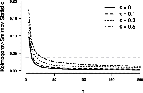
Here, we report a simulation study designed to assess the quality of the normal approximation to the sampling distribution of T* when ${\mathcal{H}}_1$ is true. With the use of copulas, 100,000 synthetic datasets were created for each of several combinations of Kendall’s τ and sample size n. (For more information on copulas see Nelsen (2006), Genest and Favre (2007), and Colonius (2016).) For each simulated dataset, the Kolmogorov–Smirnov statistic was used to quantify the fit of the normal approximation to the sampling distribution of T*. (R code, plots, and further details are available online at https://osf.io/b9qhj/.) Figure 2 shows the Kolmogorov–Smirnov statistic as a function of n, for various values of τ when datasets were generated from a bivariate normal distribution (i.e., the normal copula). Similar results were obtained using Frank, Clayton, and Gumbel copulas. As is the case under ${\mathcal{H}}_0$ (e.g., Kendall and Gibbons 1990; Ferguson, Genest, and Hallin 2000), the quality of the normal approximation increases exponentially with n. Furthermore, larger values of τ necessitate larger values of n to achieve the same quality of approximation.

Figure 2. Quality of the normal approximation to the sampling distribution of T*, as assessed by the Kolmogorov–Smirnov statistic. As n grows, the quality of the normal approximation increases exponentially. Larger values of τ necessitate larger values of n to achieve the same quality of approximation. The gray horizontal line corresponds to a Kolmogorov–Smirnov statistic of 0.038 (obtained when τ = 0 and n = 10), for which Ferguson, Genest, and Hallin (2000, p. 589) deemed the quality of the normal approximation to be “sufficiently precise for practical purposes.”

The means of the normal distributions fit to the sampling distribution of T* are situated at the point $\frac{3}{2}\Delta \sqrt{n}$. The datasets from this simulation can also be used to examine the variance of the normal approximation. Under ${\mathcal{H}}_0$ (i.e., τ = 0), the variance of these normal distributions equals 1. As the population correlation grows (i.e., |τ| → 1), the number of permissible rank permutations decreases and so does the variance of T*. The upper bound of the sampling variance of T* is a function of the population value for τ (Kendall and Gibbons 1990): (14) $$\begin{array}{c}\hfill {\sigma }_{T^{*}}^2\le \frac{2.5n(1-{\tau }^2)}{2n+5}.\end{array}$$(14) As shown in the online appendix, our simulation results provide specific values for the variance, which respect this upper bound. This result has ramifications for the Bayes factor. As the test statistic moves away from 0, the variance falls below 1, and the posterior distribution will be more peaked on the value of the test statistic than when the variance is assumed to equal 1. This results in increased evidence in favor of ${\mathcal{H}}_1$, so that our proposed procedure is somewhat conservative. However, for n ⩾ 20, the changes in variance will only surface in cases where there already exists substantial evidence for ${\mathcal{H}}_1$ (i.e., ${\text{BF}}_{10}\ge 10$).

3. Results

3.1. Bayes Factor Behavior

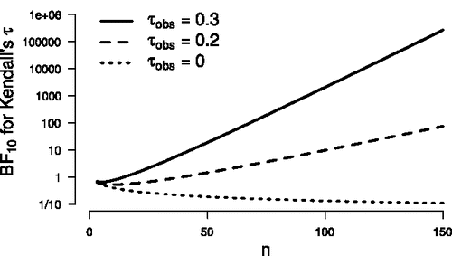
Now that we have determined a default prior for τ and combined it with the specified Gaussian likelihood function, computation of the posterior distribution and the Bayes factor becomes feasible. For an uninformative prior on τ (i.e., α = β = 1), Figure 3 illustrates ${\text{BF}}_{10}$ as a function of n, for three values of τ_obs. The lines for τ_obs = 0.2 and τ_obs = 0.3 show that ${\text{BF}}_{10}$ for a true ${\mathcal{H}}_1$ increases exponentially with n, as is generally the case. For τ_obs = 0, the Bayes factor decreases as n increases.

Figure 3. Relation between ${\text{BF}}_{10}$ and sample size (3 ⩽ n ⩽ 150) for three values of Kendall’s τ.

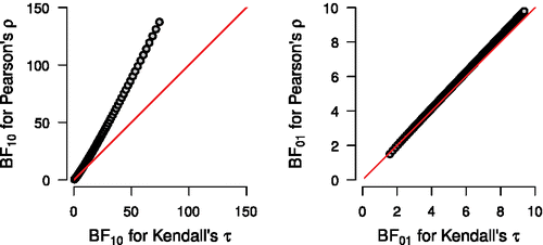
3.2. Comparison to Pearson’s ρ

To put the result in perspective, the Bayes factors for Kendall’s tau (i.e., ${\text{BF}}_{10}^{\tau }$) can be compared to those for Pearson’s ρ (i.e., ${\text{BF}}_{10}^{\rho }$). The Bayes factors for Pearson’s ρ are based on Jeffreys (1961, see also Ly, Verhagen, and Wagenmakers 2016), who used the uniform prior on ρ. Figure 4 shows that the relationship between ${\text{BF}}_{10}^{\tau }$ and ${\text{BF}}_{10}^{\rho }$ for normal data is approximately linear as a function of sample size. In addition, and as one would expect due to the loss of information when continuous values are converted to coarser ranks, ${\text{BF}}_{10}^{\tau }<{\text{BF}}_{10}^{\rho }$ in the case of evidence in favor of ${\mathcal{H}}_1$ (left panel of Figure 4). When evidence is in favor of ${\mathcal{H}}_0$, that is, τ = 0, ${\text{BF}}_{10}^{\tau }\text{and}{\text{BF}}_{10}^{\rho }$ perform similarly (right panel of Figure 4).

Figure 4. Relation between the Bayes factors for Pearsons ρ and Kendall’s τ = 0.2 (left) and Kendall’s τ = 0 (right) as a function of sample size (i.e., 3 ⩽ n ⩽ 150). The data are normally distributed. Note that the left panel shows ${\text{BF}}_{10}$ and the right panel shows ${\text{BF}}_{01}$. The diagonal line indicates equivalence.

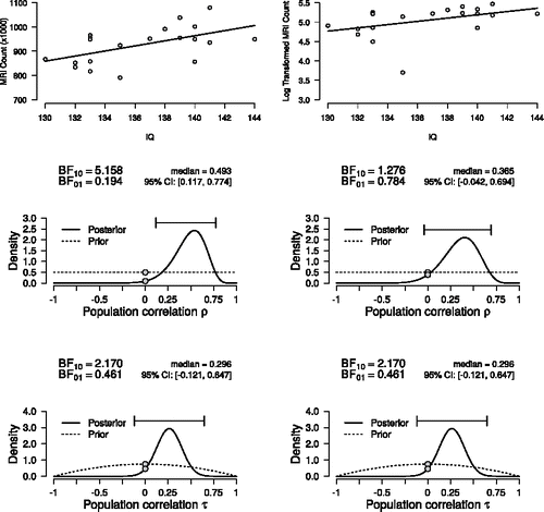
3.3. Real Data Example

Willerman et al. (1991) set out to uncover the relation between brain size and IQ. Across 20 participants, the authors observed a Pearson’s correlation coefficient of r = 0.51 between IQ and brain size, measured in MRI count of gray matter pixels. The data are presented in the top left panel of Figure 5. Bayes factor hypothesis testing of Pearson’s ρ yields ${\text{BF}}_{10}^{\rho }=5.16$, which is illustrated in the middle left panel. This means the data are 5.16 times as likely to occur under ${\mathcal{H}}_1$ than under ${\mathcal{H}}_0$. When applying a log-transformation on the MRI counts (after subtracting the minimum value minus 1), however, the linear relation between IQ and brain size is less strong. The top right panel of Figure 5 presents the effect of this monotonic transformation on the data. The middle right panel illustrates how the transformation decreases ${\text{BF}}_{10}^{\rho }$ to 1.28. The bottom left panel presents our Bayesian analysis on Kendall’s τ, which yields a ${\text{BF}}_{10}^{\tau }$ of 2.17. Furthermore, the bottom right panel shows the same analysis on the transformed data, illustrating the invariance of Kendall’s τ against monotonic transformations: the inference remains unchanged, which highlights one of Kendall’s τ most appealing features.

Figure 5. Bayesian inference for Kendall’s τ illustrated with data on IQ and brain size (Willerman et al. 1991). The left column presents the relation between brain size and IQ, analyzed using Pearson’s ρ (middle panel) and Kendall’s τ (bottom panel). The right column presents the results after a log transformation of brain size. Note that the transformation affects inference for Pearson’s ρ, but does not affect inference for Kendall’s τ.

4. Concluding Comments

This manuscript outlined a nonparametric Bayesian framework for inference about Kendall’s tau. The framework is based on modeling test statistics and assigning a prior by means of a parametric yoking procedure. The framework produces a posterior distribution for Kendall’s tau, and—via the Savage-Dickey density ratio test—also yields a Bayes factor that quantifies the evidence for the absence of a correlation.

Our general procedure (i.e., modeling test statistics and assigning a prior through parametric yoking) is relatively general and may be used to facilitate Bayesian inference for other nonparametric tests as well. For instance, Serfling (1980) offered a range of test statistics with asymptotic normality to which our framework may be expanded, whereas Johnson (2005) had explored the modeling of test statistics that have non-Gaussian limiting distributions.

Supplementary Materials

An online appendix, with more information on the different prior options, as well as the simulation study to assess the normality of Kendall's τ, is available online at https://osf.io/b9qhj/. This repository also contains R-code for Bayesian inference on Kendall's τ, as well as for the simulation study.

Additional information

Funding

The authors acknowledge support from the European Science Foundation (ERC grant 283876) and the Netherlands Organization for Scientific Research.

References

- Berger, J. O., and Sun, D. (2008), “Objective Priors for the Bivariate Normal Model,” The Annals of Statistics, 36, 963–982.
- Borgwardt, K. M., and Ghahramani, Z. (2009), “Bayesian Two-Sample Tests,” arXiv preprint arXiv:0906.4032.
- Chen, Y., and Hanson, T. E. (2014), “Bayesian Nonparametric k-Sample Tests for Censored and Uncensored Data,” Computational Statistics & Data Analysis, 71, 335–346.
- Chernoff, H., and Savage, R. (1958), “Asymptotic Normality and Efficiency of Certain Nonparametric Test Statistics,” The Annals of Statistics, 29, 972–994.
- Colonius, H. (2016), “An Invitation to Coupling and Copulas: With Applications to Multisensory Modeling,” Journal ofMathematical Psychology, 74, 2–10.
- Dickey, J. M., and Lientz, B. P. (1970), “The Weighted Likelihood Ratio, Sharp Hypotheses about Chances, the Order of a Markov Chain,” The Annals of Mathematical Statistics, 41, 214–226.
- Ferguson, T. S., Genest, C., and Hallin, M. (2000), “Kendall’s Tau for Serial Dependence,” Canadian Journal of Statistics, 28, 587–604.
- Gelman, A., Carlin, J., Stern, H., Dunson, D., Vehtari, A., and Rubin, D. (2003), Bayesian Data Analysis (2nd ed.), London: Chapman & Hall/CRC.
- Genest, C., and Favre, A.-C. (2007), “Everything You Always Wanted to Know About Copula Modeling but Were Afraid to Ask,” Journal of Hydrologic Engineering, 12, 347–368.
- Greiner, R. (1909), “Über das Fehlersystem der Kollektivmasslehre,” Zeitschift für Mathematik undPhysik, 57, 121–158.
- Griffin, H. (1958), “Graphic Computation of Tau as a Coefficient of Disarray,” Journal of the American Statistical Association, 53, 441–447.
- Hoeffding, W. (1948), “A Class of Statistics with Asymptotically Normal Distribution,” Annals of Mathematical Statistics, 19, 293–325.
- Holmes, C. C., Caron, F., Griffin, J. E., and Stephens, D. A. (2015), “Two-Sample Bayesian Nonparametric Hypothesis Testing,” Bayesian Analysis, 10, 297–320.
- Hotelling, H., and Pabs, M. (1936), “Rank Correlation and Tests of Significance Involving no Assumption of Normality,” Annals of Mathematical Statistics, 7, 29–43.
- Jeffreys, H. (1961), Theory of Probability (3rd ed.), Oxford, UK: Oxford University Press.
- Johnson, V. E. (2005), “Bayes Factors Based on Test Statistics,” Journal of the Royal Statistical Society, Series B, 67, 689–701.
- Kass, R. E., and Raftery, A. E. (1995), “Bayes Factors,” Journal of the American Statistical Association, 90, 773–795.
- Kendall, M. (1938), “A new Measure of Rank Correlation,” Biometrika, 30, 81–93.
- Kendall, M., and Gibbons, J. D. (1990), Rank Correlation Methods, New York: Oxford University Press.
- Kruskal, W. (1958), “Ordinal Measures of Association,” Journal of the American Statistical Association, 53, 814–861.
- Labadi, L. A., Masuadi, E., and Zarepour, M. (2014), “Two-Sample Bayesian Nonparametric Goodness-of-Fit Test,” arXiv preprintarXiv:1411.3427.
- Ly, A., Verhagen, A. J., and Wagenmakers, E.-J. (2016), “Harold Jeffreys’s Default Bayes Factor Hypothesis Tests: Explanation, Extension, and Application in Psychology,” Journal of Mathematical Psychology, 72, 19–32.
- Nelsen, R. (2006), An Introduction to Copulas (2nd ed.), New York: Springer-Verlag.
- Noether, G. E. (1955), “On a Theorem of Pitman,” Annals of Mathematical Statistics, 26, 64–68.
- Randles, R. H., and Wolfe, D. A. (1979), Introduction to the Theory of Nonparametric Statistics (Springer Texts in Statistics), New York: Wiley.
- Serfling, R. J. (1980), Approximation Theorems of Mathematical Statistics, New York: Wiley.
- Wagenmakers, E.-J., Lodewyckx, T., Kuriyal, H., and Grasman, R. (2010), “Bayesian Hypothesis Testing for Psychologists: A Tutorial on the Savage–Dickey Method,” Cognitive Psychology, 60, 158–189.
- Wasserman, L. (2006), All of Nonparametric Statistics (Springer Texts in Statistics), New York: Springer Science and Business Media.
- Willerman, L., Schultz, R., Rutledge, J. N., and Bigler, E. D. (1991), “In Vivo Brain Size and Intelligence,” Intelligence, 15, 223–228.
- Yuan, Y., and Johnson, V. E. (2008), “Bayesian Hypothesis Tests using Nonparametric Statistics,” Statistica Sinica, 18, 1185–1200.