The Wilcoxon–Mann–Whitney Procedure Fails as a Test of Medians

ABSTRACT

To illustrate and document the tenuous connection between the Wilcoxon–Mann–Whitney (WMW) procedure and medians, its relationship to mean ranks is first contrasted with the relationship of a t-test to means. The quantity actually tested: $\widehat{\mathrm{Pr}}(X_1<X_2)+\widehat{\mathrm{Pr}}(X_1=X_2)/2$ is then described and recommended as the basis for an alternative summary statistic that can be employed instead of medians. In order to graphically represent an estimate of the quantity: Pr(X₁ < X₂) + Pr(X₁ = X₂)/2, use of a bubble plot, an ROC curve and a dominance diagram are illustrated. Several counter-examples (real and constructed) are presented, all demonstrating that the WMW procedure fails to be a test of medians. The discussion also addresses another, less common and perhaps less clear cut, but potentially even more important misconception: that the WMW procedure requires continuous data in order to be valid. Discussion of other issues surrounding the question of the WMW procedure and medians is presented, along with the authors' teaching experience with the topic. SAS code used for the examples is included as supplementary material.

KEYWORDS:

• Dominance diagram
• Mann–Whitney U test
• ROC curve
• Wilcoxon rank sum test
• WMWodds

1. Introduction

The perception that the Wilcoxon–Mann–Whitney (WMW) procedure tests equality of medians is pervasive and frequently encountered. Unfortunately, this perception is mostly wrong. O'Brien and Castelloe (2006) note that “Even worthy statistics books (and knowledgeable statisticians!) state that the WMW test compares the two medians, but this is only true in the rarest of cases in which the population distributions of the two groups are merely shifted versions of each other (i.e., differing only in location, and not shape or scale).” Since the WMW test is part of the basic toolbox for practicing statisticians, improving how the method is taught is desirable. To that end, we will review the mathematical considerations underlying the relationship (and lack thereof) between medians and the WMW test. We will also present some real and constructed examples illustrating that the WMW procedure clearly does not test medians.

Uncertainty about whether or not WMW testing is valid for tied data may also be found in some textbooks that have long pedigrees. The basis for such uncertainty may have some commonality with the misconception about the connection between medians and the WMW test, in that both rest upon a conservative view of the most common (but not the only), formulation of the WMW null and alternative hypotheses.

To address consideration of the WMW test and medians we will start by comparing and contrasting the WMW procedure to a t-test. We will note that the WMW test statistic can be formulated as a direct one-to-one function of ${\widehat{p}}^{\text{'}\text{'}}=\widehat{\mathrm{Pr}}(X_1<X_2)+\widehat{\mathrm{Pr}}(X_1=X_2)/2$,¹ where X₁ and X₂ are random observations from the two groups being compared, and that under the null hypothesis, p′′ = 0.5. We also present some of the graphical options for representing ${\widehat{p}}^{\text{'}\text{'}}$. Finally, we will note that either ${\widehat{p}}^{\text{'}\text{'}}$, or ${\widehat{p}}^{\text{'}\text{'}}/\left(1-{\widehat{p}}^{\text{'}\text{'}}\right)$ [the “WMWodds”], can be good summary statistics to accompany WMW test results.

2. The Two Sample t-Test and the Wilcoxon–MANN–Whitney Test

2.1. Comparison and Contrast Between the WMW Procedure and a t-Test

A fundamental concept in data analysis is the difference between a sample and a population. In general, we analyze a data sample (or samples), in order to try and reach conclusions about the population (or populations) from which the sample is presumed to have been drawn. Routine reports of analysis results are often not explicit about which (the sample or underlying population) is being referenced. However, when addressing the relationship of the WMW test to medians, this distinction is crucial. We will illustrate this by reviewing what t-tests do and what WMW tests do, and comparing them.

2.2. What Does a t-Test Do?

A t-test is a parametric procedure. In generating the t-test statistic and p-value, it explicitly makes use of the presumed parametric (normal) distribution for the two groups being compared. A normal distribution is defined by two parameters: the mean (μ) and the standard deviation (σ). When two sets of normally distributed observations are being compared, they each are assumed to have their own underlying defining parameters: μ₁ and σ₁, and μ₂ and σ₂, (generally with σ₁ = σ₂).

Conceptually, we wish to be able to say whether or not the two population means, μ₁ and μ₂, are different. However, computationally, we observe two sample means: ${\bar{x}}_1$ and ${\bar{x}}_2$, and based upon their difference, we reach a conclusion about a difference between μ₁ and μ₂. The t-statistic is the difference in sample means divided by the difference's standard error (se): (1) $$t=\frac{{\bar{x}}_1-{\bar{x}}_2}{\mathrm{se}({\bar{x}}_1-{\bar{x}}_2)}.$$(1)

Thus, the t-test is a test of means, both conceptually (for the population means μ₁ and μ₂) and computationally (in using the sample means ${\bar{x}}_1$ and ${\bar{x}}_2$).

2.3. What Does the WMW Test Do?

The WMW test is a nonparametric test. One interpretation of the term “nonparametric” is that the test is not about parameter values. However, since this article is about how the test is not about the medians as parameters, it might be best to only assert here that the WMW test is distribution free. That is, it generally does not depend upon any particular distributional form (or parameters) in order to generate the test statistic and p-value. In fact, it is the whole distributions that are being compared, rather than any sample-specific summary statistic(s). However, the procedure does depend upon some assumptions about those distributions. For instance, one important assumption is that the variances of the two distributions should be the same (Pratt 1964).

A conceptual foundation for the WMW test may be understood by examining statements for its null and alternative hypotheses. Very commonly the null hypothesis is stated as: H_o: Distribution F = Distribution G. The alternative hypothesis is stated as: H_a: G(x) = F(x+Δ), where Δ ≠ 0. This is a pure “shift alternative,” with everything the same—the same variances, the same skewnesses, etc. The only potential difference is in the location.

The WMW test p-value can be computed by an exact (permutation) approach, or by use of an asymptotic chi-square test statistic. Both versions require the same basic limited set of assumptions to be met, but the asymptotic formulation may be inaccurate if the sample size is small. However, for purposes of comparing and contrasting to a t-test, the asymptotic version is most relevant.

If all the observations in the two groups being compared are ranked together, and R₁ is the sum of the ranks of the observations from group 1, and R₂ is the sum of rank of the observations from group 2, the usual form of the WMW chi-square statistic is: (2) $$X^2={\left[\frac{R_1-E\left(R_1\right)}{\mathrm{se}\left(R_1\right)}\right]}^2.$$(2)

However, assuming equal sample sizes for the two groups, and noting R₁ – R₂ = 2[R₁ − E(R₁)], an equivalent form would be: (3) $$X^2={\left[\frac{R_1-R_2}{2\mathrm{se}\left(R_1\right)}\right]}^2.$$(3)

If we then divide the sums by the sample size for each group (n), we get: (4) $$X^2={\left[\frac{{\bar{R}}_1-{\bar{R}}_2}{2\mathrm{se}\left(R_1\right)/n}\right]}^2={\left[\frac{{\bar{R}}_1-{\bar{R}}_2}{\mathrm{se}({\bar{R}}_1-{\bar{R}}_2)}\right]}^2.$$(4)

Taking the square root, we get a z-statistic form of the WMW test: (5) $$z=\frac{{\bar{R}}_1-{\bar{R}}_2}{\mathrm{se}({\bar{R}}_1-{\bar{R}}_2)},$$(5) which is very similar to the standard t-test formula (6) $$t=\frac{{\bar{x}}_1-{\bar{x}}_2}{\mathrm{se}({\bar{x}}_1-{\bar{x}}_2)}.$$(6)

However, while ${\bar{x}}_1$ and ${\bar{x}}_2$ are estimates of the underlying population means μ₁ and μ₂, ${\bar{R}}_1$ and ${\bar{R}}_2$, the observed mean ranks, are not, by themselves, particularly useful. To illustrate this point, it need only be noted that doubling the sample size will not change an underlying measure of location such as the mean or median, yet doubling the sample size will roughly double the expected values of ${\bar{R}}_1$ and ${\bar{R}}_2$.

At this point we are left with noting that under the shift alternative formulation of the hypotheses, a significant WMW test result will imply the alternative hypothesis holds and (even though Δ is unknown) to an extent that is a function of the size of the shift “Δ.” In this case, the quantity Δ will be equal to the difference in the population medians. This fact is the true, but limited basis for regarding the WMW as a test of medians.

The import of this fact may be reduced, however, by noting that under the shift hypothesis formulation, Δ is also equal to the difference in the means, or to the difference in the 40th percentiles, or to the difference in the modes, or to the difference in the 5th percentiles, or to the difference in any measure whatsoever of central tendency or location for the two distributions.

2.4. What the WMW Procedure Actually Tests: $\widehat{\mathrm{Pr}}(X_1<X_2)+\widehat{\mathrm{Pr}}(X_1=X_2)/2$

The Mann–Whitney U formulation is based upon a U statistic instead of a rank sum, but those two quantities differ only by a constant, and thus, they have the same standard error), that is (7) $$U_1=n_1{n}_2+\frac{n_1(n_1+1)}{2}-R_1,$$(7) and the WMW chi-square test statistic may be expressed as: (8) $$X^2={\left[\frac{U_1-E\left(U_1\right)}{\mathrm{se}\left(U_1\right)}\right]}^2.$$(8)

However, given the sample sizes and the rank sum, mean rank, or U statistic, these can be used to provide an estimate of p″ = Pr(X₁< X₂) + Pr(X₁ = X₂)/2, for instance (9) $$\frac{U_1}{n_1{n}_2}={\widehat{p}}^{\text{'}\text{'}}.$$(9)

(To preserve symmetry with respect to subscripts, we can denote ${\widehat{p}}^{\text{'}\text{'}}=U_1/n_1{n}_2=p_1$, and $1-{\widehat{p}}^{\text{'}\text{'}}=U_2/n_1{n}_2=p_2$.)

Relatedly, although it would be quite inconvenient to use as a computing formula, the chi-square statistic might also be expressed as: (10) $$X^2={\left[\frac{{\widehat{p}}^{\text{'}\text{'}}-E\left({\widehat{p}}^{\text{'}\text{'}}\right)}{\mathrm{se}\left(U_1\right)/n_1{n}_2}\right]}^2={\left[\frac{{\widehat{p}}^{\text{'}\text{'}}-0.5}{\mathrm{se}\left({\widehat{p}}^{\text{'}\text{'}}\right)}\right]}^2,$$(10) which directly illustrates that the WMW procedure is a test of p″ = Pr(X₁ < X₂) + Pr(X₁ = X₂)/2 = 0.5.

3. The WMW ODDS (WMWodds)

O'Brien and Castelloe (2006) suggest that ${\widehat{p}}^{\text{'}\text{'}}/\left(1-{\widehat{p}}^{\text{'}\text{'}}\right)$ [the “WMWodds”], is an ideal summary statistic for the WMW procedure. They relate it to Agresti's (1980) generalized odds ratio and use the log of the WMWodds as the basis for sample size calculations (which have been used for the SAS procedure PROC POWER). Although that sample size formulation gives better performance in some circumstances (Divine et al. 2010), a general benefit of the WMWodds is that its null value of 1.0, may be a bit more intuitive than the null probability of 0.5 for p″.

4. The WMW Test With Ties

When the distributions being analyzed include ties, some straightforward modification of the WMW test statistic is required. Starting with the rank formulation, ties receive their average rank, and as a consequence, under a more general null hypothesis than the shift alternative: p″ = Pr(X₁<X₂) + Pr(X₁ = X₂)/2 = 0.5. Since ties will reduce the variance, the estimator for the variance is reduced by an amount that is a function of the proportions of the observations that are tied at each tie point.² Although the most common formulation of the underpinnings of the WMW assumes that continuous distributions are being compared, Section 4 of the Appendix of Lehmann's text (Lehmann 1975), establishes the asymptotic normality of the WMW test statistic(s) under the null hypothesis both for continuous data and for tied data. (With ties, a mild condition must be met: that no single point come close to accounting for all of the probability.³)

It is important to note that despite Lehmann's proof, some textbooks misinform their readers by suggesting that continuous data are required, or that there may be some doubt about validity of the WMW with ties (see Section 8.2).

5. The WMW Test and the Behrens-Fisher Problem

Just as is the case with a t-test, if the variances are unequal, the Behrens–Fisher problem can be addressed by use of estimators for the variance and degrees of freedom that take the variance inequality into account. Fligner and Policello assume continuous data (and that a comparison of medians is of interest), in deriving a variation of the WMW test that performs well in their simulations (Fligner and Policello 1981). The Fligner–Policello test is now available as an option in the SAS/STAT procedure PROC NPAR1WAY, as of version 9.3. Brunner and Munzel (2000), present a derivation of a WMW test variation addressing the Behrens-Fisher problem, that explicitly allows for the presence of ties. Their only restriction is that one-point distributions are not allowed.

In simulations reported by Delaney and Vargha (2002) and Reiczigel, Zakariá, and Rózsa (2005), the Brunner-Munzel version of the WMW performed well as long as the sample size for the smaller sample being compared was at least 20 or 30. In some instances, however, the Fligner–Policello version failed to preserve the Type I error rate (Delaney and Vargha 2002).

5.1. A Recommendation

Although the basic WMW test may be invalid with unequal variances (especially with unequal sample sizes), the Brunner–Munzel variation should work if the minimum sample size is at least 30 and the variance discordance is not too extreme. For a sample size (or sizes) below 30 and/or when one or more large clumps of ties are present, an exact/permutation WMW test (available in SAS and R) should be considered.

6. Counterexamples to the WMW Procedure as a Test of Medians

[All of the counterexamples presented below compare discrete, ordinal distributions. However, Section 1 of the online supplement describes some counterexamples with distributions that are continuous.]

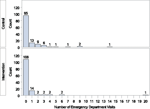
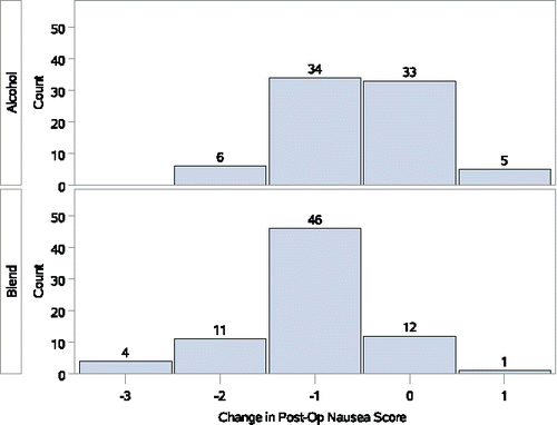
O'Brien and Castelloe (2006) constructed data from a hypothetical study performed by a “Dr. Uri Ologist”, which had equal medians for the two samples being compared, yet the WMW test result was significant. Two real data counterexamples illustrating the same thing are shown in Figure 1 and Figure 2, respectively, and described below.

Figure 1. Emergency department visits in 12 months for the Puff City study.

Figure 2. Changes in postoperative nausea after aromatherapy.

Figure 3. No difference in WMW test, but very different medians.

Figure 4. A difference by WMW test, but very different medians. But in wrong direction!

Figure 5. A global inconsistency.

Counterexample 1: Comparison of two distributions, each with over half their observations equal to 0.

The number of emergency department (ED) visits in the first 12 months postintervention for the two study groups from the Puff City (Joseph et al. 2007) randomized trial of a tailored asthma management program for urban African–American high school students are shown in Figure 1. The majority of students in both groups had no ED visits, resulting in a median of 0 for both groups. However, the proportion with ED visits is only 17.6% for the intervention group versus 26.4% for the control group. The value of ${\widehat{p}}^{\text{'}\text{'}}=\widehat{\mathrm{Pr}}(X_{\mathrm{Intervention}}<X_{\mathrm{Control}})+\widehat{\mathrm{Pr}}(X_{\mathrm{Intervention}}=X_{\mathrm{Control}})/2$ is 0.55 and the WMWodds is 1.21. The Wilcoxon p-value is 0.066, suggesting that there may be a reduction in ED visits with the intervention. The majority of observations, [and hence the sample median(s)] being zero can be quite common when a count variable is analyzed.

Counterexample 2: Comparison of two distributions with equal sample medians, but a very significant WMW test. Figure 2 shows changes in post-operative nausea (PON) scores from two of the groups in a trial of aromatherapy for PON (Hunt et al. 2013). As a brief consideration of the two distributions can show, the WMW significance test result is not a function of the observed medians for the groups being compared. The median PON scores for the alcohol and blend groups are both equal to −1, yet the moderate sample size together with the WMW test p-value of <0.001 implies that there is a large difference between the groups.

Counterexamples 3, 4, and 5 use made up data, but further illustrate the disconnect between medians and WMW tests. (For convenience, the first and second groups will be designated as “A” and “B,” etc., in these examples.)

Counterexample 3: No difference by WMW test, but very different medians

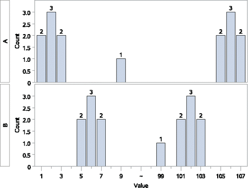
Sample A {1, 1, 2, 2, 2, 3, 3, 9, 105, 105, 106, 106, 106, 107, 107}

Sample B {5, 5, 6, 6, 6, 7, 7, 99, 101, 101, 102, 102, 102, 103, 103}

In this example (Figure 3), the medians are quite different: 9 vs. 99, but otherwise, overall the observations from sample A are no higher or lower than those from sample B. The value of ${\widehat{p}}^{\text{'}\text{'}}=\widehat{\mathrm{Pr}}(X_{\mathrm{A}}<X_{\mathrm{B}})+\widehat{\mathrm{Pr}}(X_{\mathrm{A}}=X_{\mathrm{B}})/2=0.502$, is virtually identical to the null hypothesis value of 0.5, and the WMWodds value is 1.01 despite the very large difference between the medians. Hence, we can have median A << median B, despite a nonsignificant WMW test result (p-value ≅ 1.0).

Counterexample 4: A significant difference by WMW test, and very different medians (but in the wrong direction!)

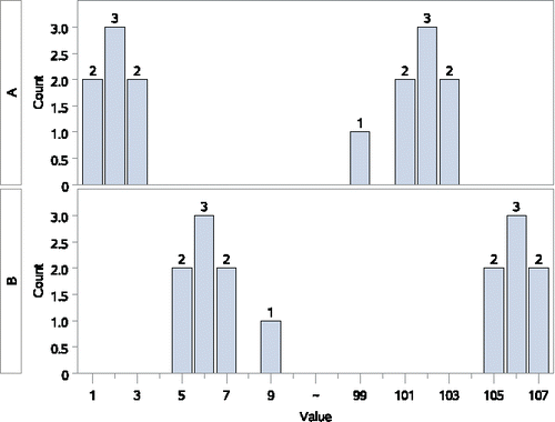
Sample A {1, 1, 2, 2, 2, 3, 3, 99, 101, 101, 102, 102, 102, 103, 103}

Sample B {5, 5, 6, 6, 6, 7, 7, 9, 105, 105, 106, 106, 106, 107, 107}

In this example (Figure 4), the medians are quite different, with the sample A median of 99 being much higher than the sample B median of 9. However, this time, overall the observations from sample A tend to be lower than those from sample B. We have ${\widehat{p}}^{\text{'}\text{'}}=0.716$ and p = 0.046. This example illustrates that we can have median A >> median B, despite a very significant WMW test result that says $\widehat{\mathrm{Pr}}(X_{\mathrm{A}}<X_{\mathrm{B}})+\widehat{\mathrm{Pr}}(X_{\mathrm{A}}=X_{\mathrm{B}})/2=0.72$ is significantly (p = 0.046) greater than the null value of 0.5, and the WMWodds of 2.59 is much greater than the null value of 1.0. Thus, a large median difference can go in the direction opposite of what the WMW test result shows is going on with most of the observations.

Counterexample 5: A global inconsistency for comparisons among several groups

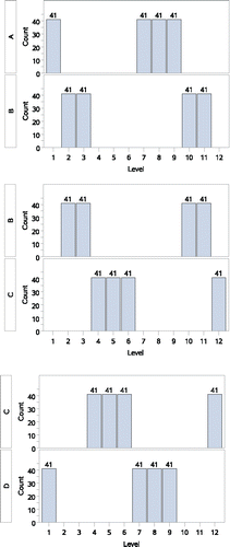
For a final counterexample, we will assume that Dr. Ologist has a colleague, Professor Chase M. Itail, who works with an assistant whose initials are M.C.E. Together, Dr. Itail and his assistant have run a series of experiments comparing four treatment conditions (A, B, C, and D) and they have observed the results shown in Figure 5. Figure 5 (top panel) shows that the distribution of values observed with treatment A are significantly lower than those observed with treatment B. Figure 5 (middle panel) shows that the distribution of values observed with treatment B are significantly lower than those observed with treatment C. Finally, Figure 5 (bottom panel) shows that the distribution of values observed with treatment C are significantly lower than those observed with treatment D. As was shown with the earlier counterexamples, for the A vs. B and B vs. C comparisons, the differences between medians go in a direction opposite that measured and were found significant by the WMW tests. However, this is not the most notable feature of this example.

A comparison of the top panel in Figure 5 (top panel, Group A) and the bottom panel in Figure 5 (bottom panel, Group D) will reveal that they are identical. Thus the comparison of C to D is the same as a comparison of C to A. However, this means that taken as a whole, the WMW test results for this example suggest that Dr. Itail and M.C.E. should arrive at the very counter-intuitive conclusion that A < B < C < A! (Although these results are extremely unintuitive, it is reported that M.C.E. generated an illustration reflecting his interpretation of what the analysis shows. [see http://en.wikipedia.org/wiki/Ascending_and_Descending])

The fundamental feature of the WMW test at play in counterexample 5 is that it measures and reflects an attribute of two sets of observations that is a function of how they are distributed relative to each other, and not of any absolute features of either distribution alone.

Taken together, the above counterexamples clearly illustrate that WMW test results need not correspond to a difference in sample medians. Furthermore, the WMW test results for comparison among several groups need not even be transitive with respect to each other. This is a feature that further reinforces the fact that the test cannot be a direct function of any measure of a sample's central tendency or location. The next section will describe additional circumstances under which the WMW test cannot be assumed to test population medians.

7. Failure (Implausibility and Even Impossibility!) of the Shift Alternative

The assumption of identical distributions that can vary only by a shift in one direction or the other is mathematically convenient, but it can be implausible or even absurd in some of the very situations where the WMW test is most commonly applied. For instance, for a Likert scale outcome where a control population is expected to include some observations that take on the minimum and maximum possible values, a shift of any kind is impossible, since by definition a shift cannot go below the minimum, nor is it able to go above the maximum. Similarly, for an outcome variable, which represents counts of an unfavorable outcome (for instance the number of times pain medication is used), if some subjects with zero instances are expected in the control population, it would be impossible⁴ to improve the distribution by a shift toward lower values in a treated group, since this would imply going below zero.

Even if an ordinal or count outcome distribution had room at either end for an increase or decrease, a shift alternative would require at least one full unit change along the entire distribution. This would often imply a huge and implausible difference between the groups would have to be assumed. Finally, a continuous outcome variable, but one which only takes on positive values cannot be shifted below zero, and a shift of Δ toward higher values would implausibly imply that no values between 0 and Δ will ever be observed for the group shifted higher.

In the next section, we discuss some facts and some conjectures about the persistence of the perception that the WMW procedure tests medians.

8. Why is WMW Testing Misunderstood?

It appears that the origins of misunderstandings about (1) the WMW procedure's relationship to medians, and (2) its validity when applied to data with ties, may be a mixture of both sound and unsound application of historical, pedagogical, mathematical rigor, definitional, practical, and logical considerations.

8.1. Why is the WMW Procedure Commonly Regarded as a Test of Medians?

A simple answer to this question is that it is, in fact a test of medians, if it is assumed that the two populations being compared have identical shapes and that they differ only by a shift alternative. In many cases this assumption of identical shapes and a shift alternative is at least almost true, and therefore the assertion that the WMW procedure tests medians is likely not that far off. Furthermore, when the shift alternative assumption is not almost true, the idea that the WMW procedure tests medians may still have some utility (or at least apparent utility).

We conjecture that since for normally distributed data, means and t-tests are recommended to be reported, and for skewed data, medians and WMW tests are recommended, it is incorrectly assumed that medians and WMW testing go together organically. Also, it may be that since the median is defined as the middlemost of the ranked observations, and the WMW test is a function of ranks, this appears to connect the medians to the Wilcoxon test. (Of course, the ranking within a single group which defines the group's median is different and distinct from the ranking of the combination of two groups that is required to compute the WMW test.)

A major impetus to reporting medians with WMW test results is likely the major utility of reporting a summary statistic that reflects the same scale as the data being analyzed. Of course such utility should not come at the expense of using a summary measure that might lead to misleading inferences.

Finally, the WMW test is commonly regarded as a test of medians because, as O'Brien and Castelloe (2006) note, it is commonly asserted to be so in a number of textbooks. For instance, the following (Newbold and Carlson 2003; LeBlanc 2004; Triola 2006) statements about the Wilcoxon rank sum test were found in a convenient sample of textbooks:

“The null hypothesis is that the two populations have the same median.”

“The two samples come from populations with equal medians.”

“Assuming the null hypothesis that the central locations of the two populations are the same, …”

Another source of instruction about what a WMW test does is data analysis software. Minitab's online support states that the Mann–Whitney test “Determine(s) whether the median of two groups differ when the data for both groups have similarly shaped distributions.” Minitab elsewhere says that “If sampling from nonnormal populations with the same shape and variance, use the Mann–Whitney test,” which implies that Minitab's interpretation for the WMW is relying upon the shift alternative assumption.

It should be noted that while common, the above quotes do not reflect what many others say. Many include much more accurate descriptions of what the WMW test does. One example is Forthofer, Lee, and Hernandez (2007), who stated: “This test is used to determine whether or not the probability that a randomly selected observation from one population is greater than a randomly selected observation from another population is equal to 0.5” (Forthofer, Lee, and Hernandez 2007). Another is the documentation for GraphPad Prism, whose online documentation has a section heading that reads: “The Mann–Whitney test doesn't really compare medians” (see http://www.graphpad.com/guides/prism/5/user-guide/prism5help.html?stat_nonparametric_tests_dont_compa.htm).

8.2. Why Might the WMW Test be Thought to Require Continuous Data?

The answer to this question may come in two parts. The first part is almost certainly historical. That is, before the availability of inexpensive and powerful computing hardware and software, the presence of ties in a dataset could mean that valid WMW testing could be difficult, if not impossible. For small sample sizes (i.e., for which the asymptotic form of the test would be inappropriate), the test had to be performed by calculating a test statistic that was compared to tabled values that were generated assuming continuous data. Since the large number of possible patterns of ties could each require different critical values, generating comprehensive tables for use in WMW testing would be practically impossible.

Pedagogically, if WMW testing is taught starting with a classic table lookup used for smaller sample sizes, and the WMW's asymptotic form for large sample sizes, the former implies that ties will invalidate the tabled critical values, and to an extent that is a function of the number and size of the clumps of ties. Although this problem is obviated by using readily available computer software to compute exact critical values and p-values, it may be that instructors (and some textbook authors) may wish to present only the basic precomputer version of the test. This must become a concern, however, if it is never made clear that the WMW can be valid when implemented using modern computing tools, instead of a manual calculation and table lookup approach. That is, modern computer software can perform an exact WMW test, the equivalent to a table look up, but for any pattern of ties, as long as the sample size is small enough to allow the calculations to be completed in a reasonable amount of time. (If the sample size is large enough to preclude an exact test, it is likely large enough that the asymptotic WMW test may be reliably used.)

The second part of the confusion about the WMW would appear to be conceptual. That is, since the shift alternative formulation of the null and alternative hypotheses for the WMW is inconsistent with ties, a conservative viewpoint based upon the shift alternative might hold that validity of the test with ties is left in doubt. A well-qualified version of this perspective appears to be reflected by Rosner (2016) who stated that “a necessary condition for strict validity of the rank-sum test is that the underlying distributions being compared must be continuous.” Other authors express less qualified uncertainty. For instance, Remington and Schork said “The rank sum should probably not be applied to data with a great many ties, since the derivation of its distributional properties makes no explicit allowance for them” (2000). Even less helpful might be statements in a pair of closely related textbooks, which both give as one of the assumptions underlying the WMW test that “The probability distributions from which the samples are drawn are continuous”, and go on to say: “The (WMW) test is not recommended to compare discrete distributions, for which many ties are expected.” (McClave and Sincich 2013 and McClave et al. 2014⁵.) Finally, it would appear that instead of addressing the issue of ties, one major text (despite containing dozens of pages of detailed and rigorous consideration of the properties of the WMW procedure), simply avoids discussion of ties (Hettmasperger and Mckean 2011).

Finally, it may be that an overabundance of caution might lead some to make a basic logical error: specifically, the “fallacy of the inverse.”⁶ That is, absent awareness of Lehmann's demonstration of the validity of the WMW test with ties, if one is only aware of a derivation based upon the shift alternative, one could go beyond a conservative doubt about the validity of the WMW test with ties, to erroneously denying that validity outright.

9. Teaching Experience

We (ECJ in 2012 and 2014, and AEB in 2013 and 2015) have also lectured on the WMW test in the Biostatistics Methods I at the Colorado School of Public Health, and for 2012 and 2013 conducted pre- and postknowledge surveys. The classes were composed of first year MS students in biostatistics, PhD students in epidemiology, MPH students in applied biostatistics, and students not yet enrolled in any specific program. The results from the pre- and postsurveys are as follows: 63 out of 66 students completed postlecture surveys, and 62 out of 63 correctly picked Pr(X < Y) = 0.5 as the WMW null hypothesis. Forty-four students correctly interpreted the “transitivity” issue, and 45 out of 63 said the WMW portion of the lecture was clear (2 said “not clear”, and 15 said “Not sure”). Twenty-seven students wrote on the postsurvey that the graphical representation of $\widehat{\mathrm{Pr}}$(X < Y) as a bubble plot helped their understanding (see Figure 6).

Figure 6. Bubble plot representing the estimate of p″ = Pr(X₁<X₂) + Pr(X₁ = X₂)/2 for toy example.

10. Graphical Representations of $\widehat{p}=\widehat{\mathrm{Pr}}(X<Y)+\widehat{\mathrm{Pr}}(X=Y)/2$

10.1. Bubble Plot

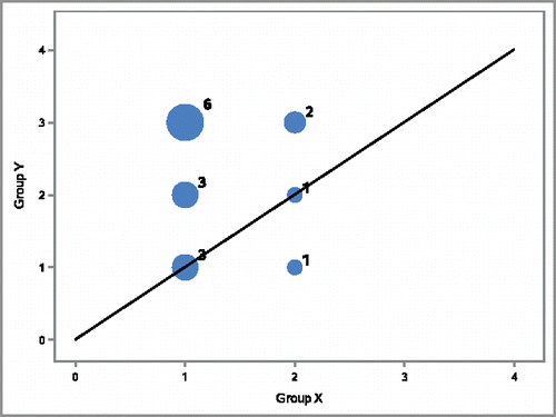
In order to provide a graphical representation of $\widehat{\mathrm{Pr}}$(X < Y) within the time constraints of single lecture, a toy example was used as follows. Let the two sets of observations to be compared be X: (1, 1, 1, 2) and Y: (1, 2, 3, 3). Then all the possible 16 (X,Y) pairs may be enumerated by crossing each value of X with all values of Y as follows. First, listing all pairs with the first value of X (1(1) $$t=\frac{{\bar{x}}_1-{\bar{x}}_2}{\mathrm{se}({\bar{x}}_1-{\bar{x}}_2)}.$$(1) ): (1,1), (1,2), (1,3), (1,3); then the next 2 sets of values are again (1,1), (1,2), (1,3), (1,3), and the last set is (2,1), (2,2), (2,3), (2,3). Figure 1 illustrates these pairs where the size of each bubble represents the number of times that a pair appears in the list of all crossed pairs, for example (1,1) appears three times, and (2,1) only once. To compute $\widehat{\mathrm{Pr}}(X<Y)+\widehat{\mathrm{Pr}}(X=Y)/2$, we calculate the proportion of pairs on the upper part of the graph plus half of the ones on the identity line, giving $\widehat{\mathrm{Pr}}(X<Y)+\widehat{\mathrm{Pr}}(X=Y)/2=\left[6+3+2+\left(4/2\right)\right]/16=13/16=0.8125$. In other words, 13 is the Mann–Whitney U statistic for this comparison, and $\widehat{\mathrm{Pr}}(X<Y)+\widehat{\mathrm{Pr}}(X=Y)/2$ is equal to the proportion of the bubble areas above the line of identity.

Two additional options to graphically display $\widehat{p}$ are an ROC curve and its area, and a “dominance diagram”(Newson 2002).

10.2. ROC Curve Area (the “c-Statistic”)⁷

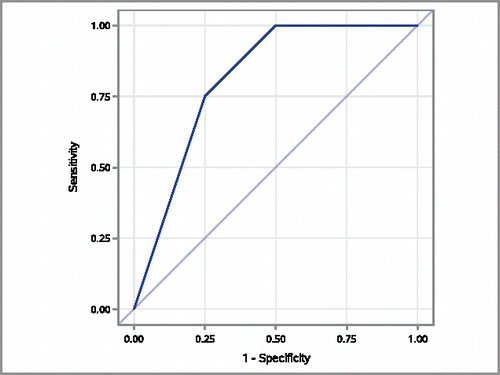
For a potential screening measurement that is either ordinal or continuous, an ROC curve can be used to summarize the ability to discriminate between patients with and without a condition of interest. The sensitivities and specificities are calculated for all possible cut points and sensitivity is plotted on the y-axis and 1—specificity is plotted on the x-axis. The more closely the area under the ROC curve approaches 1.0, the stronger the relationship between the variable and the disease status.

The Roc curve formulation can be generalized to have a connection to the WMW testing situation if the testing problem is thought of as assessing the ability of the outcome variable to distinguish/discriminate between the two groups being compared. The values for the toy example's ROC curve were computed using PROC LOGISTIC in SAS and the curve is shown in Figure 7. An often used interpretation of the area under the ROC curve (AUC) is the proportion of all possible disease/no disease pairs in which the measured variable is higher in the diseased observation than in the nondiseased observation, which is just $\widehat{\mathrm{Pr}}$(X < Y) (Hanley and McNeil 1982). Correspondingly, the WMW statistic can be used to test whether the AUC is significantly different from 0.5 (Bamber 1975). A convenient way to generate a 95% confidence interval for the ROC curve area [and hence Pr(X < Y)] is to use the ROC option in PROC LOGISTIC. For the toy example, the area under the ROC curve is 0.8125 with 95% confidence interval (0.496, 1.000). Since students in an introductory class are often unfamiliar with ROC curves and screening, use of the ROC curve area as a graphical illustration of $\widehat{\mathrm{Pr}}(X<Y)+\widehat{\mathrm{Pr}}(X=Y)/2$ might be best in a class with students who have previously been introduced to ROC curves.

Figure 7. ROC curve area representing the estimate of p″ = Pr(X₁<X₂) + Pr(X₁ = X₂)/2 for toy example.

10.3. Dominance Diagram

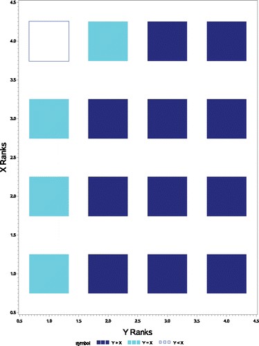
Newson (2002) notes that a “dominance diagram” will also give a graphical representation of $\widehat{\mathrm{Pr}}(X<Y)+\widehat{\mathrm{Pr}}(X=Y)/2$. Figure 8 shows this for the toy example. Roughly speaking, the dominance diagram is a grid displaying the direction for the difference for all combinations of ordered Y and X values (to produce the diagram, ties within the Y and X samples may be broken arbitrarily). As can be seen from the figure, there are 11 solid squares where X < Y and 4 shaded squares where X = Y and again [11 + (4/2)] = 13 is the Mann–Whitney U statistic and $13/16=\widehat{\mathrm{Pr}}(X<Y)+\widehat{\mathrm{Pr}}(X=Y)/2$. (The dominance diagram is probably a bit more complex than the bubble plot shown earlier, but it does not require additional concepts as are required for an ROC curve, so it may be a viable option for some classes.)

Figure 8. Dominance diagram representing the estimate of p″ = Pr(X₁<X₂) + Pr(X₁ = X₂)/2 for toy example.

11. Discussion

It logically follows that the imperfect connection of the WMW test to medians will imply that use of the Hodges-Lehmann confidence interval for a difference in locations (as reflected by the medians) may also perform poorly. For instance, for the aromatherapy example (which has a moderate sample size), the exact Hodges–Lehmann confidence interval computed by SAS goes from −1 to 0, which seems inconsistent with a p-value that is far into the rejection region. While a comprehensive presentation about the WMW test may need to cover related procedures like Hodges–Lehmann, it is desirable to make sure students are aware of its limitations.

To further emphasize the importance of Pr(X < Y) as central to the WMW test, this quantity must be used if calculation of sample size or power is required. Basic formulas for these were shown by Zhou et al. (2008) and Divine et al. (2010) and very reliable sample size and power computations can be made using PROC POWER in SAS or using nQuery Advisor.

It is beyond the scope of this article,⁸ but it should be noted that the Wilcoxon signed rank test has a similarly poor connection to the sample median, despite what may be asserted in textbooks. Again counterexamples are relatively easy to find. [Unfortunately, the quantity that the signed rank test is a function of: Pr[X₁ + X₂ < 0], is not as interpretable as Pr(X < Y) is for the WMW test, and the relationship is only asymptotic.]

12. Summary

We have shown by use of both real data and constructed counterexamples that the WMW test is in no way a function of the observed sample medians. It has also been illustrated that its intended connection to a comparison of underlying population medians can be impossible or at least implausible in many common situations where the test is applied. Empirically, the WMW test should be regarded as a test of the null hypothesis that Pr(X < Y) + Pr(X = Y)/2 = 0.5, where X and Y are random observations from the two populations being compared. Finally, despite misleading or ambiguous statements in some textbooks, validity of the WMW test does not require continuous data.

Supplementary Materials

The online supplementary materials contain the counterexamples presented in the article, and the SAS programs.

Acknowledgments

The authors are grateful to Elizabeth Stewart (Henry Ford Hospital) for help with formatting, to Elizabeth Furest (Henry Ford Hospital) for editorial assistance, and to the referees and editors for their careful review and comments.

Notes

¹ $\widehat{\mathrm{Pr}}(X_1<X_2)+\widehat{\mathrm{Pr}}(X_1=X_2)/2$ represents the sample estimate. (For instance U/n₁n₂, for the Mann–Whitney formulation.) For the underlying population quantity: p′′ = Pr(X₁ < X₂) + Pr(X₁ = X₂)/2, the evaluation is over all possible values of X₁ and X₂. (For continuous distributions Pr(X₁ = X₂)/2 is equal to 0.)

2 The computing formula is different, but to a close approximation, if D is the number of different levels observed and P_c is the proportion of observations tied at the cth level, the ties adjusted variance is equal to $(1-{\sum }_{c=1}^D{P_c}^3)$ times the variance without ties.

3 More formally, Lehmann states the condition as the “max (d_i/N) is bounded away from 1 as N tends to infinity.” Or that there exists a positive number ϵ < 1, such that for all i, d_i/N <= 1 - ϵ, where the d_i are the numbers of observations tied at each possible value. (The sum d₁ + ⋅⋅⋅ + d_e = N.)

4 Reiczige et al. (2005) called such a shift “simply nonsense” for their example of parasite infection counts.

5 This edition includes a somewhat qualifying footnote, which reads: “^*Adjustments for ties are available with the Wilcoxon rank sum test. Consult the references at the end of this chapter.” (Presumably the newest (2017) edition of the other McClave and Sincich, text has the same qualifier.)

6 The basic form of the fallacy is given “If A then B” and not A, erroneously concluding not B. In this case A would be “the shift alternative holds” and B would be “the WMW test is valid.”

7 In the rare situation (for instance due to one or more extreme outliers) when the differences between the raw means and the mean ranks go in different directions, $\widehat{\mathrm{Pr}}$(X < Y) will be equal to 1 – c, instead of being equal to c.

8 More discussion about the WMW and Wilcoxon signed rank tests can be found in Divine et al. (2013).

References

- Agresti, A. (1980), “Generalized Odds Ratios for Ordinal Data,” Biometrics, 36, 59–67.
- Bamber, D. (1975), “The Area Above the Ordinal Dominance Graph and the Area Below the Receiver Operating Characteristic Graph,” Journal of Mathematical Psychology, 12, 387–415.
- Brunner, E., and Munzel, U. (2000), “The Nonparametric Behrens-Fisher Problem: Asymptotic Theory and a Small-Sample Approximation,” Biometrical Journal, 42, 17–25.
- Delaney, H. D., and Vargha, A. (2002), “Comparing Several Robust Tests of Stochastic Equality Withordinally Scaled Variables and Small to Moderate Sample Sizes,” Psychological Methods, 7, 485–503.
- Divine, G., Kapke, A., Havstad, S., and Joseph, C. (2010), “Exemplary Data Set Sample Size Calculation for Wilcoxon–Mann–Whitney Tests,” Statistics in Medicine, 29, 108–115.
- Divine, G., Norton, H., Hunt, R., and Dienemann, J. (2013), “A Review of Analysis and Sample Size Calculation Considerations for Wilcoxon Tests,” Anesthesia & Analgesia, 117, 699–710.
- Fligner, M. A., and Policello, G. E. (1981), “Robust Rank Procedures for the Behrens-Fisher Problem,” Journal of the American Statistical Association, 76, 162–168.
- Forthofer, R., Lee, E., and Hernandez, M. (2007), Biostatistics: A Guide to Design, Analysis, and Discovery (2nd ed.), Amsterdam: Elsevier Academic Press.
- Hanley, J., and McNeil, B. (1982), “The Meaning and Use of the Area Under a Receiver Operating Characteristic (ROC) Curve,” Radiology, 143, 29–36.
- Hettmansperger, T. P., and McKean, J. W. (2011), Robust nonparametric Statistical Methods (2nd ed.), Boca Raton, FL: CRC Press.
- Hunt, R., Dienemann, J., Norton, H., Hartley, W., Hudgens, A., Stern, T., and Divine, G. (2013), “Aromatherapy as Treatment for Postoperative Nausea,” Anesthesia & Analgesia, 117, 597–604.
- Joseph, C., Peterson, E., Havstad, S., Johnson, C., Hoerauf, S., Stringer, S., and Strecher, V. (2007), “A Web-Based, Tailored Asthma Management Program For Urban African-American High School Students,” American Journal of Respiratory and Critical Care Medicine, 175, 888–895.
- LeBlanc, D. (2004), Statistics: Concepts and Applications for Science, Boston, MA: Jones and Bartlett.
- Lehmann, E. L. (1975), Nonparametrics: Statistical Methods Based on Ranks, San Francisco, CA: Holden-Day, Inc., 480 S.
- McClave, J. T., and Sincich, T. T. (2013), Statistics (13th ed.), New York: Pearson.
- McClave, J. T., Benson, P. G., and Sincich, T. T. (2014), Statistics for Economics and Business (12th ed.), New York: Pearson.
- Newbold, P., and Carlson, W. (2003), Statistics for Business and Economics (5th ed.), Upper Saddle River, N.J.: Pearson Prentice Hall.
- Newson, R. (2002), “Parameters Behind “Nonparametric” Statistics: Kendall's tau, Somers' D and Median Differences,” Stata, 2, 45–64.
- O'Brien, R. G. and Castelloe, J. M. (2006), Proceedings of the Thirty-first Annual SAS Users Group International Conference, Paper 209-31. Cary, NC: SAS Institute Inc;. Exploiting the Link between the Wilcoxon–Mann–Whitney Test and a Simple Odds Statistic. 31st Annual SAS Users Group International Conference. Lecture conducted from, Cary, NC. Available at http://www2.sas.com/proceedings/sugi31/209-31.pdf
- Reiczigel, J., Zakariá, I., and Rózsa, L. (2005), “A Bootstrap Test of Stochastic Equality of Two Populations,” The American Statistician, 59, 156–161.
- Rosner, B. (2016), Fundamentals of Biostatistics, (8th ed.), Boston, MA: Cengage Learning.
- Pratt, J. (1964), “Robustness of Some Procedures for the Two-Sample Location Problem,” Journal of the American Statistical Association, 59, 665–680.
- Triola, M. and Triola, M. (2006), Biostatistics for the Biological and Health Sciences. Boston, MA: Pearson Addison-Wesley.
- Zhao, Y., Rahardja, D., and Qu, Y. (2008), “Sample Size Calculation for the Wilcoxon–Mann–Whitney Test Adjusting for Ties,” Statistics in Medicine, 27, 462–468.