Bayesian Analysis on a Noncentral Fisher–Student’s Hypersphere

ABSTRACT

Fisher succeeded early on in redefining Student’s t-distribution in geometrical terms on a central hypersphere. Intriguingly, a noncentral analytical extension for this fundamental Fisher–Student’s central hypersphere h-distribution does not exist. We therefore set to derive the noncentral h-distribution and use it to graphically illustrate the limitations of the Neyman–Pearson null hypothesis significance testing framework and the strengths of the Bayesian statistical hypothesis analysis framework on the hypersphere polar axis, a compact nontrivial one-dimensional parameter space. Using a geometrically meaningful maximal entropy prior, we requalify the apparent failure of an important psychological science reproducibility project. We proceed to show that the Bayes factor appropriately models the two-sample t-test p-value density of a gene expression profile produced by the high-throughput genomic-scale microarray technology, and provides a simple expression for a local false discovery rate addressing the multiple hypothesis testing problem brought about by such a technology.

KEYWORDS:

• Confidence intervals
• Bayesian prior
• Bayesian credible intervals
• Multiple hypothesis testing
• Local false discovery rate

1. Introduction

The statistical analysis literature is replete with words of caution on the use and misuse of various statistical hypothesis testing methods, the contrasted discourse about a much used but heavily criticized Neyman–Pearson null hypothesis significance testing (NHST) framework and a powerful but yet to be fully embraced Bayesian hypothesis testing framework being particularly notorious. See, for example, Greenland et al. (2016), Rothman (2016), Wasserstein and Lazar (2016), and references therein for an all encompassing scope. See also Goodman (1999a, 1999b) for a more restricted point of view on medical statistics. Our contribution to this debate is meant to be modest and focused: we shall recast the classical two-sample t-test in an intuitive geometrical setting so as to allow the reader to assess the respective strengths and weaknesses of the NHST and Bayesian frameworks through informative graphical representations on a compact nontrivial one-dimensional parameter space. The practical examples chosen will be drawn from the biomedical research realm which is undergoing major conceptual shifts in data analysis, partly in response to the creation of genomic-scale high-throughput technologies, partly in response to a science reproducibility problem.

Many authors have commented on the elegance and simplicity of geometrical approaches to statistics. In their paper entitled ‘The geometry of estimation’, Durbin and Kendall (1951) state:

“In the ultimate analysis geometrical ‘proofs’ in more than three dimensions are only restatements of analytical results in a special language; but they are nevertheless very useful, partly because of their elegance and partly because they carry a greater degree of conviction and understanding, to some minds at least, than the analytical approach. They also suggest generalizations (...).”

Sir Ronald Fisher was among those advocating early on a geometrical approach to statistics. Historical accounts narrate how he cleanly redefined Student’s t-distribution on a hypersphere (Gorroochurn 2016). It is therefore intriguing that one cannot find any trace in the literature of a noncentral analytical extension for the fundamental Fisher–Student’s central hypersphere distribution, as such an extension could ease illustration of the strengths of the Bayesian framework on the hypersphere polar axis, a compact nontrivial one-dimensional parametric space. Instead, one still has to rely on an unwieldy noncentral t-distribution which has obfuscated such an endeavour till now.

The geometrical framework herein advocated will allow us to: reexpress Student’s t-distribution as the Fisher–Student’s central hypersphere h-distribution, derive its analytical noncentral extension, and compare the analytical noncentral h-distribution to the unwieldy noncentral t-distribution in Section 2; graphically compare over compact domains the NHST and Bayesian hypothesis testing frameworks in Sections 3 and 4; explore graphically how the Bayesian framework interprets the apparent failure of an important psychological science reproducibility project, fares when analyzing a gene expression profile microarray dataset, and provides a simple expression for a local false discovery rate addressing the multiple hypothesis testing problem in Section 5.

In order not to distract the reader, our argumentation will mostly consist of statements without extensive proofs. The reader is referred to the Appendices for details.

2. Noncentral Hypersphere h-distribution

Consider an experiment consisting of measuring one continuous outcome in two different experimental conditions, n₁ times for the first condition, n₂ for the second condition. The result of such an experiment can be collated into an observation vector $\mathbf{o}=\left(\begin{array}{c}{\mathbf{o}}_1\\ {\mathbf{o}}_2\end{array}\right)$ of length N = n₁ + n₂. The observation vector o can be projected on the overall center-of-mass C, the between-class variance hyperplane B, and the within-class variance hyperplane W using the matrix projectors P_C, P_B, and P_W defined in Appendix A. In both projection and trigonometric terms, the two-sample t-statistic is defined as the signed squared root of the variance ratio (1) $$\begin{array}{ccc}\hfill t& =& {\left[\nu \frac{{\mathbf{o}}^t{P}_B\mathbf{o}}{{\mathbf{o}}^t{P}_W\mathbf{o}}\right]}^{1/2}=\sqrt{\nu }\frac{cos\theta }{sin\theta },\hfill \\ & & -\infty \le t\le \infty ,0\le \theta \le \pi ,\nu =N-2.\hfill \end{array}$$(1) For the two-sample case, the matrix projector P_B has rank one and can be expanded as P_B = T_BT^t_B, where the relevant eigenvector (2) $${\mathbf{T}}_B=\frac{1}{\sqrt{\frac{1}{n_1}+\frac{1}{n_2}}}\left(\begin{array}{c}\phantom{-}\frac{{\mathbf{1}}_{n_1}}{n_1}\\ -\frac{{\mathbf{1}}_{n_2}}{n_2}\end{array}\right)=\frac{1}{\sqrt{2n}}\left(\begin{array}{c}\phantom{-}{\mathbf{1}}_n\\ -{\mathbf{1}}_n\end{array}\right)\text{if}{n}_1=n_2=n,$$(2) allows computation to within a constant of the difference of means between the two experimental conditions. In the following, T_B will be referred to as the unit polar axis of the hypersphere under consideration. When the random observation vector o distributes according to a maximal entropy equiprobability distribution on the unit radius hypersphere ${\mathcal{S}}^{\nu }$—arguably one of the most important continuous distributions in probability theory—its projection cos θ = T^t_Bo on the polar axis distributes according to the Fisher–Student’s central h-distribution (3) $${\rho }_{(\nu ,0)}\left(\theta \right)=\frac{\Gamma \left(\frac{\nu +1}{2}\right)}{\Gamma \left(\frac{1}{2}\right)\Gamma \left(\frac{\nu }{2}\right)}{sin}^{\nu -1}\theta ,0\le \theta \le \pi ,$$(3) (Fisher et al. 1925). This distribution will stand hereafter for the null hypothesis H_o. The central h-distribution is symmetrical upon reflection across the equatorial midline at cos θ = 0, and its width narrows as ν increases, an intrinsic geometrical property of high-dimensional hyperspheres which pack most of their surface on their equatorial bulge. The null index in the parameter set (ν, δ = 0) refers to the fact that, for a central distribution, the noncentrality parameter δ—to be formally introduced below—is zero. Poincaré’s lemma states that ρ_{(ν, 0)}(θ) converges to the normal distribution as ν goes to infinity (Mazliak 2015). Computation of the cumulative distribution functions and, consequently, of p-values for the central hypersphere distribution (3(3) $${\rho }_{(\nu ,0)}\left(\theta \right)=\frac{\Gamma \left(\frac{\nu +1}{2}\right)}{\Gamma \left(\frac{1}{2}\right)\Gamma \left(\frac{\nu }{2}\right)}{sin}^{\nu -1}\theta ,0\le \theta \le \pi ,$$(3) ) can be carried out analytically: see Appendix D.

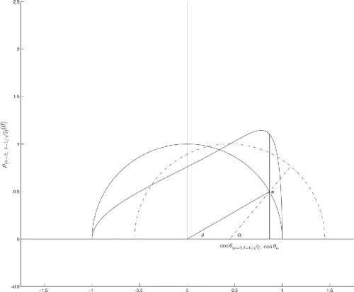
Figure 1. Translated and noncentral hypersphere distribution. The silhouetted hypersphere ${\mathcal{S}}^{\nu =2}$ is translated by a normalized effect size $\delta =1/\sqrt{2}$ — re-expressed in geometrical terms as $cos{\theta }_{(\nu ,\delta )}=\delta /\sqrt{{\delta }^2+\nu }{\mid }_{(\nu =2,\delta =1/\sqrt{2})}=1/\sqrt{5}$ — along the horizontal polar axis. All experimental measurements are expressed in terms of the polar angle θ, which relates to the null hypothesis H_o hypersphere ρ_{(ν, δ = 0)}(θ) centered on the origin. The angle Θ for its part relates to measurements which can be made in the intrinsic reference system centered on the round dashed translated hypersphere. As the angle Θ rotates from 0 to π, the translated symmetrical hypersphere is mapped vertically above the observation’s projection cos θ_o on the unsymmetrical noncentral h-distribution ${\rho }_{(\nu =2,\delta =1/\sqrt{2})}^h\left(\theta \right)$ of interest.

We now extend the Fisher–Student’s central h-distribution (3(3) $${\rho }_{(\nu ,0)}\left(\theta \right)=\frac{\Gamma \left(\frac{\nu +1}{2}\right)}{\Gamma \left(\frac{1}{2}\right)\Gamma \left(\frac{\nu }{2}\right)}{sin}^{\nu -1}\theta ,0\le \theta \le \pi ,$$(3) ) to that of a noncentral h-distribution with center-of-mass shifted away from the origin of the referential system by the value of the noncentrality parameter δ. In geometric terms, the t-like noncentrality parameter δ defines the angle $cot{\theta }_{(\nu ,\delta )}=\delta /\sqrt{\nu }$ which imparts to the hypersphere the translation given by (4) $$cos{\theta }_{(\nu ,\delta )}=\frac{\delta /\sqrt{\nu }}{\sqrt{{(\delta /\sqrt{\nu })}^2+1}}=\frac{\delta }{\sqrt{{\delta }^2+\nu }}$$(4) on the finite cosine range − 1 ⩽ cos θ ⩽ 1 along the polar axis T_B defined in equation (2(2) $${\mathbf{T}}_B=\frac{1}{\sqrt{\frac{1}{n_1}+\frac{1}{n_2}}}\left(\begin{array}{c}\phantom{-}\frac{{\mathbf{1}}_{n_1}}{n_1}\\ -\frac{{\mathbf{1}}_{n_2}}{n_2}\end{array}\right)=\frac{1}{\sqrt{2n}}\left(\begin{array}{c}\phantom{-}{\mathbf{1}}_n\\ -{\mathbf{1}}_n\end{array}\right)\text{if}{n}_1=n_2=n,$$(2) ). As represented in Figure 1, angular measurements are affected by the translation. In the referential system centered on the translated hypersphere, the cotangent of the polar angle is given by $$cot{\Theta }_{(\nu ,\delta )}\left(\theta \right)=\frac{cos\theta -cos{\theta }_{(\nu ,\delta )}}{sin\theta }$$reminiscent of the z-score (x − μ)/σ for a normal distribution with non-vanishing mean μ, from which one computes the transformation angle (5) $${\Theta }_{(\nu ,\delta )}\left(\theta \right)=\text{arccot}\left(\frac{cos\theta -cos{\theta }_{(\nu ,\delta )}}{sin\theta }\right).$$(5) In the translated referential system, the central h-distribution provided by equation (3(3) $${\rho }_{(\nu ,0)}\left(\theta \right)=\frac{\Gamma \left(\frac{\nu +1}{2}\right)}{\Gamma \left(\frac{1}{2}\right)\Gamma \left(\frac{\nu }{2}\right)}{sin}^{\nu -1}\theta ,0\le \theta \le \pi ,$$(3) ) holds, not unlike the shape of a normal distribution left unchanged by a simple translation as graphically represented in Figure 1. In the original referential system, the noncentral h-distribution transforms according to the change of variable (5(5) $${\Theta }_{(\nu ,\delta )}\left(\theta \right)=\text{arccot}\left(\frac{cos\theta -cos{\theta }_{(\nu ,\delta )}}{sin\theta }\right).$$(5) ): one finds (6) $$\begin{array}{ccc}\hfill {\rho }_{(\nu ,\delta )}^h\left(\theta \right)& =& {\rho }_{(\nu ,0)}\left({\Theta }_{(\nu ,\delta )}\left(\theta \right)\right)\frac{d{\Theta }_{(\nu ,\delta )}\left(\theta \right)}{d\theta }\hfill \\ & =& \frac{\Gamma \left(\frac{\nu +1}{2}\right)}{\Gamma \left(\frac{1}{2}\right)\Gamma \left(\frac{\nu }{2}\right)}{sin}^{\nu -1}{\Theta }_{(\nu ,\delta )}\left(\theta \right)J_{(\nu ,\delta )}\left(\theta \right),\hfill \end{array}$$(6) where the transformation’s Jacobian is given by $$J_{(\nu ,\delta )}\left(\theta \right)=\frac{d{\Theta }_{(\nu ,\delta )}\left(\theta \right)}{d\theta }=\frac{1-cos\theta cos{\theta }_{(\nu ,\delta )}}{[1-2cos\theta cos{\theta }_{(\nu ,\delta )}+{cos}^2{\theta }_{(\nu ,\delta )}]}.$$The various terms of the h-distribution (6(6) $$\begin{array}{ccc}\hfill {\rho }_{(\nu ,\delta )}^h\left(\theta \right)& =& {\rho }_{(\nu ,0)}\left({\Theta }_{(\nu ,\delta )}\left(\theta \right)\right)\frac{d{\Theta }_{(\nu ,\delta )}\left(\theta \right)}{d\theta }\hfill \\ & =& \frac{\Gamma \left(\frac{\nu +1}{2}\right)}{\Gamma \left(\frac{1}{2}\right)\Gamma \left(\frac{\nu }{2}\right)}{sin}^{\nu -1}{\Theta }_{(\nu ,\delta )}\left(\theta \right)J_{(\nu ,\delta )}\left(\theta \right),\hfill \end{array}$$(6) ) can be regrouped such that the noncentral h-distribution simply reads (7) $${\rho }_{(\nu ,\delta )}^h\left(\theta \right)={\mathcal{L}}_{(\nu ,\delta )}^h\left(\theta \right){\rho }_{(\nu ,0)}\left(\theta \right),$$(7) where the multiplicative function ${\mathcal{L}}_{(\nu ,\delta )}^h\left(\theta \right)$—readily interpreted as the likelihood ratio between the noncentral ρ^h_{(ν, δ)} and central ρ_{(ν, 0)} h-distributions—is given by (8) $${\mathcal{L}}_{(\nu ,\delta )}^h\left(\theta \right)=\frac{1-cos\theta cos{\theta }_{(\nu ,\delta )}}{{[1-2cos\theta cos{\theta }_{(\nu ,\delta )}+{cos}^2{\theta }_{(\nu ,\delta )}]}^{\frac{\nu +1}{2}}}.$$(8) Since the hypersphere dimensional parameter ν is usually prespecified by the experimental setup, the noncentral h-distribution is essentially parameterized by the noncentrality parameter δ as reexpressed in geometrical terms in Equation (4(4) $$cos{\theta }_{(\nu ,\delta )}=\frac{\delta /\sqrt{\nu }}{\sqrt{{(\delta /\sqrt{\nu })}^2+1}}=\frac{\delta }{\sqrt{{\delta }^2+\nu }}$$(4) ). Compare with Gönen et al. (2005) and Wang and Liu (2016). When δ = 0, cos θ_{(ν, δ)} = 0, and ρ^h_{(ν, δ = 0)}(θ) simplifies to the Fisher–Student’s central h-distribution ρ_{(ν, 0)}(θ), as expected. From its definition in Equation (6(6) $$\begin{array}{ccc}\hfill {\rho }_{(\nu ,\delta )}^h\left(\theta \right)& =& {\rho }_{(\nu ,0)}\left({\Theta }_{(\nu ,\delta )}\left(\theta \right)\right)\frac{d{\Theta }_{(\nu ,\delta )}\left(\theta \right)}{d\theta }\hfill \\ & =& \frac{\Gamma \left(\frac{\nu +1}{2}\right)}{\Gamma \left(\frac{1}{2}\right)\Gamma \left(\frac{\nu }{2}\right)}{sin}^{\nu -1}{\Theta }_{(\nu ,\delta )}\left(\theta \right)J_{(\nu ,\delta )}\left(\theta \right),\hfill \end{array}$$(6) ), integration of the noncentral h-distribution ρ^h_{(ν, δ)}(θ) between any integration bounds is given by $${\int }_{{\theta }_1}^{{\theta }_2}{\rho }_{(\nu ,\delta )}^h\left(\theta \right)d\theta ={\int }_{{\Theta }_{(\nu ,\delta )}\left({\theta }_1\right)}^{{\Theta }_{(\nu ,\delta )}\left({\theta }_2\right)}{\rho }_{(\nu ,0)}\left(\Theta \right)d\Theta ,$$that is, integration of the noncentral h-distribution between the integration bounds [θ₁, θ₂] simply boils down to integration of Student’s distribution (3(3) $${\rho }_{(\nu ,0)}\left(\theta \right)=\frac{\Gamma \left(\frac{\nu +1}{2}\right)}{\Gamma \left(\frac{1}{2}\right)\Gamma \left(\frac{\nu }{2}\right)}{sin}^{\nu -1}\theta ,0\le \theta \le \pi ,$$(3) ) between the transformed integration bounds [Θ_{(ν, δ)}(θ₁), Θ_{(ν, δ)}(θ₂)] provided by Equation (5(5) $${\Theta }_{(\nu ,\delta )}\left(\theta \right)=\text{arccot}\left(\frac{cos\theta -cos{\theta }_{(\nu ,\delta )}}{sin\theta }\right).$$(5) ). All the relevant integrations have been carried out analytically and the results are provided in Appendix D. For the sake of completeness, we state without proof that the noncentral t-distribution function—formally derived through introduction of the ratio of a random variable distributing according to a normal distribution $\mathcal{N}(\delta ,1)$ over a random variable distributing according to a χ_ν distribution—can similarly be rewritten $${\rho }_{(\nu ,\delta )}^t\left(\theta \right)={\mathcal{L}}_{(\nu ,\delta )}^t\left(\theta \right){\rho }_{(\nu ,0)}\left(\theta \right),0\le \theta \le \pi ,$$where the likelihood ratio ${\mathcal{L}}_{(\nu ,\delta )}^t\left(\theta \right)$ is given by $$\begin{array}{ccc}\hfill {\mathcal{L}}_{(\nu ,\delta )}^t\left(\theta \right)& =& \frac{e^{-\frac{{\delta }^2}{2\phantom{{}^2}}}}{\Gamma \left(\frac{\nu +1}{2}\right)}{\int }_0^{\infty }{e}^{-v}{e}^{(\sqrt{2}\delta cos\theta )v^{\frac{1}{2}}}{v}^{\frac{\nu -1}{2}}dv\hfill \\ & =& e^{-\frac{{\delta }^2}{2\phantom{{}^2}}}\sum _{j=0}^{\infty }\frac{\Gamma \left(\frac{j+\nu +1}{2}\right)}{\Gamma \left(\frac{\nu +1}{2}\right)}\frac{{(\sqrt{2}\delta cos\theta )}^j}{j!}\hfill \end{array}$$after expansion of the exponential and use of the gamma function definition. The likelihood ratio ${\mathcal{L}}_{(\nu ,\delta )}^t\left(\theta \right)$ thus involves a cumbersome sum over an infinite number of terms. When δ = 0, ${\mathcal{L}}_{(\nu ,0)}^t\left(\theta \right)=1,$ and the noncentral t-distribution ρ^t_{(ν, δ)}(θ) simplifies to on the Fisher–Student’s central h-distribution ρ_{(ν, 0)}(θ), as expected.

To summarize, the noncentral h-distribution ρ^h_{(ν, δ)}(θ) is obtained by translating the Fisher–Student’s central h-distribution (3(3) $${\rho }_{(\nu ,0)}\left(\theta \right)=\frac{\Gamma \left(\frac{\nu +1}{2}\right)}{\Gamma \left(\frac{1}{2}\right)\Gamma \left(\frac{\nu }{2}\right)}{sin}^{\nu -1}\theta ,0\le \theta \le \pi ,$$(3) ) along the polar axis T_B, while the noncentral t-distribution ρ^t_{(ν, δ)}(θ) is obtained as the marginal of the joint probability of a normal distribution $\mathcal{N}(\delta ,1)$ 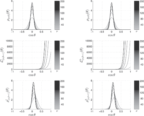times a χ²_ν distribution: the noncentral h-distribution is thus both conceptually and analytically simpler. Furthermore, while both noncentral h- and t-distributions simplify to the Fisher–Student’s central h-distribution when δ = 0, it can be graphically ascertained that, for a nonvanishing value of δ, ρ^h_{(ν, δ)}(θ) and ρ^t_{(ν, δ)}(θ) are almost superposable, as graphically demonstrated in Figure 2. We are thus justified to use the closed analytical form (7(7) $${\rho }_{(\nu ,\delta )}^h\left(\theta \right)={\mathcal{L}}_{(\nu ,\delta )}^h\left(\theta \right){\rho }_{(\nu ,0)}\left(\theta \right),$$(7) ) for noncentral h-distribution ρ^h_{(ν, δ)}(θ)—with its analytical and readily factorized likelihood ratio (8(8) $${\mathcal{L}}_{(\nu ,\delta )}^h\left(\theta \right)=\frac{1-cos\theta cos{\theta }_{(\nu ,\delta )}}{{[1-2cos\theta cos{\theta }_{(\nu ,\delta )}+{cos}^2{\theta }_{(\nu ,\delta )}]}^{\frac{\nu +1}{2}}}.$$(8) )—in order to exploit the Bayesian framework to its fullest in the following. Finally, a most instructive generalization to the noncentral F-distribution is to be found in Appendix C.

Figure 2. Noncentral t-distributions on the left and h-distributions on the right for a varying number of degrees of freedom—or, equivalently, hypersphere dimension—ν which can be deduced from the grayscale colorbars. The Fisher–Student’s central hypersphere distribution is given in duplicate in the upper panels. The likelihood ratios ${\mathcal{L}}_{(\nu ,\delta )}^t\left(\theta \right)$ and ${\mathcal{L}}_{(\nu ,\delta )}^h\left(\theta \right)$ for δ = 1 are given in the middle left and right panels, respectively. The noncentral ρ^t_{(ν, δ)}(θ) and ρ^h_{(ν, δ)}(θ) distributions, products of the two functions above them, are given in the lower left and right panels, respectively. The resulting distributions are almost superposable.

3. Null Hypothesis Significance Testing Framework

We shall refer in the following to δ as the normalized effect size, and to Δ as the sampling distribution noncentrality parameter. The latter is determined in Appendix B in geometric terms. We shall abide with the convention of using the Greek letters δ or Δ to designate the distributions’ noncentrality parameters, and the roman letters d or D to designate their respective estimates (Cumming and Finch 2001).

The Neyman–Pearson NHST framework calls for rejection of the null hypothesis δ = 0 whenever the observed p-value established with respect to the central hypersphere distribution ρ_{(ν, 0)}(θ) is less than or equal to a pre-chosen Type I error (false positive) level α. For the hypersphere distribution of interest, the NHST prescription requires specification of the statistical test specificity at Type I error (false positive) level α $$\text{specificity}=1-\alpha =1-{\int }_0^{{\theta }_{\alpha }}{\rho }_{(\nu ,0)}\left(\theta \right)d\theta =1-p\left({\theta }_{\alpha }\right)$$in terms of the central h-distribution (3(3) $${\rho }_{(\nu ,0)}\left(\theta \right)=\frac{\Gamma \left(\frac{\nu +1}{2}\right)}{\Gamma \left(\frac{1}{2}\right)\Gamma \left(\frac{\nu }{2}\right)}{sin}^{\nu -1}\theta ,0\le \theta \le \pi ,$$(3) ), equation which determines the one-tail statistical critical angle $cot{\theta }_{\alpha }=t_{\alpha }/\sqrt{\nu },$ reciprocally related to the sensitivity (power to detect the effect size) at type II error (false negative) level β $$\begin{array}{ccc}\hfill \text{sensitivity}& =& 1-\beta ={\int }_0^{{\theta }_{\alpha }}{\rho }_{(\nu ,\Delta )}^h\left(\theta \right)d\theta \hfill \\ & =& {\int }_0^{{\Theta }_{(\nu ,\Delta )}\left({\theta }_{\alpha }\right)}{\rho }_{(\nu ,0)}\left(\Theta \right)d\Theta =p\left({\Theta }_{(\nu ,\Delta )}\left({\theta }_{\alpha }\right)\right)\hfill \end{array}$$in terms of the noncentral h-distribution (7(7) $${\rho }_{(\nu ,\delta )}^h\left(\theta \right)={\mathcal{L}}_{(\nu ,\delta )}^h\left(\theta \right){\rho }_{(\nu ,0)}\left(\theta \right),$$(7) ). Figure 3 graphically summarizes these concepts on the finite polar axis. In the frequentist framework, the t-statistic (1(1) $$\begin{array}{ccc}\hfill t& =& {\left[\nu \frac{{\mathbf{o}}^t{P}_B\mathbf{o}}{{\mathbf{o}}^t{P}_W\mathbf{o}}\right]}^{1/2}=\sqrt{\nu }\frac{cos\theta }{sin\theta },\hfill \\ & & -\infty \le t\le \infty ,0\le \theta \le \pi ,\nu =N-2.\hfill \end{array}$$(1) ) provides a maximum likelihood estimate D for Δ. Similarly, the correlation-like projection cos θ = T^t_Bo provides a maximum likelihood estimate for (9) $$cos{\theta }_{(\nu ,\Delta )}=\frac{\Delta /\sqrt{\nu }}{\sqrt{{(\Delta /\sqrt{\nu })}^2+1}}=\frac{\Delta }{\sqrt{{\Delta }^2+\nu }}.$$(9) See Appendix B for various relationships between Δ, δ, ν and the two-sample sizes (n₁, n₂). In order to compute a confidence interval (CI) for the estimate cos θ_{(ν, D)}, one needs to be able to express θ in terms of Θ. Solving a quadratic equation, one finds $$cos\theta \left(\Theta \right)={sin}^2\Theta cos{\theta }_{(\nu ,D)}\pm cos\Theta \sqrt{1-{sin}^2\Theta {cos}^2{\theta }_{(\nu ,D)}}.$$Using the latter, the two-tail confidence interval for cos θ_{(ν, D)} is found to be given by (10) $$\begin{array}{ccc}\hfill cos{\theta }_{(\nu ,D)}{\text{CI}}_{1-\alpha }& =& {sin}^2{\theta }_{\alpha /2}cos{\theta }_{(\nu ,D)}\hfill \\ & & \pm cos{\theta }_{\alpha /2}\sqrt{1-{sin}^2{\theta }_{\alpha /2}{cos}^2{\theta }_{(\nu ,D)}},\hfill \end{array}$$(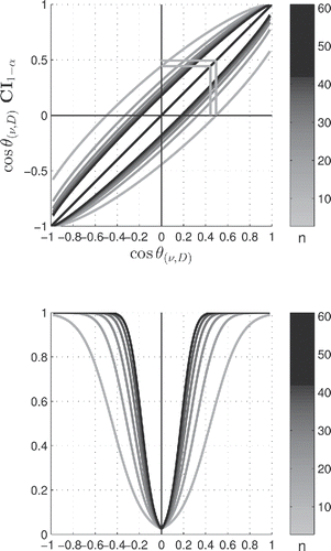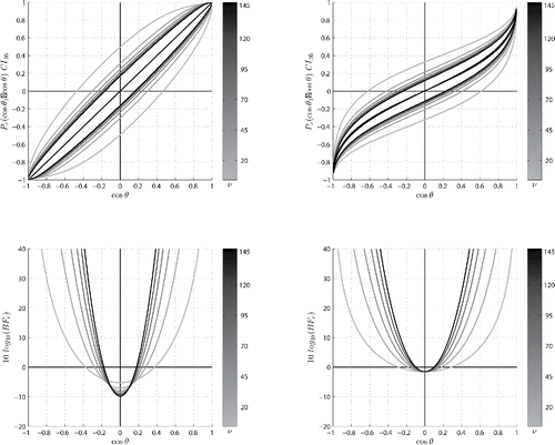10) which simplifies to the expected ± cos θ_α/2 when cos θ_{(ν, D)} = 0. This confidence interval is verified to concur with the usual noncentral t-distribution effect size confidence interval definition (Cumming and Finch 2001). We have plotted in the upper panel of Figure 4 the frequentist two-tail confidence interval cos θ_{(ν, D)} CI_{1 − α} for the continuum of estimates cos θ_{(ν, D)} at confidence level α = .05 and for various two-sample equal size n₁ = n₂ = n. Note that the null hypothesis H_o neatly stands on the vertical line at cos θ = 0. The lower panel in the same figure provides the corresponding statistical test sensitivity (power). It can be readily verified that lower bound of the confidence interval for cos θ_{(ν, D)} is still negative when the latter reaches the critical angle cos θ_α/2. Thus, when applied to the central and noncentral h-distributions, the Neyman–Pearson prescription fails to produce a significant confidence interval at the critical p-value. In fact, Equation (10(10) $$\begin{array}{ccc}\hfill cos{\theta }_{(\nu ,D)}{\text{CI}}_{1-\alpha }& =& {sin}^2{\theta }_{\alpha /2}cos{\theta }_{(\nu ,D)}\hfill \\ & & \pm cos{\theta }_{\alpha /2}\sqrt{1-{sin}^2{\theta }_{\alpha /2}{cos}^2{\theta }_{(\nu ,D)}},\hfill \end{array}$$(10) ) indicates that such a significant confidence interval is achieved at a greater estimate $cos{\theta }_{(\nu ,D)}=cot{\theta }_{\alpha /2}>cos{\theta }_{\alpha /2}$—or, equivalently, lesser $p\text{-}$value—again as illustrated in Figure 4. Now recall that, at confidence level α, the frequentist confidence interval ${\text{CI}}_{1-\alpha }$ is defined such that, on repeated samplings, 1 − α such intervals are expected to contain the true population parameter cos θ_{(ν, Δ)}. For an experiment that barely crosses the significance threshold, the estimates on repeat samplings will fall on either side of the threshold, with $p\text{-}$values and confidence intervals declared significant or not, accordingly. When subjected to such statistical fluctuations, statistical significance thus becomes a “fickle” notion (Nuzzo 2014; Colquhoun 2014; Burnham and Anderson 2014; Halsey et al. 2015; Wasserstein and Lazar 2016).

Figure 3. Null hypothesis significance testing. Type I error at level α and power 1 − β for type II error at level β are represented as intercepts of the cumulative distribution functions of the central and noncentral h-distributions with the critical line at cos θ_α, respectively. Abbreviations: (n)chpdf — (non)central hypersphere probability distribution function; (n)chcdf — (non)central hypersphere cumulative distribution function.

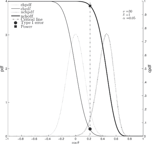
Figure 4. Two-tail frequentist confidence intervals at α = .05 for the continuum of two-sample, equal size n₁ = n₂ = n, cos θ_{(ν, D)} estimates are plotted in the upper panel. The null hypothesis H_o neatly stands on the vertical line at cos θ_{(ν, D)} = 0, from which one can draw critical values horizontally to the diagonal first and vertically to the horizontal polar axis thereafter. The frequentist CI lower bound is still negative when the estimate cos θ_{(ν, D)} reaches the critical angle cos θ_α/2, as exemplified by the inner wedge. The Neyman–Pearson prescription thus fails to produce a significant confidence interval at the critical p-value when applied to the central and noncentral h-distributions. The CI lower bound crosses the zero threshold upward at a larger estimate $cos{\theta }_{(\nu ,D)}=cot{\theta }_{\alpha /2}>cos{\theta }_{\alpha /2}$—or, equivalently, lesser $p\text{-}$value—as exemplified by the outer wedge. For an experiment that barely crosses the significance threshold, the estimates on repeat samplings will fall on either side of the threshold, with $p\text{-}$values and confidence intervals declared significant or not, accordingly. When subjected to such statistical fluctuations, statistical significance thus becomes a “fickle” notion. Lower panel: corresponding power curves.

4. Bayesian Hypothesis Testing Framework

In this section, the Bayesian hypothesis testing framework will be applied to the noncentral h-distribution (7(7) $${\rho }_{(\nu ,\delta )}^h\left(\theta \right)={\mathcal{L}}_{(\nu ,\delta )}^h\left(\theta \right){\rho }_{(\nu ,0)}\left(\theta \right),$$(7) ) considered as a δ-parameterized continuum of hypotheses H₁, with the noncentral parameter δ re-expressed in geometric terms in equation (4(4) $$cos{\theta }_{(\nu ,\delta )}=\frac{\delta /\sqrt{\nu }}{\sqrt{{(\delta /\sqrt{\nu })}^2+1}}=\frac{\delta }{\sqrt{{\delta }^2+\nu }}$$(4) ). The Fisher–Student’s central h-distribution (3(3) $${\rho }_{(\nu ,0)}\left(\theta \right)=\frac{\Gamma \left(\frac{\nu +1}{2}\right)}{\Gamma \left(\frac{1}{2}\right)\Gamma \left(\frac{\nu }{2}\right)}{sin}^{\nu -1}\theta ,0\le \theta \le \pi ,$$(3) ) will considered as H₀. In a Bayesian model selection framework, one is interested in the Bayes factor defined as the ratio of conditional probabilities (11) $$\text{BF}=\frac{P\left(\mathcal{D}\right|H_1)}{P\left(\mathcal{D}\right|H_0)},$$(11) where $\mathcal{D}$ is the data observed. Since the central distribution (3(3) $${\rho }_{(\nu ,0)}\left(\theta \right)=\frac{\Gamma \left(\frac{\nu +1}{2}\right)}{\Gamma \left(\frac{1}{2}\right)\Gamma \left(\frac{\nu }{2}\right)}{sin}^{\nu -1}\theta ,0\le \theta \le \pi ,$$(3) ) is easily factored out of the analytical expression for the noncentral hypersphere distribution (7(7) $${\rho }_{(\nu ,\delta )}^h\left(\theta \right)={\mathcal{L}}_{(\nu ,\delta )}^h\left(\theta \right){\rho }_{(\nu ,0)}\left(\theta \right),$$(7) ), the Bayes factor of interest can be (numerically) computed via the integral (12) $$\begin{array}{ccc}\hfill {\mathrm{BF}}_{\nu }\left(\theta \right)& =& {\int }_0^{\pi }{\mathcal{L}}_{(\nu ,\sqrt{\nu }cot{\theta }_1)}^h\left(\theta \right){\mathrm{Pr}}_{\nu }\left({\theta }_1\right)d{\theta }_1\hfill \\ \hfill & =& {\int }_0^{\pi }\frac{1-cos{\theta }_{1}cos\theta }{{[1-2cos{\theta }_{1}cos\theta +{cos}^2{\theta }_1]}^{\frac{\nu +1}{2}}}{\mathrm{Pr}}_{\nu }\left({\theta }_1\right)d{\theta }_1,\hfill \end{array}$$(12) in terms of the likelihood ratio ${\mathcal{L}}_{(\nu ,\sqrt{\nu }cot{\theta }_1)}^h\left(\theta \right)$ defined in (8(8) $${\mathcal{L}}_{(\nu ,\delta )}^h\left(\theta \right)=\frac{1-cos\theta cos{\theta }_{(\nu ,\delta )}}{{[1-2cos\theta cos{\theta }_{(\nu ,\delta )}+{cos}^2{\theta }_{(\nu ,\delta )}]}^{\frac{\nu +1}{2}}}.$$(8) ) and of a prior Pr_ν(θ₁) to be specified. The relevant posterior probability will then be given by (13) $$P_{\nu }(cos{\theta }_1|cos\theta )={\text{BF}}_{\nu }^{-1}\left(\theta \right){\mathcal{L}}_{(\nu ,\sqrt{\nu }cot{\theta }_1)}^h\left(\theta \right){\mathrm{Pr}}_{\nu }\left({\theta }_1\right).$$(13) It has been abundantly argued in the literature that the choice of prior can have a definitive influence on the Bayes factors and posterior probabilities. Instead of debating the relative merits of various kind of priors, we shall restrain our attention to the following two priors: (1) the proper geometry-naive uniform prior Pr_ν(θ₁) = 1 which should reproduce results stemming from the frequentist framework, and (2) the proper maximal entropy (maxent) prior Pr_ν(θ₁) = ρ_{(ν, 0)}(θ₁) specified by the Fisher–Student’s central h-distribution (3(3) $${\rho }_{(\nu ,0)}\left(\theta \right)=\frac{\Gamma \left(\frac{\nu +1}{2}\right)}{\Gamma \left(\frac{1}{2}\right)\Gamma \left(\frac{\nu }{2}\right)}{sin}^{\nu -1}\theta ,0\le \theta \le \pi ,$$(3) ) itself (Jaynes 1968). The latter choice of maxent prior naturally arises in the present geometrical setting as it meaningfully apportions most of the weight of evidence for H₁ on the equatorial band of a high-dimensional hypersphere where lies the bulk of its density. The latter observation is most pertinent for the biomedical research realm in which “empirical evidence suggests that most medical intervention effects are small or modest” (Pereira, Horwitz, and Ioannidis 2012). This maxent prior avoids Bartlett’s and the information paradoxes (Wang and Liu 2016). The equal-tail Bayesian credible interval ${\text{CI}}_{1-\alpha }$ for the posteriors is given by the integration limits for the integrand (13(13) $$P_{\nu }(cos{\theta }_1|cos\theta )={\text{BF}}_{\nu }^{-1}\left(\theta \right){\mathcal{L}}_{(\nu ,\sqrt{\nu }cot{\theta }_1)}^h\left(\theta \right){\mathrm{Pr}}_{\nu }\left({\theta }_1\right).$$(13) ) which leave out α/2 of the integrand on each tail. We have plotted in the upper panels of Figure 5 the posteriors P_ν(cos θ₁|cos θ) credible intervals for both priors. As expected, the credible interval for the geometry-naive uniform prior recapitulates the results of the frequentist framework: the credible interval straddles the diagonal without correction to the parameter estimate. More interesting is the effect of the maxent prior (3(3) $${\rho }_{(\nu ,0)}\left(\theta \right)=\frac{\Gamma \left(\frac{\nu +1}{2}\right)}{\Gamma \left(\frac{1}{2}\right)\Gamma \left(\frac{\nu }{2}\right)}{sin}^{\nu -1}\theta ,0\le \theta \le \pi ,$$(3) ) which conservatively brings down the Bayesian credible interval below the diagonal. Although the Bayesian statistical hypothesis testing framework is not supposed to be discussed in terms of thresholds, it is interesting to note that the lower bounds of the Bayesian credible intervals in the positive upper quadrants of the upper panels cross the zero threshold upward when the Bayes factor reaches about two and six decibans in the left and right lower panels, at which level the Bayesian evidence is declared barely worth mentioning and substantial, respectively, according to Jeffreys (1998). Finally, recall that the Bayesian credible interval CI_{1 − α} for the parameter cos θ₁ is defined such that, given the observed data, there is 1 − α chance that the true parameter lies in it.

Figure 5. Left panels: geometry-naive uniform prior. Right panels: central hypersphere maxent prior. Upper panels: Bayesian credible intervals CI_0.95 for the posterior P_ν(cos θ₁|cos θ), together with their 0.5 quantiles. Lower panels: corresponding Bayes factors in decibans. The number of degrees of freedom or, equivalently, the hypersphere dimension ν can be deduced from the grayscale colorbars. The Bayesian credible intervals for the geometry-naive uniform prior recapitulate results of the frequentist framework. The central hypersphere maxent prior conservatively brings down the Bayesian credible intervals below the diagonal. Note that the lower bounds of the Bayesian credible intervals in the positive upper quadrants of the upper panels cross the zero threshold upward when the Bayes factor reaches about two and six decibans in the left and right lower panels, at which level the Bayesian evidence is declared barely worth mentioning and substantial, respectively.

5. Applications

When discussing Bayesian analyses in this section, it shall be understood that the analyses will pertain solely to the maxent prior Pr_ν(θ₁) = ρ_{(ν, 0)}(θ₁) specified by the Fisher–Student’s central h-distribution (3(3) $${\rho }_{(\nu ,0)}\left(\theta \right)=\frac{\Gamma \left(\frac{\nu +1}{2}\right)}{\Gamma \left(\frac{1}{2}\right)\Gamma \left(\frac{\nu }{2}\right)}{sin}^{\nu -1}\theta ,0\le \theta \le \pi ,$$(3) ).

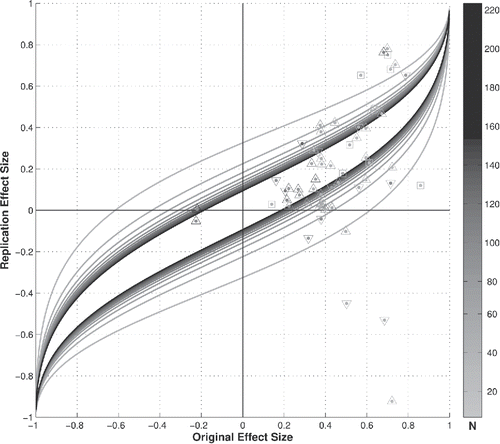
The Open Science Collaboration project (Collaboration et al. 2015) estimated the reproducibility of psychological science to be weak: only 36% of 100 replication attempts produced statistically significant results in terms of the Neyman–Pearson NHST framework p-values, and only 47% of the original effect sizes were within the frequentist CI_0.95 confidence interval of the replication effect size. Etz and Vandekerckhove (2016) argued that the failure of the Reproducibility Project could be attributed to overestimation of the original effect sizes and weak Bayesian evidence in the original studies. Considering the same 72 univariate test-based studies retained by Etz and Vandekerckhove (2016), using the inferential t-statistics they provided in their Supporting Information, and further filtering down—for graphical purposes—to the 60 studies with sample size N less than 220, we have plotted in Figure 6 their original and replication empirical effect sizes against the posteriors’ Bayesian credible intervals. As the posteriors’ Bayesian credible intervals lay under the frequentist diagonal, a now very substantial 75% of the replication effect sizes fall within their respective original effect size posteriors’ credible intervals, indicating that the replication effort was not a failure from a Bayesian perspective. But since 60% of the original credible intervals’ lower bound are found to be negative, it has to be concluded that there was weak Bayesian evidence for the effect sizes in the original studies, in full accord with the conclusions of Etz and Vandekerckhove (2016). Figure 6 shows thus a graphical illustration of the strength of the Bayesian framework: the central h-distribution maxent prior effects an appropriate weighing down of original overestimated effect sizes. In that respect, Ioannidis (2008) has argued that “if priors assume that small effects are plausible but large effects are implausible, Bayes Factors become most promising for small effects,” which is indeed the case here.

Figure 6. The Open Science Collaboration Project original and replication effect sizes plotted against the posteriors’ ${\text{CI}}_{0.95}$ Bayesian credible intervals. Since 75% of the replication effect sizes fall within their original posteriors’ credible intervals, the replication project cannot be called a failure from a Bayesian perspective. Nevertheless, 60% of the original credible intervals’ lower bounds are found to be negative, indicating weak Bayesian evidence for the original effects. The sample sizes can be deduced from the grayscale colorbar: the dot color refer to the initial sample size; an upward (downward) pointing triangle indicates that the replication sample size was bigger (smaller) than the original sample size, while a square indicates that the replication and original sample sizes were identical.

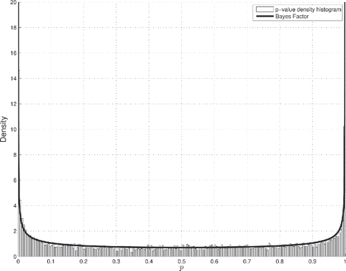
The microarray technology allows for interrogation of the cellular expression of thousands of genes (Schulze and Downward 2001). For illustrative purposes, we have: accessed the NCBI Gene Expression Omnibus head and neck squamous cell carcinoma dataset GSE6631 (Kuriakose et al. 2007b) produced by Kuriakose et al. (2004a) and pertaining to 22 paired samples of normal versus cancerous tissue; extracted the gene probe signals using the Robust Multiarray Analysis (RMA) algorithm (Irizarry et al. 2003); and, finally, filtered out 10% of weakly expressed genes with lowest variances. In Figure 7, the Bayes factor ${\text{BF}}_{\nu =42}\left(p\right)$—defined by Equation (12(12) $$\begin{array}{ccc}\hfill {\mathrm{BF}}_{\nu }\left(\theta \right)& =& {\int }_0^{\pi }{\mathcal{L}}_{(\nu ,\sqrt{\nu }cot{\theta }_1)}^h\left(\theta \right){\mathrm{Pr}}_{\nu }\left({\theta }_1\right)d{\theta }_1\hfill \\ \hfill & =& {\int }_0^{\pi }\frac{1-cos{\theta }_{1}cos\theta }{{[1-2cos{\theta }_{1}cos\theta +{cos}^2{\theta }_1]}^{\frac{\nu +1}{2}}}{\mathrm{Pr}}_{\nu }\left({\theta }_1\right)d{\theta }_1,\hfill \end{array}$$(12) ) but reparameterized in terms of p(θ) as provided by Equation (40(40) $$p\left(\theta \right)=\frac{1}{2}-\frac{cos\theta }{2}\left(1+\frac{1}{2}{sin}^2\theta +\cdots +\frac{1·3·\cdots ·({\nu }_2-3)}{2·4·\cdots ·({\nu }_2-2)}{sin}^{{\nu }_2-2}\theta \right),$$(40) ) in Appendix D—is plotted against the empirical p-value density histogram for 11,302 gene differential expression t-tests. It is seen that the Bayes factor fits extremely well the empirical p-value density, both in the middle of the graph where Bayesian evidence favors H_o, and at critical p-values at both ends of the range where Bayesian evidence favors H₁. Recall that the Fisher–Student’s central h-distribution p-value density is the uniform density U(0, 1) on the range 0 ⩽ p ⩽ 1, a restatement of the probability transform theorem which stipulates that the distribution of p-values under the null hypothesis is uniform. On this p-range, the Bayes factor defined in Equation (11(11) $$\text{BF}=\frac{P\left(\mathcal{D}\right|H_1)}{P\left(\mathcal{D}\right|H_0)},$$(11) ) simply reads $\mathrm{BF}=P\left(\mathcal{D}\right|H_1),$ as the denominator simplifies to $P\left(\mathcal{D}\right|H_o)=1.$ More precisely, we prove in Appendix E that the Bayes factor BF_ν(p) is a bona fide probability distribution, modeling the H₁-associated nonuniform p-value density in lieu of the H_o-associated uniform p-value density U(0, 1).

Figure 7. Bayes factor ${\text{BF}}_{\nu }\left(p\right)$ against a microarray empirical p-value density histogram. The Bayes factor ${\text{BF}}_{\nu =42}\left(p\right)$ is plotted against the p-value density histogram for 11,302 gene differential expression t-tests of the GEO dataset with accession number GSE6631. On the range 0 ⩽ p ⩽ 1, the Fisher–Student’s central h-distribution p-value density simplifies to the uniform density U(0, 1). On this range, the Bayes factor therefore simply reads $\mathrm{BF}=P\left(\mathcal{D}\right|H_1)/P\left(\mathcal{D}\right|H_0)=P\left(\mathcal{D}\right|H_1).$ The Bayes factor fits extremely well the empirical p-value density, both in the middle of the graph where Bayesian evidence favors H_o, and at critical p-values where Bayesian evidence favors H₁.

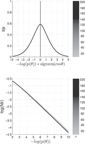
Since the microarray technology simultaneously interrogates the cellular expression of thousands of genes, one is readily confronted with the multiple hypothesis testing problem within the frequentist NHST framework (Dudoit, Shaffer, and Boldrick 2003). Efron (2008) proposed a local false discovery rate (fdr) in terms of a two-group mixture density model of “null genes” and “nonnull genes” to address this problem. The present Bayesian approach affords a very economical definition of a local fdr in terms of the Bayes factor BF_ν(p):(14) $$\text{fdr}\left(p\right)=\frac{P\left(\mathcal{D}\right|H_o)}{P\left(\mathcal{D}\right|H_o)+P\left(\mathcal{D}\right|H_1)}=\frac{1}{1+{\mathrm{BF}}_{\nu }\left(p\right)}.$$(14) We have, in the upper panel of Figure 8 plotted the local fdr on a p-value log-scale, while the lower panel can be used to assess the local fdr for vanishing p-values on a log-log scale. It is interesting to note that the curves for the local fdr are independent of the corresponding hypersphere number of degrees of

 

freedom ν and are essentially linear on a log–log scale in the relevant subdomain of vanishing $p\text{-}$values, a fact which attributes a degree of universality to the present Bayesian hypothesis testing framework based on the noncentral h-distribution (7(7) $${\rho }_{(\nu ,\delta )}^h\left(\theta \right)={\mathcal{L}}_{(\nu ,\delta )}^h\left(\theta \right){\rho }_{(\nu ,0)}\left(\theta \right),$$(7) ) with the central Fisher–Student’s h-distribution (3(3) $${\rho }_{(\nu ,0)}\left(\theta \right)=\frac{\Gamma \left(\frac{\nu +1}{2}\right)}{\Gamma \left(\frac{1}{2}\right)\Gamma \left(\frac{\nu }{2}\right)}{sin}^{\nu -1}\theta ,0\le \theta \le \pi ,$$(3) ) as geometrically meaningful maxent prior.

Figure 8. Local false discovery rate $1/(1+{\text{BF}}_{\nu }\left(p\right))$ in terms of the Bayes factor ${\text{BF}}_{\nu }\left(p\left(\theta \right)\right),$ where ν is the hypersphere dimension which can be deduced from the grayscale colorbar. Upper panel: two-tail local fdr. Note the signed log-scale on the horizontal axis. Lower panel: blow-up and extension of the right-hand tail of the upper panel on a log–log scale. The local fdr curves are independent of the hypersphere number of degrees of freedom ν and are essentially linear on a log–log scale in the subdomain covered in the latter panel, a fact which attributes a degree of universality to the Bayesian hypothesis testing framework based on the noncentral h-distribution, with the central Fisher–Student’s h-distribution as geometrically meaningful maxent prior.

6. Conclusion

Using simple geometric concepts such as vectors, matrix projectors and trigonometric quantities, we have derived an analytical noncentral extension to the Fisher–Student’s central hypersphere distribution. Characterized by the single noncentrality parameter δ, this analytical noncentral h-distribution has allowed us to graphically assess the limitations of the Neyman–Pearson null hypothesis significance testing framework and the strengths of the Bayesian hypothesis analysis framework on a nontrivial one-dimensional compact parametric space. The central Fisher–Student’s hypersphere h-distribution has been geometrically argued to be an appropriate maxent prior. The corresponding Bayes factor and posteriors have been demonstrated to remedy in part to the vexing question of the reproducibility of science, by modulating down overestimated size effects that a frequentist analysis would inevitably produce. The Bayes factor has been shown to adequately model the empirical p-value density of a multiple hypothesis testing dataset produced by the microarray technology, and to provide easy assessment of a local false discovery rate. The noncentral h-distribution has thus allowed us to address all the intricacies of both the Neyman–Pearson null hypothesis significance testing framework and the Bayesian hypothesis analysis framework while avoiding use of the unwieldy noncentral t-distribution or problems arising from working in higher-dimensional parametric spaces. As such, the noncentral hypersphere h-distribution has relevance both as a practical tool and as a pedagogical tool for a broad audience.

 

A. Projector Matrices

The N × N matrix projectors P_C, P_B and P_W, which respectively project the observation N-vector o on the overall center-of-mass, the between-class variance hyperplane and the within-class variance hyperplane, are given by the matrices (15) $$\begin{array}{ccc}\hfill P_C& =& \frac{1}{N}{\left(\mathbf{1}{\mathbf{1}}^t\right)}_{N\times N},\hfill \\ \hfill \\ \hfill P_B& =& \left(\begin{array}{cccc}\hfill \frac{1}{n_1}{\left(\mathbf{1}{\mathbf{1}}^t\right)}_{n_1\times n_1}& & & 0\\ & \hfill \frac{1}{n_2}{\left(\mathbf{1}{\mathbf{1}}^t\right)}_{n_2\times n_2}& & \\ & & \hfill \ddots & \\ \hfill 0& & & \frac{1}{n_{{\nu }_1}}{\left(\mathbf{1}{\mathbf{1}}^t\right)}_{n_{{\nu }_1+1}\times n_{{\nu }_1+1}}\end{array}\right)-P_C,\hfill \\ \hfill \\ \hfill P_W& =& \left(\begin{array}{cccc}\hfill I_{n_1}-\frac{1}{n_1}{\left(\mathbf{1}{\mathbf{1}}^t\right)}_{n_1\times n_1}& & & 0\\ & \hfill I_{n_2}-\frac{1}{n_2}{\left(\mathbf{1}{\mathbf{1}}^t\right)}_{n_2\times n_2}& & \\ & & \hfill \ddots & \\ \hfill 0& & & I_{n_{{\nu }_1+1}}-\frac{1}{n_{{\nu }_1+1}}{\left(\mathbf{1}{\mathbf{1}}^t\right)}_{n_{{\nu }_1+1}\times n_{{\nu }_1+1}}\end{array}\right)\hfill \end{array}$$(15) where $[n_1,n_2,\cdots ,n_{{\nu }_1+1}]$ partitions the total of N = ∑^{ν₁ + 1}_{i = 1}n_i observations composing the observation N-vector o into ν₁ + 1 respective class cardinalities. The projectors obey the identity resolution (16) $$I_N=P_C+P_B+P_W,$$(16) with I_N the identity matrix. Recall that a matrix projector obeys the defining property P² = P, with eigenvalue equation λ(λ − 1) = 0: its eigenvalues are thus restricted to the values {0, 1}, and its rank is provided by the cardinality of the set of its non-vanishing unit eigenvalues. The projectors P_C, P_B and P_W have ranks 1, ν₁ and ν₂ = N − ν₁ − 1, respectively. The two-sample case corresponds to ν₁ = 1.

B. Determination of the Sampling Distribution

Using the matrix resolution of the identity (16(16) $$I_N=P_C+P_B+P_W,$$(16) ), consider the situation when the within-class uniform centered vector (17) $$\begin{array}{ccc}\hfill \left(I_N-P_C\right)\left(\begin{array}{c}{\delta }_1{\mathbf{1}}_{n_1}\\ {\delta }_2{\mathbf{1}}_{n_2}\end{array}\right)& =& (P_B+P_W)\left(\begin{array}{c}{\delta }_1{\mathbf{1}}_{n_1}\\ {\delta }_2{\mathbf{1}}_{n_2}\end{array}\right)=P_B\left(\begin{array}{c}{\delta }_1{\mathbf{1}}_{n_1}\\ {\delta }_2{\mathbf{1}}_{n_2}\end{array}\right)\hfill \\ & =& {\mathbf{T}}_B{\mathbf{T}}_B^t\left(\begin{array}{c}{\delta }_1{\mathbf{1}}_{n_1}\\ {\delta }_2{\mathbf{1}}_{n_2}\end{array}\right)=\frac{{\delta }_1-{\delta }_2}{\sqrt{\frac{1}{n_1}+\frac{1}{n_2}}}{\mathbf{T}}_B\hfill \end{array}$$(17) along the unit polar axis T_B is added to an observation vector drawn from a population with null noncentrality parameter. In the two group comparison context, this will impart the nonvanishing normalized effect size δ₁ to the first subpopulation, and the nonvanishing normalized effect size δ₂ to the second subpopulation. Under these circumstances, the two-sample t-statistic (1(1) $$\begin{array}{ccc}\hfill t& =& {\left[\nu \frac{{\mathbf{o}}^t{P}_B\mathbf{o}}{{\mathbf{o}}^t{P}_W\mathbf{o}}\right]}^{1/2}=\sqrt{\nu }\frac{cos\theta }{sin\theta },\hfill \\ & & -\infty \le t\le \infty ,0\le \theta \le \pi ,\nu =N-2.\hfill \end{array}$$(1) ) will distribute according to the noncentral h-distribution ρ_{(ν, Δ)}(θ), with noncentrality parameter Δ given by the factor multiplying T_B above, that is, (18) $$\begin{array}{ccc}\hfill \Delta ={\mathbf{T}}_B^t\left(\begin{array}{c}{\delta }_1{\mathbf{1}}_{n_1}\\ {\delta }_2{\mathbf{1}}_{n_2}\end{array}\right)& =& \frac{\delta }{\sqrt{\frac{1}{n_1}+\frac{1}{n_2}}},\delta ={\delta }_1-{\delta }_2,\hfill \\ & =& \sqrt{\frac{n}{2}}\delta \text{if}{n}_1=n_2=n.\hfill \end{array}$$(18) The quantity (19) $$\begin{array}{ccc}\hfill cot{\theta }_{(\nu ,\Delta )}=\frac{\Delta }{\sqrt{\nu }}& =& \frac{\delta }{\sqrt{\nu \left(\frac{1}{n_1}+\frac{1}{n_2}\right)}}\hfill \\ & =& \sqrt{\frac{n}{n-1}}\frac{\delta }{2}\text{if}{n}_1=n_2=n,\nu =2n-2,\hfill \\ & \simeq & \frac{\delta }{2}\text{for}\text{large}{n}_1=n_2=n\hfill \end{array}$$(19) is needed to determine the noncentrality parameter (20) $$\begin{array}{ccc}\hfill cos{\theta }_{(\nu ,\Delta )}& =& \frac{\Delta /\sqrt{\nu }}{\sqrt{{(\Delta /\sqrt{\nu })}^2+1}}=\frac{\Delta }{\sqrt{{\Delta }^2+\nu }}=\frac{\delta }{\sqrt{{\delta }^2+\nu \left(\frac{1}{n_1}+\frac{1}{n_2}\right)}}\hfill \\ & =& \frac{\delta }{\sqrt{{\delta }^2+4\frac{n-1}{n}}}\text{if}{n}_1=n_2=n,\nu =2n-2,\hfill \\ & \simeq & \frac{\delta }{\sqrt{{\delta }^2+4}}=cos{\theta }_{(\nu ,\sqrt{\nu }\delta /2)}\text{for}\text{large}{n}_1=n_2=n\hfill \end{array}$$(20) as reexpressed in trigonometric terms. We have carried out the latter tedious enumeration of square root factors because they are often introduced summarily in the literature with no reference to their simple geometric origin. See, e.g., Ellis (2010).

C. Noncentral Hypersphere F-distribution

The F-statistic is defined in both projection and geometrical terms via the variance ratio (21) $$F_{({\nu }_1,{\nu }_2)}\left(\theta \right)=\frac{{\nu }_2}{{\nu }_1}\frac{{\mathbf{o}}^t{P}_B\mathbf{o}}{{\mathbf{o}}^t{P}_W\mathbf{o}}=\frac{{\nu }_2}{{\nu }_1}\frac{{cos}^2\theta }{{sin}^2\theta },$$(21) where ν₁ and ν₂ are the dimensions of the between-class and within-class variance hyperplanes, respectively. The matrix projector P_B and P_W are defined in Appendix A. Geometrically, θ is the angle between the observation vector o and the between-class variance hyperplane, and π/2 − θ the angle between o and the orthogonal pooled within-class variance hyperplane. When the observation o has uniform class-independent isotropic distribution on the central unit radius hypersphere ${\mathcal{S}}^{{\nu }_1+{\nu }_2},$ F distributes according to the central (Λ = 0) Fisher–Snedecor F-distribution (22) $${\rho }_{({\nu }_1,{\nu }_2,\Lambda =0)}\left(\theta \right)=2\frac{\Gamma \left(\frac{{\nu }_1+{\nu }_2}{2}\right)}{\Gamma \left(\frac{{\nu }_1}{2}\right)\Gamma \left(\frac{{\nu }_2}{2}\right)}{cos}^{{\nu }_1-1}\theta {sin}^{{\nu }_2-1}\theta ,0\le \theta \le \frac{\pi }{2}.$$(22) The NHST p-value is obtained by computing the probability of having an observation with angular distance θ′ ⩽ θ to the between-class variance hyperplane: it is given by (23) $$p\left(\theta \right)=2\frac{\Gamma \left(\frac{{\nu }_1+{\nu }_2}{2}\right)}{\Gamma \left(\frac{{\nu }_1}{2}\right)\Gamma \left(\frac{{\nu }_2}{2}\right)}{\int }_0^{\theta }{cos}^{{\nu }_1-1}{\theta }^{\text{'}}{sin}^{{\nu }_2-1}{\theta }^{\text{'}}\text{d}{\theta }^{\text{'}},0\le \theta \le \frac{\pi }{2},$$(23) the integration of which can be carried out analytically: see Appendix D. We shall find convenient in the following to effect the change of variable R = cos θ in order to reexpress the central Fisher–Snedecor F-distribution (22(22) $${\rho }_{({\nu }_1,{\nu }_2,\Lambda =0)}\left(\theta \right)=2\frac{\Gamma \left(\frac{{\nu }_1+{\nu }_2}{2}\right)}{\Gamma \left(\frac{{\nu }_1}{2}\right)\Gamma \left(\frac{{\nu }_2}{2}\right)}{cos}^{{\nu }_1-1}\theta {sin}^{{\nu }_2-1}\theta ,0\le \theta \le \frac{\pi }{2}.$$(22) ) as (24) $${\rho }_{({\nu }_1,{\nu }_2,\Lambda =0)}\left(R\right)=2\frac{\Gamma \left(\frac{{\nu }_1+{\nu }_2}{2}\right)}{\Gamma \left(\frac{{\nu }_1}{2}\right)\Gamma \left(\frac{{\nu }_2}{2}\right)}{R}^{{\nu }_1-1}{(1-R^2)}^{\frac{{\nu }_2-2}{2}},0\le R\le 1,$$(24) with R a correlation-like parameter. Consider now the projection of the observation vector o on the between-class variance hyperplane. Since P_B is a projector operator of rank ν₁, it is invariant under rotation within the corresponding unit-eigenvalue eigenspace. This eigenspace degeneracy will allow us to perform the noncentral hypersphere cosine translation (25) $$cos{\theta }_{({\nu }_2,\Lambda )}=\sqrt{\Lambda /(\Lambda +{\nu }_2)}$$(25) expressed in terms of the noncentrality parameter Λ for the noncentral F-distribution along a unit vector ${\mathbf{T}}_{\Lambda }$ of our choosing in this eigenspace. In the coordinate system centered on the hypersphere, we thus define the polar coordinates (26) $$\begin{array}{ccc}\hfill {\mathbf{o}}^t\left({\mathbf{T}}_{\Lambda }{\mathbf{T}}_{\Lambda }^t\right)\mathbf{o}& =& R^2{cos}^2\phi ,\hfill \\ \hfill {\mathbf{o}}^t(P_B-{\mathbf{T}}_{\Lambda }{\mathbf{T}}_{\Lambda }^t)\mathbf{o}& =& R^2{sin}^2\phi .\hfill \end{array}$$(26) The 3-vector $(Rcos\phi ,Rsin\phi ,\sqrt{1-R^2})$ is easily argued to distribute according to the joint distribution (27) $$\begin{array}{ccc}\hfill {\rho }_{({\nu }_1,{\nu }_2,0)}(R,\phi )& =& {\rho }_{({\nu }_1,{\nu }_2,0)}\left(R\right)\times {\rho }_{({\nu }_1-1,0)}\left(\phi \right),0\le R\le 1,0\le \phi \le \pi ,{\nu }_1\ge 2,\hfill \\ & =& 2\frac{\Gamma \left(\frac{{\nu }_1+{\nu }_2}{2}\right)}{\Gamma \left(\frac{{\nu }_1}{2}\right)\Gamma \left(\frac{{\nu }_2}{2}\right)}{R}^{{\nu }_1-1}{(1-R^2)}^{\frac{{\nu }_2-2}{2}}\times \frac{\Gamma \left(\frac{{\nu }_1}{2}\right)}{\Gamma \left(\frac{1}{2}\right)\Gamma \left(\frac{{\nu }_1-1}{2}\right)}{sin}^{{\nu }_1-2}\phi ,\hfill \end{array}$$(27) where ${\rho }_{({\nu }_1-1,0)}\left(\phi \right)$ is the Fisher–Student’s central $t\text{-}$distribution (3(3) $${\rho }_{(\nu ,0)}\left(\theta \right)=\frac{\Gamma \left(\frac{\nu +1}{2}\right)}{\Gamma \left(\frac{1}{2}\right)\Gamma \left(\frac{\nu }{2}\right)}{sin}^{\nu -1}\theta ,0\le \theta \le \pi ,$$(3) ). When the noncentrality parameter Λ is nonvanishing, the observation vector as assessed in the observation coordinate system shall similarly read $(rcos\psi ,rsin\psi ,\sqrt{1-r^2}),$ with its polar coordinates r and ψ both function of the noncentral parameter (25(25) $$cos{\theta }_{({\nu }_2,\Lambda )}=\sqrt{\Lambda /(\Lambda +{\nu }_2)}$$(25) ). Indeed, when the latter 3-vector is recentered on the translated hypersphere and renormalized, it reads (28) $$(rcos\psi ,rsin\psi ,\sqrt{1-r^2})\Rightarrow \frac{\left(rcos\psi -cos{\theta }_{({\nu }_2,\Lambda )},rsin\psi ,\sqrt{1-r^2}\right)}{{[1-2rcos\psi cos{\theta }_{({\nu }_2,\Lambda )}+{cos}^2{\theta }_{({\nu }_2,\Lambda )}]}^{1/2}},$$(28) which leads us to consider the polar coordinate transformation (29) $$R={\left[\frac{r^2-2rcos\psi cos{\theta }_{({\nu }_2,\Lambda )}+{cos}^2{\theta }_{({\nu }_2,\Lambda )}}{1-2rcos\psi cos{\theta }_{({\nu }_2,\Lambda )}+{cos}^2{\theta }_{({\nu }_2,\Lambda )}}\right]}^{1/2}\text{and}\phi =\text{arcot}\left(\frac{rcos\psi -cos{\theta }_{({\nu }_2,\Lambda )}}{rsin\psi }\right).$$(29) The transformation Jacobian is given by (30) $$\begin{array}{ccc}\hfill \phantom{x}{J}_{({\nu }_1,{\nu }_2,\Lambda )}(r,\psi )& =& \frac{\partial (R,\phi )}{\partial (r,\psi )}\hfill \\ & =& \frac{r(1-rcos\psi cos{\theta }_{({\nu }_2,\Lambda )})}{{[r^2-2rcos\psi cos{\theta }_{({\nu }_2,\Lambda )}+{cos}^2{\theta }_{({\nu }_2,\Lambda )}]}^{1/2}{[1-2rcos\psi cos{\theta }_{({\nu }_2,\Lambda )}+{cos}^2{\theta }_{({\nu }_2,\Lambda )}]}^{3/2}},\hfill \end{array}$$(30) where the denominator term $[r^2-2rcos\psi cos{\theta }_{({\nu }_2,\Lambda )}+{cos}^2{\theta }_{({\nu }_2,\Lambda )}]$ is noted to vanish at the center of the translated hypersphere, that is, at $(r,\psi )=(cos{\theta }_{({\nu }_2,\Lambda )},0).$ Introducing the transformation (29(29) $$R={\left[\frac{r^2-2rcos\psi cos{\theta }_{({\nu }_2,\Lambda )}+{cos}^2{\theta }_{({\nu }_2,\Lambda )}}{1-2rcos\psi cos{\theta }_{({\nu }_2,\Lambda )}+{cos}^2{\theta }_{({\nu }_2,\Lambda )}}\right]}^{1/2}\text{and}\phi =\text{arcot}\left(\frac{rcos\psi -cos{\theta }_{({\nu }_2,\Lambda )}}{rsin\psi }\right).$$(29) ) into the joint distribution (27(27) $$\begin{array}{ccc}\hfill {\rho }_{({\nu }_1,{\nu }_2,0)}(R,\phi )& =& {\rho }_{({\nu }_1,{\nu }_2,0)}\left(R\right)\times {\rho }_{({\nu }_1-1,0)}\left(\phi \right),0\le R\le 1,0\le \phi \le \pi ,{\nu }_1\ge 2,\hfill \\ & =& 2\frac{\Gamma \left(\frac{{\nu }_1+{\nu }_2}{2}\right)}{\Gamma \left(\frac{{\nu }_1}{2}\right)\Gamma \left(\frac{{\nu }_2}{2}\right)}{R}^{{\nu }_1-1}{(1-R^2)}^{\frac{{\nu }_2-2}{2}}\times \frac{\Gamma \left(\frac{{\nu }_1}{2}\right)}{\Gamma \left(\frac{1}{2}\right)\Gamma \left(\frac{{\nu }_1-1}{2}\right)}{sin}^{{\nu }_1-2}\phi ,\hfill \end{array}$$(27) ) and regrouping the various terms, we find that (31) $${\rho }_{({\nu }_1,{\nu }_2,\Lambda )}^h(r,\psi )={\mathcal{L}}_{({\nu }_1,{\nu }_2,\Lambda )}^h(r,\psi ){\rho }_{({\nu }_1,{\nu }_2,0)}\left(r\right),{\nu }_1\ge 2,$$(31) where ${\rho }_{({\nu }_1,{\nu }_2,0)}\left(r\right)$ is the central Fisher–Snedecor F-distribution (24(24) $${\rho }_{({\nu }_1,{\nu }_2,\Lambda =0)}\left(R\right)=2\frac{\Gamma \left(\frac{{\nu }_1+{\nu }_2}{2}\right)}{\Gamma \left(\frac{{\nu }_1}{2}\right)\Gamma \left(\frac{{\nu }_2}{2}\right)}{R}^{{\nu }_1-1}{(1-R^2)}^{\frac{{\nu }_2-2}{2}},0\le R\le 1,$$(24) ), and where the likelihood function ${\mathcal{L}}_{({\nu }_1,{\nu }_2,\Lambda )}^h$ is given by (32) $${\mathcal{L}}_{({\nu }_1,{\nu }_2,\Lambda )}^h(r,\psi )=\frac{\Gamma \left(\frac{{\nu }_1}{2}\right)}{\Gamma \left(\frac{1}{2}\right)\Gamma \left(\frac{{\nu }_1-1}{2}\right)}\frac{(1-rcos\psi cos{\theta }_{({\nu }_2,\Lambda )}){sin}^{{\nu }_1-2}\psi }{{[1-2rcos\psi cos{\theta }_{({\nu }_2,\Lambda )}+{cos}^2{\theta }_{({\nu }_2,\Lambda )}]}^{\frac{{\nu }_1+{\nu }_2}{2}}},$$(32) with neat cancelation of all singular terms. When Λ = 0, we have that $cos{\theta }_{({\nu }_2,\Lambda )}=0,$ ψ = ϕ, r = R, and ${\rho }_{({\nu }_1,{\nu }_2,\Lambda )}^h(r,\psi )$ simplifies to the central Fisher–Snedecor $F\text{-}$distribution ${\rho }_{({\nu }_1,{\nu }_2,0)}(R,\phi )$ defined by equation (27(27) $$\begin{array}{ccc}\hfill {\rho }_{({\nu }_1,{\nu }_2,0)}(R,\phi )& =& {\rho }_{({\nu }_1,{\nu }_2,0)}\left(R\right)\times {\rho }_{({\nu }_1-1,0)}\left(\phi \right),0\le R\le 1,0\le \phi \le \pi ,{\nu }_1\ge 2,\hfill \\ & =& 2\frac{\Gamma \left(\frac{{\nu }_1+{\nu }_2}{2}\right)}{\Gamma \left(\frac{{\nu }_1}{2}\right)\Gamma \left(\frac{{\nu }_2}{2}\right)}{R}^{{\nu }_1-1}{(1-R^2)}^{\frac{{\nu }_2-2}{2}}\times \frac{\Gamma \left(\frac{{\nu }_1}{2}\right)}{\Gamma \left(\frac{1}{2}\right)\Gamma \left(\frac{{\nu }_1-1}{2}\right)}{sin}^{{\nu }_1-2}\phi ,\hfill \end{array}$$(27) ). 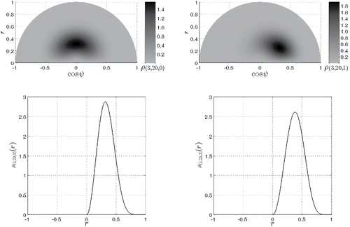The density ${\rho }_{({\nu }_1,{\nu }_2,\Lambda )}^h(r,\psi )$ can be drawn on a two-dimensional half-circle as in Figure 9, with the polar coordinates (r, ψ) summarizing the between-class variance hyperplane coordinates. We are ultimately interested in the distribution of $F_{({\nu }_1,{\nu }_2,\Lambda )}\left(r\right)$ parameterized by the correlation-like parameter r only. The desired distribution function is obtained by computing the marginal distribution of (31(31) $${\rho }_{({\nu }_1,{\nu }_2,\Lambda )}^h(r,\psi )={\mathcal{L}}_{({\nu }_1,{\nu }_2,\Lambda )}^h(r,\psi ){\rho }_{({\nu }_1,{\nu }_2,0)}\left(r\right),{\nu }_1\ge 2,$$(31) ), that is, by integrating it with respect to polar coordinate angle ψ, as is graphically illustrated in Figure 9. We thus have that $F_{({\nu }_1,{\nu }_2,\Lambda )}\left(r\right)$ distributes according to (33) $${\rho }_{({\nu }_1,{\nu }_2,\Lambda )}^h\left(r\right)={\mathcal{L}}_{({\nu }_1,{\nu }_2,\Lambda )}^h\left(r\right){\rho }_{({\nu }_1,{\nu }_2,0)}\left(r\right),{\nu }_1\ge 2,$$(33) with (34) $${\mathcal{L}}_{({\nu }_1,{\nu }_2,\Lambda )}^h\left(r\right)={\int }_{\psi =0}^{\pi }{\mathcal{L}}_{({\nu }_1,{\nu }_2,\Lambda )}^h(r,\psi )\text{d}\psi .$$(34)

Figure 9. Left upper panel: central Fisher–Snedecor F-distribution ${\rho }_{({\nu }_1=3,{\nu }_2=20,\Lambda =0)}(r,\psi )$ plotted on the between-class variance hyperplane summarized by the polar coordinates (r, ψ). Right upper panel: noncentral h-distribution ${\rho }_{({\nu }_1=3,{\nu }_2=20,\Lambda =1)}^h(r,\psi )$ similarly plotted on the between-class variance hyperplane. Left lower panel: central Fisher–Snedecor F-distribution ${\rho }_{({\nu }_1=3,{\nu }_2=20,\Lambda =0)}\left(r\right)$ as plotted along the correlation-like r axis: it is the marginal distribution of the distribution above it, graphically obtained by circularly sweeping the distribution radar-like from ψ = −π to ψ = 0 and projecting the sweep result on the positive axis of the lower panel. Right lower panel: noncentral h-distribution ${\rho }_{({\nu }_1=3,{\nu }_2=20,\Lambda =1)}^h\left(r\right)$ as plotted along the correlation-like r axis: again, it is the marginal distribution of the distribution above it.

The special case ν₁ = 1 is given by (35) $${\rho }_{({\nu }_1=1,{\nu }_2,\Lambda )}^h\left(r\right)=\sum _{r^{\text{'}}=\{r,-r\}}{\rho }_{({\nu }_2,\Lambda )}^h\left(r^{\text{'}}\right),$$(35) where ${\rho }_{({\nu }_2,\Lambda )}^h\left(r\right)$ is the noncentral h-distribution (7(7) $${\rho }_{(\nu ,\delta )}^h\left(\theta \right)={\mathcal{L}}_{(\nu ,\delta )}^h\left(\theta \right){\rho }_{(\nu ,0)}\left(\theta \right),$$(7) ) reexpressed in terms of the correlation-like r parameter: (36) $${\rho }_{({\nu }_2,\Lambda )}^h\left(r\right)=\frac{\Gamma \left(\frac{{\nu }_2+1}{2}\right)}{\Gamma \left(\frac{1}{2}\right)\Gamma \left(\frac{{\nu }_2}{2}\right)}\frac{(1-rcos{\theta }_{({\nu }_2,\Lambda )}){(1-r^2)}^{\frac{{\nu }_2-2}{2}}}{{[1-2rcos{\theta }_{({\nu }_2,\Lambda )}+{cos}^2{\theta }_{({\nu }_2,\Lambda )}]}^{\frac{{\nu }_2+1}{2}}}.$$(36) For the sake of comparison, we state without proof that the noncentral F-distribution can be expressed as (37) $${\rho }_{({\nu }_1,{\nu }_2,\Lambda )}^F\left(r\right)={\mathcal{L}}_{({\nu }_1,{\nu }_2,\Lambda )}^F\left(r\right){\rho }_{({\nu }_1,{\nu }_2,0)}\left(r\right),$$(37) with the likelihood function ${\mathcal{L}}_{({\nu }_1,{\nu }_2,\Lambda )}^F\left(r\right)$ defined by the cumbersome infinite sum of terms (Walck (2007)) $${\mathcal{L}}_{({\nu }_1,{\nu }_2,\Lambda )}^F\left(r\right)=e^{-\frac{\Lambda }{2}}\sum _{j=0}^{\infty }\frac{1}{j!}{\left(\frac{\Lambda }{2}\right)}^j\frac{\Gamma \left(\frac{{\nu }_1+{\nu }_2+2j}{2}\right)}{\Gamma \left(\frac{{\nu }_1+{\nu }_2}{2}\right)}\frac{\Gamma \left(\frac{{\nu }_1}{2}\right)}{\Gamma \left(\frac{{\nu }_1+2j}{2}\right)}{r}^{2j}.$$Equations (33(33) $${\rho }_{({\nu }_1,{\nu }_2,\Lambda )}^h\left(r\right)={\mathcal{L}}_{({\nu }_1,{\nu }_2,\Lambda )}^h\left(r\right){\rho }_{({\nu }_1,{\nu }_2,0)}\left(r\right),{\nu }_1\ge 2,$$(33) ) and (37(37) $${\rho }_{({\nu }_1,{\nu }_2,\Lambda )}^F\left(r\right)={\mathcal{L}}_{({\nu }_1,{\nu }_2,\Lambda )}^F\left(r\right){\rho }_{({\nu }_1,{\nu }_2,0)}\left(r\right),$$(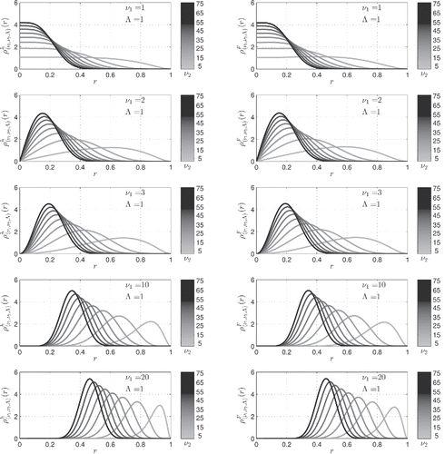37) ) are graphically compared in Figure 10. The latter distribution is known to generate numerical instabilities. Indeed, Baharev, Schichl, and Rév (2017) state that “computations involving the noncentral F-distribution are notoriously difficult to implement properly in floating-point arithmetic: catastrophic loss of precision, floating-point underflow and overflow, drastically increasing computation time and program hang-ups, and instability due to numerical cancellation have all been reported.” The simpler analytical expression (33(33) $${\rho }_{({\nu }_1,{\nu }_2,\Lambda )}^h\left(r\right)={\mathcal{L}}_{({\nu }_1,{\nu }_2,\Lambda )}^h\left(r\right){\rho }_{({\nu }_1,{\nu }_2,0)}\left(r\right),{\nu }_1\ge 2,$$(33) ) for the noncentral hypersphere distribution should help avoiding such numerical instabilities, while allowing easier exploitation of the Bayesian hypothesis testing framework as was carried out in Section 4. Finally, note that definitions of the noncentrality parameter Λ vary in the literature: numerical computations as carried in Figure 10 indicates that equation (25(25) $$cos{\theta }_{({\nu }_2,\Lambda )}=\sqrt{\Lambda /(\Lambda +{\nu }_2)}$$(25) ) refers to the parameter λ (herein Λ) used by Walck (2007).

Figure 10. Left panels: probability density curves for the noncentral hypersphere distribution ${\rho }_{({\nu }_1,{\nu }_2,\Lambda )}^h\left(r\right),$ for the parameters (Λ, ν₁) stated in the legend and ν₂ which can be deduced from the grayscale colorbar. Right panels: probability density curves for the noncentral F-distribution ${\rho }_{({\nu }_1,{\nu }_2,\Lambda )}^F\left(r\right)$ for the same parameter set. The noncentral hypersphere distribution ${\rho }_{({\nu }_1,{\nu }_2,\Lambda )}^h\left(r\right)$ offers a very economical analytic alternative to the noncentral F-distribution ${\rho }_{({\nu }_1,{\nu }_2,\Lambda )}^F\left(r\right).$

D. Analytic Expressions for the Cumulative Distribution Functions (p-values)

Cumulative distribution functions, thus p-values, (38) $$p\left(\theta \right)=\frac{\Gamma \left(\frac{{\nu }_2+1}{2}\right)}{\Gamma \left(\frac{1}{2}\right)\Gamma \left(\frac{{\nu }_2}{2}\right)}{\int }_0^{\theta }{sin}^{{\nu }_2-1}\theta d\theta ,0\le \theta \le \pi ,$$(38) for the central Fisher–Student t-distribution (3(3) $${\rho }_{(\nu ,0)}\left(\theta \right)=\frac{\Gamma \left(\frac{\nu +1}{2}\right)}{\Gamma \left(\frac{1}{2}\right)\Gamma \left(\frac{\nu }{2}\right)}{sin}^{\nu -1}\theta ,0\le \theta \le \pi ,$$(3) ) can be computed analytically in trigonometric terms. One finds for ν₂ odd (39) $$p\left(\theta \right)=\frac{\theta }{\pi }-\frac{sin\theta cos\theta }{\pi }\left(1+\frac{2}{3}{sin}^2\theta +\cdots +\frac{2·4·\cdots ·({\nu }_2-3)}{3·5·\cdots ·({\nu }_2-2)}{sin}^{{\nu }_2-3}{\theta }_y\right),$$(39) where only the first term should be retained for ν₂ = 1, the first two terms for ν₂ = 3, etc.; and for ν₂ even (40) $$p\left(\theta \right)=\frac{1}{2}-\frac{cos\theta }{2}\left(1+\frac{1}{2}{sin}^2\theta +\cdots +\frac{1·3·\cdots ·({\nu }_2-3)}{2·4·\cdots ·({\nu }_2-2)}{sin}^{{\nu }_2-2}\theta \right),$$(40) where only the first two terms should be retained for ν₂ = 2, the first three terms for ν₂ = 4, etc. As expected, p(θ) = 0, 1/2 and 1 for θ = 0, π/2 and π, respectively. See also Chance (1986). Similarly, cumulative distribution functions, thus p-values, (41) $$p_{({\nu }_1,{\nu }_2)}\left(\theta \right)=2\frac{\Gamma \left(\frac{{\nu }_1+{\nu }_2}{2}\right)}{\Gamma \left(\frac{{\nu }_1}{2}\right)\Gamma \left(\frac{{\nu }_2}{2}\right)}{\int }_0^{\theta }{cos}^{{\nu }_1-1}{\theta }^{\text{'}}{sin}^{{\nu }_2-1}{\theta }^{\text{'}}\text{d}{\theta }^{\text{'}},0\le \theta \le \frac{\pi }{2},$$(41) for the central Fisher–Snedecor F-distribution (22(22) $${\rho }_{({\nu }_1,{\nu }_2,\Lambda =0)}\left(\theta \right)=2\frac{\Gamma \left(\frac{{\nu }_1+{\nu }_2}{2}\right)}{\Gamma \left(\frac{{\nu }_1}{2}\right)\Gamma \left(\frac{{\nu }_2}{2}\right)}{cos}^{{\nu }_1-1}\theta {sin}^{{\nu }_2-1}\theta ,0\le \theta \le \frac{\pi }{2}.$$(22) ) can be computed analytically in trigonometric terms. We find for ν₁ even $$\begin{array}{ccc}\hfill p_{({\nu }_1,{\nu }_2)}\left(\theta \right)& =& {sin}^{{\nu }_2}\theta (1+\frac{{\nu }_2}{2}{cos}^2\theta +\cdots +\frac{{\nu }_2({\nu }_2+2)\cdots ({\nu }_1+{\nu }_2-4)}{2·4\cdots ({\nu }_1-2)}{cos}^{{\nu }_1-2}\theta ),\hfill \end{array}$$for ν₂ even $$\begin{array}{ccc}\hfill p_{({\nu }_1,{\nu }_2)}\left(\theta \right)& =& 1-{cos}^{{\nu }_1}\theta (1+\frac{{\nu }_1}{2}{sin}^2\theta +\cdots +\frac{{\nu }_1({\nu }_1+2)\cdots ({\nu }_1+{\nu }_2-4)}{2·4\cdots ({\nu }_2-2)}{sin}^{{\nu }_2-2}\theta ),\hfill \end{array}$$while, for ν₁ and ν₂ simultaneously odd, $$p_{({\nu }_1,{\nu }_2)}\left(\theta \right)=\frac{2}{\pi }\left(\theta +A_{({\nu }_1,{\nu }_2)}\left(\theta \right)-B_{{\nu }_2}\left(\theta \right)\right)$$where $$\begin{array}{ccc}& & A_{{\nu }_1=1,{\nu }_2}\left(\theta \right)=0,\hfill \\ & & A_{{\nu }_1>1,{\nu }_2=1}\left(\theta \right)=sin\theta cos\theta (1+\frac{2}{3}{cos}^2\theta +\cdots +\frac{2·4·\cdots ·({\nu }_1-3)}{3·5·\cdots ·({\nu }_1-2)}{cos}^{{\nu }_1-3}\theta ),\hfill \\ \hfill \\ & & A_{{\nu }_1>1,{\nu }_2>1}\left(\theta \right)=\left[\frac{({\nu }_2-1)({\nu }_2-3)\cdots 2}{({\nu }_2-2)({\nu }_2-4)\cdots 1}\right]{sin}^{{\nu }_2}\theta cos\theta \hfill \\ & & \times (1+\frac{({\nu }_2+1)}{3}{cos}^2\theta +\cdots +\frac{({\nu }_2+1)({\nu }_2+3)\cdots ({\nu }_1+{\nu }_2-4)}{3·5·\cdots ·({\nu }_1-2)}{cos}^{{\nu }_1-3}\theta ),\hfill \end{array}$$and $$\begin{array}{ccc}& & B_{{\nu }_2=1}\left(\theta \right)=0,\hfill \\ & & B_{{\nu }_2>1}\left(\theta \right)=sin\theta cos\theta (1+\frac{2}{3}{sin}^2\theta +\cdots +\frac{2·4·\cdots ·({\nu }_2-3)}{3·5·\cdots ·({\nu }_2-2)}{sin}^{{\nu }_2-3}\theta ).\hfill \end{array}$$See also Walck (2007). All of the above formulae have been extensively verified to reproduce numerical outputs from softwares with statistical subroutines such as R or MATLAB.

E. BF_ν(p) as normalized p-value distribution

When the Bayes factor BF_ν(θ) is reparameterized in terms of p(θ) as computed in Appendix D, we have that $$\begin{array}{ccc}\hfill {\int }_{p=0}^{1}B{F}_{\nu }\left(p\right)dp& =& {\int }_{\theta =0}^{\pi }B{F}_{\nu }\left(\theta \right)\frac{dp\left(\theta \right)}{d\theta }d\theta ={\int }_{\theta =0}^{\pi }{\rho }_{(\nu ,0)}\left(\theta \right)B{F}_{\nu }\left(\theta \right)d\theta \hfill \\ & =& {\int }_{\theta =0}^{\pi }{\rho }_{(\nu ,0)}\left(\theta \right)\left[{\int }_{{\theta }_1=0}^{\pi }{\mathcal{L}}_{(\nu ,\sqrt{\nu }cot{\theta }_1)}^h\left(\theta \right)P{r}_{\nu }\left({\theta }_1\right)d{\theta }_1\right]d\theta \hfill \\ & =& {\int }_{{\theta }_1=0}^{\pi }\left[{\int }_{\theta =0}^{\pi }{\rho }_{(\nu ,0)}\left(\theta \right){\mathcal{L}}_{(\nu ,\sqrt{\nu }cot{\theta }_1)}^h\left(\theta \right)d\theta \right]P{r}_{\nu }\left({\theta }_1\right)d{\theta }_1\hfill \\ & =& {\int }_{{\theta }_1=0}^{\pi }\left[{\int }_{\theta =0}^{\pi }{\rho }_{(\nu ,\sqrt{\nu }cot{\theta }_1)}^h\left(\theta \right)d\theta \right]P{r}_{\nu }\left({\theta }_1\right)d{\theta }_1={\int }_{{\theta }_1=0}^{\pi }P{r}_{\nu }\left({\theta }_1\right)d{\theta }_1,\hfill \end{array}$$which demonstrates that BF_ν(p) is a normalized p-value density as long as the prior Pr_ν(θ₁) is itself a normalized probability density.

References

- Baharev, A., Schichl, H., and Rév, E. (2017), “Computing the Noncentral-f Distribution and the Power of the F-test with Guaranteed Accuracy,” Computational Statistics 32, 763–779.
- Burnham, K. P., and Anderson, D. (2014), “P values are Only an Index to Evidence: 20th vs. 21st-century Statistical Science,” Ecology, 95, 627–630.
- Chance, W. A. (1986), “A Geometric Derivation of the Distribution of the Correlation Coefficient |r| when ρ= 0,” American Mathematical Monthly, 93, 94–98.
- Collaboration, O. S. et al. (2015), “Estimating the Reproducibility of Psychological Science,” Science, 349, aac4716.
- Colquhoun, D. (2014), “An Investigation of the False Discovery Rate and the Misinterpretation of p-values,” Royal Society Open Science, 1, 140216.
- Cumming, G., and Finch, S. (2001), “A Primer on the Understanding, use, and Calculation of Confidence Intervals that are Based on Central and Noncentral Distributions,” Educational and Psychological Measurement, 61, 532–574.
- Dudoit, S., Shaffer, J. P., and Boldrick, J. C. (2003), “Multiple Hypothesis Testing in Microarray Experiments,” Statistical Science, 18, 71–103.
- Durbin, J., and Kendall, M. G. (1951), “The Geometry of Estimation,” Biometrika, 38, 150–158.
- Efron, B. (2008), “Microarrays, Empirical Bayes and the Two-groups Model,” Statistical Science, 23, 1–22.
- Ellis, P. D. (2010), The Essential Guide to Effect Sizes: Statistical Power, Meta-analysis, and the Interpretation of Research Results, Cambridge, UK: Cambridge University Press.
- Etz, A., and Vandekerckhove, J. (2016), “A Bayesian Perspective on the Reproducibility Project: Psychology,” PloS One, 11, e0149794.
- Fisher, R. A., et al. (1925), “Applications of Student Distribution,” Metron, 5, 90–104.
- Gönen, M., Johnson, W. O., Lu, Y., and Westfall, P. H. (2005), “The Bayesian Two-Sample t Test,” The American Statistician, 59, 252–257.
- Goodman, S. N. (1999a), “Toward Evidence-based Medical Statistics. 1: The p Value Fallacy,” Annals of Internal Medicine, 130, 995–1004.
- Goodman, S. N. (1999b), “Toward Evidence-based Medical Statistics. 2: The Bayes Factor,” Annals of Internal Medicine, 130, 1005–1013.
- Gorroochurn, P. (2016), Classic Topics on the History of Modern Mathematical Statistics: From Laplace to More Recent Times. New York: Wiley.
- Greenland, S., Senn, S. J., Rothman, K. J., Carlin, J. B., Poole, C., Goodman, S. N., and Altman, D. G. (2016), “Statistical Tests, p Values, Confidence Intervals, and Power: A Guide to Misinterpretations,” European Journal of Epidemiology, 31, 337–350.
- Halsey, L. G., Curran-Everett, D., Vowler, S. L., and Drummond, G. B. (2015), “The Fickle p Value Generates Irreproducible Results.“ Nature Methods, 12, 179–185.
- Ioannidis, J. P. (2008), “Why Most Discovered True Associations are Inflated,” Epidemiology, 19, 640–648.
- Irizarry, R. A., Bolstad, B. M., Collin, F., Cope, L. M., Hobbs, B., and Speed, T. P. (2003), “Summaries of Affymetrix Genechip Probe Level Data,” Nucleic Acids Research, 31, e15–e15.
- Jaynes, E. T. (1968). “Prior Probabilities,” IEEE Transactions on Systems Science and Cybernetics, 4, 227–241.
- Jeffreys, H. (1998). The Theory of Probability. Oxford, UK: Oxford University Press.
- Kuriakose, M., Chen, W., He, Z., Sikora, A., Zhang, P., Zhang, Z., Qiu, W., Hsu, D., McMunn-Coffran, C., Brown, S. et al. (2007b, January), “Expression Data from Head and Neck squamous Cell Carcinoma,” available at https://www.ncbi.nlm.nih.gov/geo/query/acc.cgi?acc=GSE6631.
- Kuriakose, M., Chen, W., He, Z., Sikora, A., Zhang, P., Zhang, Z., Qiu, W., Hsu, D., McMunn-Coffran, C., Brown, S. et al. (2004a), “Selection and Validation of Differentially Expressed Genes in Head and Neck Cancer,” Cellular and Molecular Life Sciences, 61, 1372–1383.
- Mazliak, L. (2015). “Poincarés Odds,” in Henri Poincaré, 1912–2012. eds. B. Duplantier and V. Rivasseau, Berlin: Springer, pp. 151–192.
- Nuzzo, R. (2014), “Statistical Errors,” Nature, 506, 150–152.
- Pereira, T. V., Horwitz, R. I., and Ioannidis, J. P. (2012), “Empirical Evaluation of Very Large Treatment Effects of Medical Interventions,” Jama, 308, 1676–1684.
- Rothman, K. J. (2016), “Disengaging from Statistical Significance,” European Journal of Epidemiology, 31, 443–444.
- Schulze, A., and Downward, J. (2001), “Navigating Gene Expression Using Microarrays: A Technology review,” Nature Cell Biology, 3, E190–E195.
- Walck, C. (2007), Handbook on Statistical Distributions for Experimentalists, Stockholm: University of Stockholm.
- Wang, M., and Liu, G. (2016), “A Simple Two-sample Bayesian t-test for Hypothesis Testing,” The American Statistician, 70, 195–201.
- Wasserstein, R. L., and Lazar, N. A. (2016), “The asa’s Statement on p-values: Context, Process, and Purpose,” American Statistical, 70, 129–133.