Reconnecting p-Value and Posterior Probability Under One- and Two-Sided Tests

Abstract

As a convention, p-value is often computed in frequentist hypothesis testing and compared with the nominal significance level of 0.05 to determine whether or not to reject the null hypothesis. The smaller the p-value, the more significant the statistical test. Under noninformative prior distributions, we establish the equivalence relationship between the p-value and Bayesian posterior probability of the null hypothesis for one-sided tests and, more importantly, the equivalence between the p-value and a transformation of posterior probabilities of the hypotheses for two-sided tests. For two-sided hypothesis tests with a point null, we recast the problem as a combination of two one-sided hypotheses along the opposite directions and establish the notion of a “two-sided posterior probability,” which reconnects with the (two-sided) p-value. In contrast to the common belief, such an equivalence relationship renders p-value an explicit interpretation of how strong the data support the null. Extensive simulation studies are conducted to demonstrate the equivalence relationship between the p-value and Bayesian posterior probability. Contrary to broad criticisms on the use of p-value in evidence-based studies, we justify its utility and reclaim its importance from the Bayesian perspective.

Keywords:

• Clinical trial
• Hypothesis testing
• One-sided test
• Posterior probability
• p-Value
• Two-sided test

1 Introduction

Hypothesis testing is ubiquitous in modern statistical applications, which permeates many different fields such as biology, medicine, psychology, economics, engineering, etc. As a critical component of the hypothesis testing procedure (Lehmann and Romano 2005), p-value is defined as the probability of observing the random data as or more extreme than the observed given the null hypothesis being true. In general, the statistical significance level or the Type I error rate is set at 5%, so that a p-value below 5% is considered statistically significant leading to rejection of the null hypothesis.

Although p-value is the most commonly used summary measure for evidence or strength in the data regarding the null hypothesis, it has been the center of controversies and debates for decades. To clarify ambiguities surrounding p-value, the American Statistical Association (Wasserstein and Lazar 2016) issued statements on p-value and, in particular, the second point states that “P-values do not measure the probability that the studied hypothesis is true, or the probability that the data were produced by random chance alone.” It is often argued that p-value only provides information on how incompatible the data are with respect to the null hypothesis, but it does not give any information on how likely the data would occur under the alternative hypothesis.

Extensive investigations have been conducted on the properties of the p-value and its inadequacy as a summary statistic. Rosenthal and Rubin (1983) studied how p-value can be adjusted to allow for greater power when an order of importance exists in the hypothesis tests. Royall (1986) investigated the effect of sample size on p-value. Schervish (1996) described computation of the p-value for one-sided point null hypotheses, and also discussed the intermediate interval hypothesis. Hung et al. (1997) studied the behavior of p-value under the alternative hypothesis, which depends on both the true value of the tested parameter and sample size. Rubin (1998) proposed an alternative randomization-based p-value for double-blind clinical trials with noncompliance. Sackrowitz and Samuel-Cahn (1999) promoted more widespread use of the expected p-value in practice. Donahue (1999) suggested that the distribution of the p-value under the alternative hypothesis would provide more information for rejection of implausible alternative hypotheses. As there is a widespread notion that medical research is interpreted mainly based on p-value, Ioannidis (2005) claimed that most of the published findings in medicine are false. Hubbard and Lindsay (2008) showed that p-value tends to exaggerate the evidence against the null hypothesis. Simmons, Nelson, and Simonsohn (2011) demonstrated that p-value is susceptible to manipulation to reach the significance level of 0.05 and cautioned against its use. Nuzzo (2014) gave an editorial on why p-value alone cannot serve as adequate statistical evidence for inference.

Criticisms and debates on p-value and null hypothesis significance testing have become more contentious in recent years. Focusing on discussions surrounding p-values, a special issue of The American Statistician (2019) contains many proposals to adjust, abandon or provide alternatives to p-value (e.g., Benjamin and Berger 2019; Betensky 2019; Billheimer 2019; Manski 2019; Matthews 2019, among others). Several academic journals, for example, Basic and Applied Social Psychology and Political Analysis, have made formal claims to avoid the use of p-value in their publications (Trafimow and Marks 2015; Gill 2018). Fidler et al. (2004) and Ranstam (2012) recommended use of the confidence interval as an alternative to p-value, and Cumming (2014) called for abandoning p-value in favor of reporting the confidence interval. Colquhoun (2014) investigated the issue of misinterpretation of p-value as a culprit for the high false discovery rate. Concato and Hartigan (2016) suggested that p-value should not be the primary focus of statistical evidence or the sole basis for evaluation of scientific results. McShane et al. (2019) recommended that the role of p-value as a threshold for screening scientific findings should be demoted, and that p-value should not take priority over other statistical measures. In the aspect of reproducibility concerns of scientific research, Johnson (2013) traced one major cause of nonreproducibility as the routine use of the null hypothesis testing procedure. Leek et al. (2017) proposed abandonment of p-value thresholding and transparent reporting of false positive risk as remedies to the replicability issue in science. Benjamin et al. (2018) recommended shifting the significance threshold from 0.05 to 0.005, while Trafimow et al. (2018) argued that such a shift is futile and unacceptable.

Bayesian approaches are often advocated as an alternative solution to the various aforementioned issues related to the p-value. Goodman (1999) strongly supported use of the Bayes factor in contrast to p-value as a measure of evidence for medical evidence-based research. Rubin (1984) introduced the predictive p-value as the tail-area probability of the posterior predictive distribution. In the applications to psychology, Wagenmakers (2007) revealed the issues associated with p-value and recommended use of the Bayesian information criterion instead. Briggs (2017) proposed that p-value should be proscribed and be substituted with the Bayesian posterior probability, while Savalei and Dunn (2015) expressed skepticism on the utility of abandoning p-value and resorting to alternative hypothesis testing paradigms, such as Bayesian approaches, in solving the reproducibility issue.

On the other hand, extensive research has been conducted in an attempt to reconcile or account for the differences between frequentist and Bayesian hypothesis testing procedures (Pratt 1965; Berger 2003; Bayarri and Berger 2004). For hypothesis testing, Berger and Sellke (1987), Berger and Delampady (1987), and Casella and Berger (1987) investigated the relationships between p-value and the Bayesian measure of evidence against the null hypothesis. In particular, they provided an in-depth study of one-sided hypothesis testing and point null cases, and also discussed the posterior probability of the null hypothesis with respect to various prior distributions including the mixture prior distribution with a point mass at the null and the other more broad distribution over the alternative (Lindley 1957). Sellke, Bayarri, and Berger (2001) proposed to calibrate p-value for testing precise null hypotheses.

Although p-value is often regarded as an inadequate representation of statistical evidence, it has not stalled the scientific advancement in the past years. Jager and Leek (2014) surveyed publications in high-profile medical journals and estimated the rate of false discoveries in the medical literature using reported p-values as the data, which led to a conclusion that the medical literature remains a reliable record of scientific progress. Murtaugh (2014) defended the use of p-value on the basis that it is closely related to the confidence interval and Akaike’s information criterion.

By definition, p-value is not the probability that the null hypothesis is true. However, contrary to the conventional notion, p-value does have a simple and clear Bayesian interpretation in many common cases. Under noninformative priors, p-value is asymptotically equivalent to the Bayesian posterior probability of the null hypothesis for one-sided tests, and is equivalent to a transformation of the posterior probabilities of the hypotheses for two-sided tests. For hypothesis tests with binary outcomes, we can derive the asymptotical equivalence based on the theoretical results in Dudley and Haughton (2002), and conduct simulation studies to corroborate the connection. For normal outcomes with known variance, we can derive the analytical equivalence between the posterior probability and p-value; for cases where the variance is unknown, we rely on simulations to show the empirical equivalence when the prior distribution is noninformative. Furthermore, we extend such equivalence results to two-sided hypothesis testing problems, where most of the controversies and discrepancies exist. In particular, we formulate a two-sided test as a combination of two one-sided tests along the opposite directions, and introduce the notion of “two-sided posterior probability” which matches the p-value from a two-sided hypothesis test. It is worth emphasizing that our approach for two-sided hypothesis tests is novel and distinct from the existing approaches where a probability point mass is typically placed on the null hypothesis. We assume a continuous prior distribution and establish an equivalence relationship between the p-value and a transformation of the posterior probabilities of the two opposite alternative hypotheses.

The rest of the article is organized as follows. In Section 2, we present a motivating example that shows the similarity in operating characteristics of a frequentist hypothesis test and its Bayesian counterpart using the posterior probability. Section 3 shows that p-value and the posterior probability have an equivalence relationship for binary data, and Section 4 draws a similar conclusion for normal data. Finally, Section 5 concludes with some remarks.

2 Motivating Example

Consider a two-arm clinical trial comparing the response rates of an experimental treatment and the standard of care, denoted as p_E and p_S respectively. In a one-sided hypothesis test, we formulate (1) $$H_0:p_E\le p_S\hspace{1em}\text{versus}\hspace{1em}{H}_1:p_E>p_S.$$(1)

Under the frequentist approach, we construct a Z-test statistic, (2) $$Z=\frac{{\widehat{p}}_E-{\widehat{p}}_S}{{\left[\right\{{\widehat{p}}_E(1-{\widehat{p}}_E)+{\widehat{p}}_S(1-{\widehat{p}}_S)\}/n]}^{1/2}},$$(2) where n is the sample size per arm, ${\widehat{p}}_E=y_E/n$ and ${\widehat{p}}_S=y_S/n$ are the sample proportions, y_E and y_S are the numbers of responders in the respective arms. We reject the null hypothesis if $Z\ge z_{\alpha }$, where $z_{\alpha }$ is the $100(1-\alpha )$th percentile of the standard normal distribution.

Under the Bayesian framework, we assume beta prior distributions for p_E and p_S, that is, $p_E\sim \text{Beta}(a_E,b_E)$ and $p_S\sim \text{Beta}(a_S,b_S)$. The binomial likelihood function for group g can be formulated as $$P(y_g|p_g)=\left(\begin{array}{c}n\\ y_g\end{array}\right)p_g^{y_g}{(1-p_g)}^{n-y_g},\hspace{1em}g=E,S.$$

The posterior distribution of p_g is given by (3) $$p_g|y_g\sim \text{Beta}(a_g+y_g,b_g+n-y_g),$$(3) for which the density function is denoted by $f(p_g|y_g)$. Let η be a prespecified probability cutoff. We declare treatment superiority if the posterior probability of p_E greater than p_S exceeds threshold η; that is, $$\mathrm{Pr}(H_1|y_E,y_S)=\mathrm{Pr}(p_E>p_S|y_E,y_S)\ge \eta =1-\alpha ,$$ where $$\mathrm{Pr}(p_E>p_S|y_E,y_S)={\int }_0^1{\int }_{p_S}^{1}f(p_E|y_E)f(p_S|y_S)d{p}_{E}d{p}_S.$$

For one-sided tests with binary data, the asymptotical equivalence between the posterior probability of the null (${\text{PoP}}_1$) and p-value can be derived from the theoretical results in Dudley and Haughton (2002). Controlling the posterior probability $\mathrm{Pr}(H_0|y_E,y_S)\le \alpha$ would lead to the frequentist Type I error rate below α. Thus, we can set $\eta =1-\alpha$ to maintain the frequentist Type I error rate at α.

The Type I and Type II error rates under the frequentist design are respectively given by $$\begin{array}{c}\mathrm{Pr}(\text{Reject}{H}_0|H_0)=\sum _{y_E=0}^n\sum _{y_S=0}^{n}P(y_E|p_E=p_S)P(y_S|p_S)I(Z\ge z_{\alpha }),\\ \mathrm{Pr}(\text{Accept}{H}_0|H_1)=\sum _{y_E=0}^n\sum _{y_S=0}^{n}P(y_E|p_E=p_S+\delta )P(y_S|p_S)I(Z<z_{\alpha }),\end{array}$$ where δ is the desired treatment difference and $I(·)$ is the indicator function. The corresponding error rates under the Bayesian design can be derived as above by replacing $Z\ge z_{\alpha }$ with $\mathrm{Pr}(p_E>p_S|y_E,y_S)\ge 1-\alpha$ and $Z<z_{\alpha }$ with $\mathrm{Pr}(p_E>p_S|y_E,y_S)<1-\alpha$ inside the indicator functions.

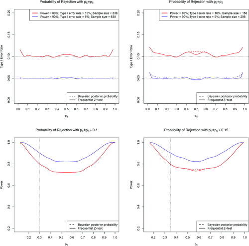
As a numerical illustration, we set Type I error rates at 10% and 5% and target power at 80% and 90% when $(p_S,p_E)=(0.2,0.3)$ and $(p_S,p_E)=(0.2,0.35)$, respectively. To achieve the desired power, the required sample size per arm is $$n=\frac{{(z_{\alpha }+z_{\beta })}^2}{{\delta }^2}\{p_E(1-p_E)+p_S(1-p_S)\},$$ where $\delta =p_E-p_S$. Under the Bayesian design, we assume noninformative prior distributions (e.g., Jeffreys’ prior), $p_S\sim \text{Beta}(0.5,0.5)$ and $p_E\sim \text{Beta}(0.5,0.5)$. For comparison, we compute the Type I error rate and power for both the Bayesian test with $\eta =1-\alpha$ and the frequentist Z-test with a critical value $z_{\alpha }$. As shown in Figure 1, both designs can maintain the Type I error rates at the nominal level and the power at the target level. It is worth noting that because the endpoints are binary and the trial outcomes are discrete, exact calibration of the empirical Type I error rate to the nominal level is not possible, particularly when the sample size is small. When we adopt a larger sample size by setting the Type I error rate to be 5% and the target power to be 90%, the empirical Type I error rate is closer to the nominal level. Due to the discreteness of the Type I error rate formulation, near the boundary points, for example, where p_E = p_S is close to 0 or 1, the Type I error rate might be subject to inflation.

Fig. 1 Comparison of the Type I error rate and power under the frequentist Z-test and Bayesian test based on the posterior probability for detecting treatment difference $\delta =0.1$ (left) and $\delta =0.15$ (right).

3 Hypothesis Test for Binary Data

Following the motivating example in the previous section, the frequentist Z-test for two proportions in (2) leads to the (one-sided test) p-value, $$p{-\text{value}}_1=1-\Phi (Z),$$ where $\Phi (·)$ denotes the cumulative distribution function (CDF) of the standard normal distribution. At the significance level of α, we reject the null hypothesis if p-value is smaller than or equal to α. In the Bayesian paradigm, as given in (3), we reject the null hypothesis if the posterior probability of $H_0:p_E\le p_S$ is smaller than or equal to α; that is, $${\text{PoP}}_1=\mathrm{Pr}(p_E\le p_S|y_E,y_S)\le \alpha .$$

In a numerical study, we set n = 20, 50, 100, and 500, and enumerate all possible integers between 2 and n – 2 to be the values for y_E and y_S (the extreme cases with 0, 1, n – 1, and n are excluded as the p-values cannot be estimated well using normal approximation). We take Jeffreys’ prior for p_E and p_S, that is, $p_E,p_S\sim \text{Beta}(0.5,0.5)$, which is a well-known noninformative prior distribution. 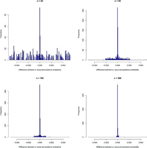For each configuration, we compute the posterior probability of the null hypothesis $\mathrm{Pr}(H_0|y_E,y_S)$ and the p-value. As shown in Figure 2, all the paired values lie very close to the straight line of y = x, indicating the equivalence between the p-value and posterior probability of the null. Figure 3 shows the histograms of differences between p-values and posterior probabilities $\mathrm{Pr}(H_0|y_E,y_S)$ under sample sizes of 20, 50, 100, and 500, respectively. As sample size increases, the distribution of the differences becomes more centered toward 0, further corroborating the asymptotic equivalence relationship.

Fig. 2 The relationship between p-value and the posterior probability of the null in one-sided hypothesis tests with binary outcomes under sample sizes of 20, 50, 100, and 500 per arm, respectively.

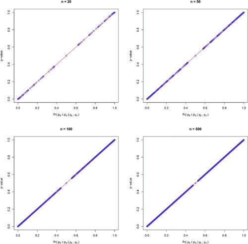
Fig. 3 Histograms of the differences between p-values and posterior probabilities of the null over 1000 replications in one-sided hypothesis tests with binary outcomes under sample sizes of 20, 50, 100, and 500, respectively.

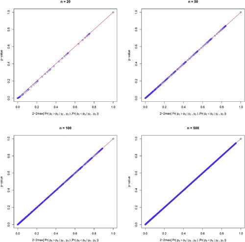
For two-sided hypothesis tests, we are interested in examining whether there is any difference in the treatment effect between the experimental drug and the standard drug, $$H_0:p_E=p_S\hspace{1em}\text{versus}\hspace{1em}{H}_1\text{:}{p}_E\ne p_S,$$ for which the (two-sided test) p-value is given by $$p{-\text{value}}_2=2\{1-\Phi (\left|Z\right|)\}=2[1-\text{max}\{\Phi (Z),\Phi (-Z)\left\}\right].$$

It is worth emphasizing that under the frequentist paradigm, the two-sided test can be viewed as a combination of two one-sided tests along the opposite directions. Therefore, to construct an equivalent counterpart under the Bayesian paradigm, we may regard the problem as two opposite one-sided Bayesian tests and compute the posterior probabilities of the two opposite hypotheses. This approach to Bayesian hypothesis testing is different from those commonly adopted in the literature, where a prior probability mass is imposed on the point null (see, e.g., Berger and Delampady 1987; Berger and Sellke 1987; Berger 2003). If we define the two-sided posterior probability (${\text{PoP}}_2$) as (4) $${\text{PoP}}_2=2[1-\text{max}\{\mathrm{Pr}(p_E>p_S|y_E,y_S),\mathrm{Pr}(p_E<p_S|y_E,y_S)\left\}\right],$$(4) then its equivalence relationship with p-value is similar to that under one-sided hypothesis testing as shown in Figure 4.

Fig. 4 The relationship between p-value and the transformation of the posterior probabilities of the hypotheses in two-sided tests with binary outcomes under sample sizes of 20, 50, 100, and 500, respectively.

The ${\text{PoP}}_2$ in (4) is a transformation of two posterior probabilities of opposite events, and it does not correspond to a single event of interest. However, there exists a sensible interpretation of ${\text{PoP}}_2$ under the Bayesian framework by a simple twist of the definition. Consider a Bayesian test with a point null hypothesis, $H_0:p_E=p_S$ versus $H_1:p_E\cancel{=}{p}_S$. If the null $H_0:p_E=p_S$ is not true, then either p_E > p_S or p_E < p_S is true. In the Bayesian framework, it is natural to compute $\mathrm{Pr}(p_E>p_S|y_E,y_S)$ and $\mathrm{Pr}(p_E<p_S|y_E,y_S)$, and define $${\text{PoP}}_2^{*}=\text{max}\{\mathrm{Pr}(p_E>p_S|y_E,y_S),\mathrm{Pr}(p_E<p_S|y_E,y_S)\},$$ which would be compared to a certain threshold c_T for decision making. If ${\text{PoP}}_2^{*}$ is large enough, then we reject the null hypothesis. Compared with (4), it is easy to show that the decision rule of $${\text{PoP}}_2^{*}\ge c_T=1-\alpha /2,$$ is equivalent to $${\text{PoP}}_2\le \alpha ,$$ which would lead to rejection of the null hypothesis. In this case, ${\text{PoP}}_2$ behaves exactly like p-value in hypothesis testing. That is, by taking $c_T=1-\alpha /2$ and comparing the larger value between $\mathrm{Pr}(p_E>p_S|y_E,y_S)$ and $\mathrm{Pr}(p_E<p_S|y_E,y_S)$ with c_T, we are able to construct a Bayesian test that has an equivalence connection to the frequentist test.

More importantly, the definition of ${\text{PoP}}_2$ is uniquely distinct from the traditional Bayesian hypothesis testing of the two-sided test where H₀ is a point null. Under the traditional Bayesian method, a point mass is typically assigned on the prior distribution of H₀, while various approaches to defining the prior density under H₁ have been discussed (Casella and Berger 1987; Berger and Delampady 1987; Berger and Sellke 1987). Using such an approach, it is difficult to reconcile the classic p-value and the posterior probability. In contrast, instead of assigning a prior probability mass on the point null H₀, our approach to a two-sided hypothesis test takes the maximum of posterior probabilities of two opposite events, under a continuous prior distribution with no probability mass assigned on the point null.

The equivalence of the p-value and the posterior probability in the case of binary outcomes can be established by applying the Bayesian central limit theorem. Under large sample size, the posterior distributions of p_E and p_S can be approximated as $$p_g|y_g\sim \mathrm{N}({\widehat{p}}_g,{\widehat{p}}_g(1-{\widehat{p}}_g)/n),\hspace{1em}g=E,S.$$

As y_E and y_S are independent, the posterior distribution of $p_E-p_S$ can be derived as $$p_E-p_S|y_E,y_S\sim \mathrm{N}({\widehat{p}}_E-{\widehat{p}}_S,\{{\widehat{p}}_E(1-{\widehat{p}}_E)+{\widehat{p}}_S(1-{\widehat{p}}_S)\}/n).$$

Therefore, the posterior probability of $H_0:p_E\le p_S$ is $$\begin{array}{c}{\text{PoP}}_1=\mathrm{Pr}(p_E\le p_S|y_E,y_S)\approx \Phi (-\frac{{\widehat{p}}_E-{\widehat{p}}_S}{{\left[\right\{{\widehat{p}}_E(1-{\widehat{p}}_E)+{\widehat{p}}_S(1-{\widehat{p}}_S)\}/n]}^{1/2}})\\ =\Phi (-Z),\end{array}$$ which is equivalent to $p{-\text{value}}_1=1-\Phi (Z)=\Phi (-Z)$. The equivalence relationship for a two-sided test can be derived along similar lines.

More generally, the equivalence relationship between the posterior probability and $p-\text{value}$ can be derived from the theoretical results in Dudley and Haughton (2002), where the asymptotic normality of the posterior probability of half-spaces is studied. More specifically, a half-space $\mathcal{H}$ is a set satisfying a linear inequality, $$\mathcal{H}=\{\mathrm{\theta }:{\mathbf{a}}^T\mathrm{\theta }\ge b\},$$ where $\mathrm{\theta }\in {\mathbf{R}}^d$ is a vector of interest, $\mathbf{a}\in {\mathbf{R}}^d$, and b is a scalar. Let Δ denote the log likelihood ratio statistic between the unrestricted maximum likelihood estimator (MLE) in the entire support of the parameter and the MLE restricted on the boundary hyperplane of $\mathcal{H}$, $\partial \mathcal{H}=\{\mathrm{\theta }:{\mathbf{a}}^T\mathrm{\theta }=b\}$. Dudley and Haughton (2002) proved that under certain regularity conditions, the posterior probability of a half space converges to the standard normal CDF transformation of the likelihood ratio test statistic, $\Phi (-\sqrt{2\Delta })$. In our case, the half-space under the context of hypothesis testing is $\{(p_E,p_S):p_S-p_E\ge 0\}$ for a two-arm trial with binary endpoints. Based on the arguments in Dudley and Haughton (2002), it can be easily shown that the posterior probability of the null is asymptotically equivalent to the $p-\text{value}$ from the likelihood ratio test.

4 Hypothesis Test for Normal Data

4.1 Hypothesis Test With Known Variance

In a two-arm randomized clinical trial with normal endpoints, we are interested in comparing the means of the outcomes between the experimental and standard arms. Let n denote the sample size for each arm, and let y_Ei and y_Si, $i=1,\dots ,n$, denote the observations in the experimental and standard arms, respectively. We assume that y_Ei and y_Si are independent, and $y_{Ei}\sim \mathrm{N}({\mu }_E,{\sigma }^2)$, $y_{Si}\sim \mathrm{N}({\mu }_S,{\sigma }^2)$, with unknown means μ_E and μ_S but a known variance ${\sigma }^2=1$ for simplicity. Let ${\overline{y}}_E={\sum }_{i=1}^n{y}_{Ei}/n$ and ${\overline{y}}_S={\sum }_{i=1}^n{y}_{Si}/n$ denote the sample means, and let $\theta ={\mu }_E-{\mu }_S$ and $\widehat{\theta }={\overline{y}}_E-{\overline{y}}_S$ denote the true and the observed treatment difference, respectively.

4.1.1 Exact Equivalence

Considering a one-sided hypothesis test, (5) $$H_0\text{:}\theta \le 0\hspace{1em}\text{versus}\hspace{1em}{H}_1\text{:}\theta >0,$$(5) the frequentist test statistic is formulated as $\widehat{\theta }\sqrt{n/2}$, which follows the standard normal distribution under the null hypothesis. Therefore, the p-value under the one-sided hypothesis test is given by (6) $$p{-\text{value}}_1=\mathrm{Pr}(U\ge \widehat{\theta }\sqrt{n/2}|H_0)=1-\Phi (\widehat{\theta }\sqrt{n/2}),$$(6) where U denotes the standard normal random variable.

Let D denote the observed values of y_Ei and y_Si, $i=1,\dots ,n$. In the Bayesian paradigm, if we assume an improper flat prior distribution, $p(\theta )\propto 1$, then the posterior distribution of θ is $$\theta |D\sim \mathrm{N}(\widehat{\theta },2/n).$$

Therefore, the posterior probability of the null is $${\text{PoP}}_1=\mathrm{Pr}(\theta \le 0|D)=1-\Phi (\widehat{\theta }\sqrt{n/2}),$$ which is exactly the same as (6). Under such an improper prior distribution of θ, we can establish an exact equivalence relationship between p-value and $\mathrm{Pr}(H_0|D)$.

Under a two-sided hypothesis test, $$H_0:\theta =0\hspace{1em}\text{versus}\hspace{1em}{H}_1:\theta \ne 0,$$ the p-value is given by (7) $$\begin{array}{c}p{-\text{value}}_2=2[1-\text{max}\{\mathrm{Pr}(U>\widehat{\theta }\sqrt{n/2}|H_0),\\ \mathrm{Pr}(U<\widehat{\theta }\sqrt{n/2}|H_0\left)\right\}]\\ =2-2\text{max}\left\{\Phi \right(-\widehat{\theta }\sqrt{n/2}),\Phi (\widehat{\theta }\sqrt{n/2}\left)\right\}.\end{array}$$(7)

Correspondingly, the two-sided posterior probability is defined as $$\begin{array}{c}{\text{PoP}}_2=2[1-\text{max}\{\mathrm{Pr}(\theta <0|D),\mathrm{Pr}(\theta >0|D)\left\}\right]\\ =2-2\text{max}\left\{\Phi \right(-\widehat{\theta }\sqrt{n/2}),\Phi (\widehat{\theta }\sqrt{n/2}\left)\right\},\end{array}$$ which is exactly the same as the p-value₂ in (7).

4.1.2 Asymptotic Equivalence

If we assume a normal prior distribution, $\theta \sim \mathrm{N}(0,{\sigma }_0^2)$, then the posterior distribution of θ is $\theta |D\sim \mathrm{N}(\tilde{\mu },{\tilde{\sigma }}^2)$, where $$\begin{array}{c}\tilde{\mu }=\frac{n\widehat{\theta }{\sigma }_0^2}{n{\sigma }_0^2+2},\\ {\tilde{\sigma }}^2=\frac{2{\sigma }_0^2}{n{\sigma }_0^2+2}.\end{array}$$

The posterior probability of the null under the one-sided hypothesis test in (5) is $$\begin{array}{c}{\text{PoP}}_1=\mathrm{Pr}(\theta \le 0|D)\\ =1-\Phi (\tilde{\mu }/\tilde{\sigma })\\ =1-\Phi (\widehat{\theta }(n/2)\sqrt{\frac{1}{n/2+1/{\sigma }_0^2}}).\end{array}$$

Therefore, it is evident that as ${\sigma }_0\to \infty$ (i.e., under noninformative priors), the posterior probability of the null converges to the p-value, that is, $p{-\text{value}}_1=\underset{{\sigma }_0^2\to \infty }{\lim }\mathrm{Pr}(\theta \le 0|D).$ For two-sided hypothesis tests, asymptotic equivalence can be derived along similar lines. Moreover, it is worth noting that the same asymptotical equivalence holds when the sample size n goes to infinity, in which case the prior has a negligible effect on the posterior and both the p-value₁ and ${\text{PoP}}_1$ would converge to 0. For one-sided hypothesis testing problems, Casella and Berger (1987) provided theoretical results reconciling the p-value and Bayesian posterior probability for symmetric distributions that enjoy the properties of a monotone likelihood ratio. The results under normal endpoints can be regarded as corroboration of the theoretical findings in Casella and Berger (1987).

4.2 Hypothesis Test With Unknown Variance

In a more general setting, we consider the case where μ_E, μ_S, and σ are all unknown parameters. For simplicity, we define $x_i=y_{Ei}-y_{Si}$, which follows the normal distribution $\mathrm{N}(\theta ,2{\sigma }^2)$ under the independence assumption of y_Ei and y_Si. Similar to a matched-pair study, the problem is reduced to a one-sample test for ease of exposition. In the frequentist paradigm, Student’s t-test statistic is $$T=\frac{\widehat{\theta }}{\sqrt{\sum _{i=1}^n{(x_i-\widehat{\theta })}^2/\{(n-1)n\}}},$$ where $\widehat{\theta }=\overline{x}={\overline{y}}_E-{\overline{y}}_S$. The p-value under the one-sided hypothesis test (5) is $$p{-\text{value}}_1=1-F_{t_{n-1}}(T),$$ where $F_{t_{n-1}}(·)$ denotes the CDF of Student’s t distribution with n – 1 degrees of freedom.

In the Bayesian paradigm, for notational simplicity, we let $\nu =2{\sigma }^2$ and model the joint posterior distribution of θ and ν. Under Jeffreys’ prior for θ and ν, $f(\theta ,\nu )\propto {\nu }^{-3/2}$, the corresponding posterior distribution is $$f(\theta ,\nu |D)\propto {\nu }^{-(n+3)/2}\hspace{0.17em}\text{exp}\hspace{0.17em}\{-\frac{\sum _{i=1}^n{(x_i-\widehat{\theta })}^2+n{(\widehat{\theta }-\theta )}^2}{2\nu }\},$$ which matches the normal-inverse-chi-square distribution, $$(\theta ,\nu )|D\sim \mathrm{N}--\text{Inv}{\chi }^2(\widehat{\theta },n,n,\sum _{i=1}^n{(x_i-\widehat{\theta })}^2/n).$$

As a result, the one-sided posterior probability of the null hypothesis is ${\text{PoP}}_1=\mathrm{Pr}(\theta \le 0|D)$.

To study the influence of prior distributions, we also consider a normal-inverse-gamma prior distribution for θ and ν, $$(\theta ,\nu )\sim \mathrm{N}-\text{IG}({\theta }_0,{\nu }_0,\alpha ,\beta ).$$

The corresponding probability density function (PDF) can be written as the product of a normal density function and an inverse gamma density function, $$\begin{array}{c}f(\theta ,\nu )=f_{\mathrm{N}}(\theta |{\theta }_0,\nu /{\nu }_0)f_{\text{IG}}(\nu |\alpha ,\beta )\\ =\frac{\sqrt{{\nu }_0}}{\sqrt{2\pi \nu }}\frac{{\beta }^{\alpha }}{\Gamma (\alpha )}{(\frac{1}{\nu })}^{\alpha +1}\hspace{0.17em}\text{exp}\hspace{0.17em}(-\frac{2\beta +{\nu }_0{(\theta -{\theta }_0)}^2}{2\nu }),\end{array}$$ where $f_{\mathrm{N}}(·|{\theta }_0,\nu /{\nu }_0)$ denotes the PDF of a normal distribution with mean θ₀ and variance $\nu /{\nu }_0$, and $f_{\text{IG}}(·|\alpha ,\beta )$ denotes that of an inverse gamma distribution with parameters α and β. Due to the conjugate prior property, the corresponding posterior distribution is also a normal-inverse-gamma distribution; that is, $$\begin{array}{c}(\theta ,\nu )|D\sim \mathrm{N}--\text{IG}(\frac{{\theta }_0{\nu }_0+n\widehat{\theta }}{{\nu }_0+n},{\nu }_0+n,\alpha +\frac{n}{2},\\ \hspace{1em}\beta +\frac{1}{2}\sum _{i=1}^n{(x_i-\widehat{\theta })}^2+\frac{n{\nu }_0}{{\nu }_0+n}\frac{{(\widehat{\theta }-{\theta }_0)}^2}{2}).\end{array}$$

For a two-sided hypothesis test, the p-value is $$\begin{array}{c}p{-\text{value}}_2=2-2F_{t_{n-1}}(|T|)\\ =2[1-\text{max}\{F_{t_{n-1}}(T),F_{t_{n-1}}(-T)\left\}\right].\end{array}$$

Similarly, we can define the two-sided posterior probability as $${\text{PoP}}_2=2[1-\text{max}\{\mathrm{Pr}(\theta >0|D),\mathrm{Pr}(\theta <0|D)\left\}\right].$$

4.3 Numerical Studies

As a numerical illustration, we simulate 1000 data replications, and for each replication we compute the p-value and the posterior probability of the null. We consider both Jeffreys’ prior and the normal-inverse-gamma prior. The data are generated from normal distributions, that is, $x_i\sim \mathrm{N}(\theta ,\nu )$. To ensure the p-values from simulations to cover the entire range of (0, 1), we generate values of θ from $\mathrm{N}(0,0.05)$ and ν from truncated $\mathrm{N}(1,0.05)$ above zero. To construct a noninformative normal-inverse-gamma prior distribution, we take ${\theta }_0=0,{\nu }_0=100$, and $\alpha =\beta =0.01$. 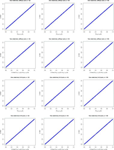Under Jeffreys’ prior and the noninformative normal-inverse-gamma prior distributions, Figure 5 shows the equivalence relationship between p-values and the posterior probabilities of the null under both one- and two-sided tests with sample sizes of 20, 50, and 100, respectively.

Fig. 5 The relationship between p-value and the posterior probability over 1000 replications under one-sided and two-sided hypothesis tests with normal outcomes assuming Jeffreys’ prior and the non-informative normal-inverse-gamma prior under sample sizes of 20, 50, and 100, respectively.

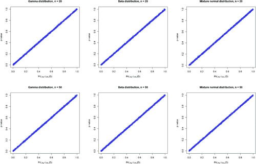
In addition, we conduct sensitivity analysis to explore different data generation distributions and informative priors. In particular, we generate x_i from Gamma$(2,0.5)$, Beta$(0.5,0.5)$, as well as a mixture of normal distributions of N$(-1,1)$ and N(1, 1) with equal weights. To allow the p-values to cover the entire range of (0, 1), the simulated values of x_i are further deducted by the mean of the corresponding distribution. Under Jeffreys’ prior, Figure 6 again exhibits the equivalence relationship between p-values and the posterior probabilities of the null under one-sided tests with sample sizes of 20 and 50, respectively.

Fig. 6 The relationship between p-value and the posterior probability of the null over 1000 replications under one-sided hypothesis tests with outcomes generated from Gamma, Beta, and mixture normal distributions, assuming Jeffreys’ prior for the mean and variance parameters of normal distributions under sample sizes of 20 and 50, respectively.

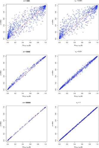
To study the effect of informative prior and sample size on the relationship between p-value and the posterior probability, we assign an informative prior distribution on θ by setting ${\theta }_0=\theta +0.01,{\nu }_0=0.01$ (a small prior variance), and $\alpha =\beta =0.01$. The left panel of Figure 7 shows that under such an informative prior distribution the equivalence relationship between p-values and the posterior probabilities of the null is lost, while it can be gradually gained back with increasing sample sizes. Moreover, we consider the case where the sample size is fixed at 1000 but the prior variance is increased by setting ν₀ from 0.001 to 1, and we still keep ${\theta }_0=\theta +0.01$. The right panel of Figure 7 exhibits that as the prior distribution becomes less informative, the equivalence relationship turns out to be more evident. This is as expected, because the p-value is obtained using the observed data alone without borrowing any prior information, and thus noninformative priors should be used to compute the posterior probability for fair comparisons.

Fig. 7 The relationship between p-value and the posterior probability of the null over 1000 replications under one-sided hypothesis tests with normal outcomes; left panel: assuming a fixed informative normal-inverse-gamma prior under increasing sample sizes of 1000, 10,000, and 100,000 (from top to bottom), right panel: assuming a fixed sample size of 1000 with an increasing prior variance of 0.001, 0.01, and 1 (from top to bottom).

5 Discussion

Berger and Sellke (1987) studied the point null for two-sided hypothesis tests, and noted discrepancies between the frequentist test and the Bayesian test based on the posterior probability. The major difference between their work and ours lies in the specification of the prior distribution. Berger and Sellke (1987) assumed a point mass prior distribution at the point null hypothesis, which violates the regularity condition of continuity in Dudley and Haughton (2002), and thus leads to the discrepancy between the posterior probability and p-value. An underlying condition for our established equivalence is that the union of the support of the parameter under the null and the alternative is the natural whole space of the parameter support, for example, the natural whole space for a normal mean parameter is the real line, that for a probability parameter is (0, 1), and that for a variance parameter is the positive-half real line $(0,\infty )$.

Casella and Berger (1987) provided theoretical results attempting to reconcile the p-value and Bayesian posterior probability in one-sided hypothesis testing problems. Especially, they showed that for certain distributional families the infimum of the Bayesian posterior probability can be reconciled with p-value. Our established equivalence between the p-value and Bayesian posterior probability for normal endpoints can be regarded as more in-depth corroboration of their theoretical results. Furthermore, we demonstrate a similar equivalence relationship for binary endpoints, which was not discussed in Casella and Berger (1987). More importantly, for two-sided hypothesis tests, we establish the notion of the “two-sided posterior probability” by recasting the problem as a combination of two one-sided hypotheses along the opposite directions, which reconnects with the two-sided p-value.

Acknowledgments

We thank the editor Professor Daniel R. Jeske, associate editor, and three referees, for their many constructive and insightful comments that have led to significant improvements in the article. We also thank Chenyang Zhang and Jiaqi Gu for helpful discussions.

Additional information

Funding

The research was supported by a grant (grant number 17307318) for Yin from the Research Grants Council of Hong Kong.

References

- Bayarri, M. J., and Berger, J. O. (2004), “The Interplay of Bayesian and Frequentist Analysis,” Statistical Science, 19, 58–80. DOI: https://doi.org/10.1214/088342304000000116.
- Benjamin, D. J., and Berger, J. O. (2019), “Three Recommendations for Improving the Use of p-Values,” The American Statistician, 73, 186–191. DOI: https://doi.org/10.1080/00031305.2018.1543135.
- Berger, J. O. (2003), “Could Fisher, Jeffreys and Neyman Have Agreed on Testing?” (with discussion), Statistical Science, 18, 1–32. DOI: https://doi.org/10.1214/ss/1056397485.
- Berger, J. O., and Delampady, M. (1987), “Testing Precise Hypotheses,” Statistical Science, 2, 317–335. DOI: https://doi.org/10.1214/ss/1177013238.
- Berger, J. O., and Sellke, T. (1987), “Testing a Point Null Hypothesis: The Irreconcilability of p Values and Evidence,” Journal of the American Statistical Association, 82, 112–122. DOI: https://doi.org/10.2307/2289131.
- Betensky, R. A. (2019), “The p-Value Requires Context, Not a Threshold,” The American Statistician, 73, 115–117. DOI: https://doi.org/10.1080/00031305.2018.1529624.
- Briggs, W. M. (2017), “The Substitute for p-Values,” Journal of the American Statistical Association, 112, 897–898. DOI: https://doi.org/10.1080/01621459.2017.1311264.
- Billheimer, D. (2019), “Predictive Inference and Scientific Reproducibility,” The American Statistician, 73, 291–295. DOI: https://doi.org/10.1080/00031305.2018.1518270.
- Casella, G., and Berger, R. L. (1987), “Reconciling Bayesian and Frequentist Evidence in the One-Sided Testing Problem” (with discussion), Journal of the American Statistical Association, 82, 106–111. DOI: https://doi.org/10.1080/01621459.1987.10478396.
- Colquhoun, D. (2014), “An Investigation of the False Discovery Rate and the Misinterpretation of p-Values,” Royal Society of Open Science, 1, 140–216.
- Concato, J., and Hartigan, J. A. (2016), “P Values: From Suggestion to Superstition,” Journal of Investigative Medicine, 64, 1166–1171. DOI: https://doi.org/10.1136/jim-2016-000206.
- Cumming, G. (2014), “The New Statistics: Why and How,” Psychological Science, 25, 7–29. DOI: https://doi.org/10.1177/0956797613504966.
- Donahue, R. M. J. (1999), “A Note on Information Seldom Reported via the P Value,” The American Statistician, 53, 303–306. DOI: https://doi.org/10.2307/2686048.
- Dudley, R. M., and Haughton, D. (2002), “Asymptotic Normality With Small Relative Errors of Posterior Probabilities of Half-Spaces,” The Annals of Statistics, 30, 1311–1344. DOI: https://doi.org/10.1214/aos/1035844978.
- Fidler, F., Thomason, N., Cumming, G., Finch, S., Leeman, J. (2004), “Editors Can Lead Researchers to Confidence Intervals, But Can’t Make Them Think: Statistical Reform Lessons From Medicine,” Psychological Science, 15, 119–126. DOI: https://doi.org/10.1111/j.0963-7214.2004.01502008.x.
- Gill, J. (2018), “Comments From the New Editor,” Political Analysis, 26, 1–2. DOI: https://doi.org/10.1017/pan.2017.41.
- Goodman, S. N. (1999), “Toward Evidence-Based Medical Statistics. 1: The p Value Fallacy,” Annals of Internal Medicine, 130, 995–1004. DOI: https://doi.org/10.7326/0003-4819-130-12-199906150-00008.
- Hubbard, R., and Lindsay, R. M. (2008), “Why P Values Are Not a Useful Measure of Evidence in Statistical Significance Testing,” Theory & Psychology, 18, 69–88. DOI: https://doi.org/10.1177/0959354307086923.
- Hung, H. J., O’Neill, R. T., Bauer, P., and Kohne, K. (1997), “The Behavior of the p-Value When the Alternative Hypothesis Is True,” Biometrics, 53, 11–22. DOI: https://doi.org/10.2307/2533093.
- Ioannidis, J. P. (2005), “Why Most Published Research Findings Are False,” PLoS Medicine, 2, 124. DOI: https://doi.org/10.1371/journal.pmed.0020124.
- Jager, L. R., and Leek, J. T. (2014), “An Estimate of the Science-Wise False Discovery Rate and Application to the Top Medical Literature,” Biostatistics, 15, 1–12. DOI: https://doi.org/10.1093/biostatistics/kxt007.
- Johnson, V. E. (2013), “Revised Standards for Statistical Evidence,” Proceedings of the National Academy of Sciences of the United States of America, 110, 19313–19317. DOI: https://doi.org/10.1073/pnas.1313476110.
- Leek, J., McShane, B. B., Gelman, A., Colquhoun, D., Nuijten, M. B., and Goodman, S. N. (2017), “Five Ways to Fix Statistics,” Nature, 551, 557–559. DOI: https://doi.org/10.1038/d41586-017-07522-z.
- Lehmann, E. L., and Romano, J. P. (2005), Testing Statistical Hypotheses, New York: Springer.
- Lindley, D. V. (1957), “A Statistical Paradox,” Biometrika, 44, 187–192. DOI: https://doi.org/10.1093/biomet/44.1-2.187.
- Manski, C. F. (2019), “Treatment Choice With Trial Data: Statistical Decision Theory Should Supplant Hypothesis Testing,” The American Statistician, 73, 296–304. DOI: https://doi.org/10.1080/00031305.2018.1513377.
- Matthews, R. A. J. (2019), “Moving Towards the Post p < 0.05 Era via the Analysis of Credibility,” The American Statistician, 73, 202–212.
- McShane, B. B., Gal, D., Gelman, A., Robert, C., and Tackett, J. L. (2019), “Abandon Statistical Significance,” The American Statistician, 73, 235–245. DOI: https://doi.org/10.1080/00031305.2018.1527253.
- Murtaugh, P. A. (2014), “In Defense of P Values,” Ecology, 95, 611–617. DOI: https://doi.org/10.1890/13-0590.1.
- Nuzzo, R. (2014), “Statistical Errors: P Values, the ‘Gold Standard’ of Statistical Validity, Are Not as Reliable as Many Scientists Assume,” Nature, 506, 150–152.
- Pratt, J. W. (1965), “Bayesian Interpretation of Standard Inference Statements” (with discussion), Journal of the Royal Statistical Society, Series B, 27, 169–203. DOI: https://doi.org/10.1111/j.2517-6161.1965.tb01486.x.
- Ranstam, J. (2012), “Why the p-Value Culture Is Bad and Confidence Intervals a Better Alternative,” Osteoarthritis Cartilage, 20, 805–808. DOI: https://doi.org/10.1016/j.joca.2012.04.001.
- Rosenthal, R., and Rubin, D. B. (1983), “Ensemble-Adjusted p Values,” Psychological Bulletin, 94, 540–541. DOI: https://doi.org/10.1037/0033-2909.94.3.540.
- Royall, R. M. (1986), “The Effect of Sample Size on the Meaning of Significance Tests,” The American Statistician, 40, 313–315. DOI: https://doi.org/10.2307/2684616.
- Rubin, D. B. (1984), “Bayesianly Justifiable and Relevant Frequency Calculations for the Applies Statistician,” The Annals of Statistics, 12, 1151–1172. DOI: https://doi.org/10.1214/aos/1176346785.
- Rubin, D. B. (1998), “More Powerful Randomization-Based p-Values in Double-Blind Trials With Non-Compliance,” Statistics in Medicine, 17, 371–385.
- Sackrowitz, H., and Samuel-Cahn, E. (1999), “P Values as Random Variable-Expected P Values,” The American Statistician, 53, 326–331. DOI: https://doi.org/10.2307/2686051.
- Savalei, V., and Dunn, E. (2015), “Is the Call to Abandon p-Values the Red Herring of the Replicability Crisis?,” Frontiers in Psychology, 6, 245. DOI: https://doi.org/10.3389/fpsyg.2015.00245.
- Schervish, M. J. (1996), “P Values: What They Are and What They Are Not,” The American Statistician, 50, 203–206. DOI: https://doi.org/10.2307/2684655.
- Sellke, T., Bayarri, M. J., and Berger, J. O. (2001), “Calibration of p-Values for Testing Precise Null Hypotheses,” The American Statistician, 55, 62–71. DOI: https://doi.org/10.1198/000313001300339950.
- Simmons, J. P., Nelson, L. D., and Simonsohn, U. (2011), “False-Positive Psychology: Undisclosed Flexibility in Data Collection and Analysis Allows Presenting Anything as Significant,” Psychological Science, 22, 1359–1366. DOI: https://doi.org/10.1177/0956797611417632.
- Trafimow, D., Amrhein, V., Areshenkoff, C. N., Barrera-Causil, C. J., Beh, E. J., Bilgiç, Y. K., Bono, R., Bradley, M. T., Briggs, W. M., Cepeda-Freyre, H. A., and Chaigneau, S. E. (2018), “Manipulating the Alpha Level Cannot Cure Significance Testing,” Frontiers in Psychology, 9, 699. DOI: https://doi.org/10.3389/fpsyg.2018.00699.
- Trafimow, D., and Marks, M. (2015), “Editorial,” Basic and Applied Social Psychology, 37, 1–2. DOI: https://doi.org/10.1080/01973533.2015.1012991.
- Wagenmakers, E. J. (2007), “A Practical Solution to the Pervasive Problems of p Values,” Psychonomic Bulletin & Review, 14, 779–804. DOI: https://doi.org/10.3758/BF03194105.
- Wasserstein, R. L., and Lazar, N. A. (2016), “The ASA’s Statement on p-Values: Context, Process, and Purpose,” The American Statistician, 70, 129–133. DOI: https://doi.org/10.1080/00031305.2016.1154108.