A Generalization of the Savage–Dickey Density Ratio for Testing Equality and Order Constrained Hypotheses

ABSTRACT

The Savage–Dickey density ratio is a specific expression of the Bayes factor when testing a precise (equality constrained) hypothesis against an unrestricted alternative. The expression greatly simplifies the computation of the Bayes factor at the cost of assuming a specific form of the prior under the precise hypothesis as a function of the unrestricted prior. A generalization was proposed by Verdinelli and Wasserman such that the priors can be freely specified under both hypotheses while keeping the computational advantage. This article presents an extension of this generalization when the hypothesis has equality as well as order constraints on the parameters of interest. The methodology is used for a constrained multivariate t-test using the JZS Bayes factor and a constrained hypothesis test under the multinomial model.

KEYWORDS:

• Bayes factors
• Constrained hypotheses
• Constrained multinomial models
• Constrained multivariate Bayesian t-test

1 Introduction

The Savage–Dickey density ratio (Dickey 1971) is a special expression of the Bayes factor, the Bayesian measure of statistical evidence between two statistical hypotheses in light of the observed data (Jeffreys 1961; Kass and Raftery 1995). The Savage–Dickey density ratio is relatively easy to compute from Markov chain Monte Carlo (MCMC) output without requiring the marginal likelihoods under the hypotheses. Consider a test of a normal mean θ with unknown variance ${\sigma }^2,H_c:\theta =0$ versus $H_u:\theta \in \mathbb{R}$, with independent observations $y_i\sim N(\theta ,{\sigma }^2)$, for $i=1,\dots ,n$. The indices “c” and “u” refer to a constrained hypothesis and an unconstrained hypothesis.¹ Denote the priors for the unknown parameters under H_c and H_u by ${\pi }_c({\sigma }^2)$ and ${\pi }_u(\theta ,{\sigma }^2)$, respectively, which reflect which values for the parameters are likely before observing the data. Under H_u we consider a unit information prior ${\pi }_u(\theta |{\sigma }^2)=N(0,{\sigma }^2)$ and a conjugate inverse gamma prior for the nuisance parameter, say, ${\pi }_u({\sigma }^2)=IG(\frac{1}{2},\frac{1}{2})$ (the exact choice of the hyperparameters does not qualitatively affect the argument; see, e.g., Verdinelli and Wasserman 1995). The marginal prior for θ under H_u then follows a Cauchy distribution (equivalent to a Student’s t-distribution with 1 degree of freedom) centered at θ = 0 with a scale parameter of 1. The marginal posterior for θ under H_u, ${\pi }_u(\theta |\mathbf{y})$, also has a Student’s t-distribution. When the prior for the nuisance parameter ${\sigma }^2$ under H_c equals the conditional prior for ${\sigma }^2$ under H_u given the restriction under H_c, that is, ${\pi }_c({\sigma }^2)={\pi }_u({\sigma }^2|\theta =0)$, the Bayes factor for H_c against H_u can then be written as the Savage–Dickey density ratio: the ratio of the unconstrained posterior and unconstrained prior density evaluated at the constrained null value under H_c (Dickey 1971), that is,$$B_{cu}=\frac{p_c(\mathbf{y})}{p_u(\mathbf{y})}=\frac{\int p(\mathbf{y}|0,{\sigma }^2){\pi }_1({\sigma }^2)d{\sigma }^2}{\iint p(\mathbf{y}|\theta ,{\sigma }^2){\pi }_u(\theta ,{\sigma }^2)d\theta d{\sigma }^2}=\frac{{\pi }_u(\theta =0|\mathbf{y})}{{\pi }_u(\theta =0)},$$where $p(\mathbf{y}|\theta ,{\sigma }^2)$ denotes the likelihood of the data given the normal mean θ and variance ${\sigma }^2$, and $p_c(\mathbf{y})$ and $p_u(\mathbf{y})$ denote the marginal likelihoods under H_c and H_u, respectively. For the current problem, we would thus need to divide the posterior t distribution of θ under H_u evaluated at θ = 0 by the prior Cauchy distribution at θ = 0, which both have analytic expressions. Note, of course, that the same expression would be obtained by deriving the marginal likelihoods which also have analytic expressions in this scenario. For more complex statistical models with more nuisance parameters, for which the marginal likelihoods would not have analytic expressions, the Savage–Dickey density ratio is particularly useful as we only need to compute the ratio of the unconstrained posterior and the unconstrained prior evaluated at the constrained null value, which are generally easy to obtain, for example, using MCMC output.

Despite its computational convenience, a limitation of the Savage–Dickey density ratio is that it only holds for a specific form of the prior for the nuisance parameters under the restricted model which is completely determined by the prior under the unrestricted model. This imposed prior under the restricted model may not always have a desirable interpretation. For example, for the Savage–Dickey ratio to hold in the above example, the prior for the population variance under H_c equals ${\pi }_c({\sigma }^2)={\pi }_u({\sigma }^2|\theta =0)=IG(1,\frac{1}{2})$. This prior under H_c is more concentrated around smaller values for ${\sigma }^2$ than under H_u as can be seen from the prior modes for ${\sigma }^2$ under H_c and H_u which are $\frac{1}{4}$ and $\frac{1}{3}$, respectively. This is contradictory however because the sample estimate for ${\sigma }^2$ will always be smaller under H_u where the mean θ is unrestricted. Therefore, the Savage–Dickey density ratio should be used with care. For discussions on the Savage–Dickey density ratio, see Marin and Robert (2010) and Heck (2019). For discussions on priors for the nuisance parameters, see Consonni and Veronese (2008).

To retain the computational convenience of the Savage–Dickey density ratio, while allowing researchers to freely specify the prior for the nuisance parameters under the restricted model, Verdinelli and Wasserman (1995) proposed a generalization. In a multivariate setting when testing a vector of key parameters $\mathit{\theta }$, that is, $H_c:\mathit{\theta }=\mathbf{r}$, where r is a vector of constants, against an unconstrained alternative, $H_u:\mathit{\theta }$ unconstrained, with nuisance parameters $\mathit{\varphi }$, where the priors under H_c and H_u are denoted by ${\pi }_c(\mathit{\varphi })$ and ${\pi }_u(\mathit{\theta },\mathit{\varphi })$, respectively, the multivariate generalized Savage–Dickey density ratio is given by(1) $$B_{1u}=\frac{{\pi }_u(\mathit{\theta }=\mathbf{r}|\mathbf{y})}{{\pi }_u(\mathit{\theta }=\mathbf{r})}\times \mathbb{E}\left\{\frac{{\pi }_c(\mathit{\varphi })}{{\pi }_u(\mathit{\varphi }|\mathit{\theta }=\mathbf{r})}\right\},$$(1) where the expectation is taken over the conditional posterior under the unconstrained model, ${\pi }_u(\mathit{\varphi }|\mathit{\theta }=\mathbf{r},\mathbf{y})$. As can be seen, the generalization is equal to the original Savage Dickey density ratio (the first factor on the right hand side of (1)) multiplied with a correction factor based on the ratio of the freely chosen prior for the nuisance parameters, ${\pi }_c(\mathit{\varphi })$, and the imposed prior for the nuisance parameters under the Savage–Dickey density ratio, ${\pi }_u(\mathit{\varphi }|\mathit{\theta }=\mathbf{r})$. In the above example, one might want to use the same marginal prior for the nuisance parameter under H_c as under H_u, that is, ${\pi }_c({\sigma }^2)=IG(\frac{1}{2},\frac{1}{2})$.

The generalization in (1) was not derived when the constrained hypothesis contains order (or one-sided) constraints in addition to equality constraints, say, $H_c:{\mathit{\theta }}_e={\mathbf{r}}_e\&{\mathit{\theta }}_o>{\mathbf{r}}_o$. Scientific theories however are very often formulated with combinations of equality and order constraints (Hoijtink 2011). In repeated measures studies, for instance, theory may suggest a specific ordering of the measurement means (de Jong, Rigotti, and Mulder 2017) or measurement variances (Böing-Messing and Mulder 2020), in a regression model theory may suggest that a certain set of predictor variables have zero effects, while other variables are expected to have a positive or a negative effects (Mulder and Olsson-Collentine 2019), or order constraints may be formulated on regression effects (Haaf and Rouder 2017) or intraclass correlations (Mulder and Fox 2013, 2019) in multilevel models. The goal of the current article is therefore to show the generalization of the Savage–Dickey density ratio in (1) for a constrained hypothesis with equality and order constraints on certain key parameters. This is shown in Section 2, where the generalization is related to existing special cases of the Bayes factor. Section 3 presents two applications of Bayesian constrained hypothesis testing under two statistical models: A multivariate Bayesian t-test for standardized effects under the multivariate normal model using a novel extension of the JZS Bayes factor (Rouder et al. 2009), and a constrained hypothesis test on the cell probabilities under a multinomial model. The article ends with some short concluding remarks in Section 4.

2 Extending the Savage–Dickey Density Ratio

Lemma 1

presents our main result.

Lemma 1. Consider a constrained statistical model, H_c, where the parameters ${\mathit{\theta }}_e$ are fixed with equality constraints, that is, ${\mathit{\theta }}_e={\mathbf{r}}_e$, and order (or one-sided) constraints are formulated on the parameters ${\mathit{\theta }}_o$, that is, ${\mathit{\theta }}_o>{\mathbf{r}}_o$, with (unconstrained) nuisance parameters $\mathit{\varphi }$, and an alternative unconstrained model H_u, where $({\mathit{\theta }}_e,{\mathit{\theta }}_o,\mathit{\varphi })$ are unrestricted. If we denote the priors under H_c and H_u according to ${\pi }_c({\mathit{\theta }}_o,\mathit{\varphi })$ and ${\pi }_u({\mathit{\theta }}_e,{\mathit{\theta }}_o,\mathit{\varphi })$, respectively, then the Bayes factor of model H_c against model H_u given a dataset y can be expressed as(2) $$\begin{array}{c}{B}_{cu}=\frac{{\pi }_u({\mathit{\theta }}_e={\mathbf{r}}_e|\mathbf{y})}{{\pi }_u({\mathit{\theta }}_e={\mathbf{r}}_e){\text{Pr}}_{c^{*}}({\mathit{\theta }}_o>{\mathbf{r}}_o)}\\ \hspace{1em}\times \mathbb{E}\left\{\frac{{\pi }_{c^{*}}({\mathit{\theta }}_o,\mathit{\varphi })}{{\pi }_u({\mathit{\theta }}_o,\mathit{\varphi }|{\mathit{\theta }}_e={\mathbf{r}}_e)}{1}_{\{{\mathit{\theta }}_o>{\mathbf{r}}_o\}}({\mathit{\theta }}_o)\right\},\end{array}$$(2) where the expectation is taken over the conditional posterior of $({\mathit{\theta }}_o,\mathit{\varphi })$ given ${\mathit{\theta }}_e={\mathbf{r}}_e$ under H_u, that is, ${\pi }_u({\mathit{\theta }}_o,\mathit{\varphi }|\mathbf{y},{\mathit{\theta }}_e={\mathbf{r}}_e)$, and ${\pi }_{c^{*}}({\mathit{\theta }}_o,\mathit{\varphi })$ denotes the “completed” prior under the completed constrained hypothesis where the one-sided constraints are omitted, that is, $H_{c^{*}}:{\mathit{\theta }}_e={\mathbf{r}}_e$, such that ${\pi }_c({\mathit{\theta }}_o,\mathit{\varphi })={\text{Pr}}_{c^{*}}{({\mathit{\theta }}_o>{\mathbf{r}}_o)}^{-1}{\pi }_{c^{*}}({\mathit{\theta }}_o,\mathit{\varphi })1_{\{{\mathit{\theta }}_o>{\mathbf{r}}_o\}}({\mathit{\theta }}_o)$, where $1_{\{{\mathit{\theta }}_o>{\mathbf{r}}_o\}}({\mathit{\theta }}_o)$ is the indicator function which equals 1 if ${\mathit{\theta }}_o>{\mathbf{r}}_o$ holds, and 0 otherwise, and ${\text{Pr}}_{c^{*}}(·)$ denotes the prior probability of ${\mathit{\theta }}_o>{\mathbf{r}}_o$ under the completed prior under $H_{c^{*}}$.

Proof. A

ppendix A. □

Remark 1. N

ote that in the special case where$${\pi }_c({\mathit{\theta }}_o,\mathit{\varphi })={\pi }_u({\mathit{\theta }}_o,\mathit{\varphi }|{\mathit{\theta }}_e={\mathbf{r}}_e){\text{Pr}}_u{({\mathit{\theta }}_o>{\mathbf{r}}_o|{\mathit{\theta }}_e={\mathbf{r}}_e)}^{-1}{1}_{\{{\mathit{\theta }}_o>{\mathbf{r}}_o\}}({\mathit{\theta }}_o),$$so that the completed prior under $H_{c^{*}}$ is equal to ${\pi }_u({\mathit{\theta }}_o,\mathit{\varphi }|{\mathit{\theta }}_e={\mathbf{r}}_e)$, then (2) results in the known generalization of the Savage–Dickey density ratio of the Bayes factor for an equality and order hypothesis against an unconstrained alternative,(3) $$B_{cu}=\frac{{\pi }_u({\mathit{\theta }}_e={\mathbf{r}}_e|\mathbf{y})}{{\pi }_u({\mathit{\theta }}_e={\mathbf{r}}_e)}\times \frac{{\text{Pr}}_u({\mathit{\theta }}_o>{\mathbf{r}}_o|\mathbf{y},{\mathit{\theta }}_e={\mathbf{r}}_e)}{{\text{Pr}}_u({\mathit{\theta }}_o>{\mathbf{r}}_o|{\mathit{\theta }}_e={\mathbf{r}}_e)}.$$(3)

This expression has been reported in Mulder and Gelissen (2018), for example.

Remark 2.

In the special case with no order constraints, the parameters ${\mathit{\theta }}_o$ would be part of the nuisance parameters $\mathit{\varphi }$, and thus (2) becomes equal to (1).

Remark 3.

The importance of the “completed” prior where the one-sided constraints are omitted was also highlighted by Pericchi, Liu, and Torres (2008) for intrinsic Bayes factors.

Lemma 1

shows which four ingredients need to be computed to obtain the Bayes factor of a constrained hypothesis against an unconstrained alternative. The computation of these four ingredients can be done in different ways across different statistical models. To give readers more insights about the computational aspects, the next section shows the application of the result under two different statistical models: the multivariate normal model for multivariate continuous data and the multinomial model for categorical data.

3 Applications

3.1 A Multivariate t-Test Using the JZS Bayes Factor

The Cauchy prior for standardized effects is becoming increasingly popular for Bayes factor testing in the social and behavioral sciences (Rouder et al. 2009, 2012; Rouder and Morey 2015). This Bayes factor is based on key contributions by Jeffreys (1961), Zellner and Siow (1980), and Liang et al. (2008), and is therefore also referred to as the JZS Bayes factor. Here, we extend this to a Bayesian multivariate t-test under the multivariate normal model, and show how to compute the Bayes factor for testing a hypothesis with equality and order constraints on the standardized effects using Lemma 1. Note that this test differs from multivariate t-tests on multiple coefficients using a multivariate Cauchy prior under univariate linear regression models (Rouder and Morey 2015; Heck 2019) as we consider a model with a multivariate outcome variable.

Let a multivariate dependent variable of p dimensions, ${\mathbf{y}}_i$, follow a multivariate normal distribution, that is, ${\mathbf{y}}_i\sim N(\mathit{\mu },\mathbf{\Sigma })$, for $i=1,\dots ,n$. To explicitly model the standardized effects, we reparameterize the model according to(4) $${\mathbf{y}}_i\sim N({\mathbf{L}}_{\mathbf{\Sigma }}\mathit{\delta },\mathbf{\Sigma }),$$(4) where $\mathit{\delta }$ are the unknown standardized effects, and ${\mathbf{L}}_{\mathbf{\Sigma }}$ is the lower triangular Cholesky factor of the unknown covariance matrix $\mathbf{\Sigma }$, such that ${\mathbf{L}}_{\mathbf{\Sigma }}{\mathbf{L}}_{\mathbf{\Sigma }}^{\prime }=\mathbf{\Sigma }$. The model in (4) is a generalization of the univariate model considered by Rouder et al. (2009), $y_i\sim N(\sigma \delta ,{\sigma }^2)$.

As a motivating example we consider the bivariate dataset (p = 2) presented in Larocque and Labarre (2004), where ${\mathbf{y}}_i=(y_{i1},y_{i2})\prime$ contains the cell count differences of CD45RA T and CD45RO T cells of n = 36 HIV-positive newborn infants (Sleasman et al. 1999). We are interested in testing whether the standardized effects of the cell count differences of the two cell types are equal and positive, that is,$$\begin{array}{c}{H}_c:{\delta }_1={\delta }_2>0\\ H_u:({\delta }_1,{\delta }_2)\in {\mathbb{R}}^2.\end{array}$$

The sample means were $\overline{\mathbf{y}}=(86.94,193.47)\prime$ and the estimated covariance matrix equaled $\widehat{\mathbf{\Sigma }}=[2019723515;23515106350]$.

Extending the prior proposed by Rouder et al. (2009) to the multivariate normal model, we set an unconstrained Cauchy prior on $\mathit{\delta }$ under H_u and the Jeffreys’ prior for the covariance matrix:$$\begin{array}{c}{\pi }_u(\mathit{\delta },\mathbf{\Sigma })={\pi }_u(\mathit{\delta })\times {\pi }_u(\mathbf{\Sigma })\\ =\text{Cauchy}(\mathit{\delta }|{\mathbf{S}}_{u,0})\times |\mathbf{\Sigma }{|}^{-\frac{p+1}{2}}.\end{array}$$

A diagonal prior scale matrix is set for δ given by ${\mathbf{S}}_{u,0}=\text{diag}(s_1^2,s_2^2)$, with $s_1^2=s_2^2=0.25$. This prior implies that standardized effects of about 0.5 are likely under H_u. Under the constrained hypothesis H_c, the free parameters are the common standardized effect, say, $\delta ={\delta }_1={\delta }_2$, and the error covariance matrix, $\mathbf{\Sigma }$. We set a univariate Cauchy prior for δ with scale s₁ truncated in $\delta >0$, and the Jeffreys’ prior for $\mathbf{\Sigma }$, that is,$$\begin{array}{c}{\pi }_c(\delta ,\mathbf{\Sigma })={\pi }_1(\delta )\times {\pi }_1(\mathbf{\Sigma })\\ =2\times \text{Cauchy}(\delta |s_1)\times 1(\delta >0)\times |\mathbf{\Sigma }{|}^{-\frac{p+1}{2}},\end{array}$$where ${\pi }_{c^{*}}(\delta )=\text{Cauchy}(\delta |s_1)$ denotes the completed prior, and 2 serves as a normalizing constant for the completed prior as ${\text{Pr}}_{c^{*}}{(\delta >0)}^{-1}=2$. As δ has a similar interpretation as δ₁ and δ₂ under H_u, the prior scale is also set to $s_1=0.5$.

By applying the following linear transformation on the standardized effects,(5) $$\mathit{\theta }=\left[\begin{array}{c}{\theta }_e\\ {\theta }_o\end{array}\right]=\left[\begin{array}{c}{\delta }_1-{\delta }_2\\ {\delta }_2\end{array}\right]\left[\begin{array}{cc}1& -1\\ 0& 1\end{array}\right]\left[\begin{array}{c}{\delta }_1\\ {\delta }_2\end{array}\right]=\mathbf{T}\mathit{\delta },$$(5) the model can equivalently be written as ${\mathbf{y}}_i\sim N(\mathbf{L}{\mathbf{T}}^{-1}\mathit{\theta },\mathbf{\Sigma })$, and the hypotheses can be written as$$\begin{array}{c}{H}_c:{\theta }_e=0,{\theta }_o>0\\ H_u:({\theta }_e,{\theta }_o)\in {\mathbb{R}}^2.\end{array}$$

Note here that θ_o corresponds to the common standardized effect δ under H_c. The prior for $({\theta }_e,{\theta }_o)$ under H_u follows a bivariate Cauchy distribution with scale matrix $\mathbf{T}{\mathbf{S}}_{u,0}\mathbf{T}\prime =[0.5-0.25;-0.250.25]$.

If one would be testing the hypotheses with the Savage–Dickey density ratio in (3), it is easy to show that the implied prior for δ under H_c (i.e., the conditional unconstrained prior for θ_o given ${\theta }_e=0$ under H_u) follows a Student’s t-distribution with 2 degrees of freedom with a scale parameter of ${0.25}^2=0.125$; thus assuming that standardized effects of 0.25 are likely under H_c. As was discussed earlier, there is no logical reason why the common standardized effect under the restricted hypothesis H_c is expected to be smaller than the standardized effects under H_u a priori.

The JSZ Bayes factor for this constrained testing problem using Lemma 1 based on the actual Cauchy priors for the standardized effects can be computed using MCMC output from a sampler under H_u, which is described in Appendix B. The R code for the computation is given in Appendix C.1. The four key quantifies in (2) are computed as follows:

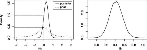
• As the unconstrained marginal prior for θ_e follows a Cauchy distribution with scale $\sqrt{0.5}$ (Figure 1, left panel, dashed line), the prior density equals ${\pi }_u({\theta }_e=0|\mathbf{Y})=\sqrt{2}/\pi$.

• The estimated marginal posterior for θ_e under H_u follows from MCMC output. The estimated posterior for θ_e is plotted in Figure 1 (left panel, solid line). This yields ${\widehat{\pi }}_u({\theta }_e=0|\mathbf{Y})=0.9871618$.

• As the completed prior for δ under $H_{c^{*}}$ follows a $\text{Cauchy}(0.5)$ distribution that is centered at zero, the prior probability equals $P{r}_{c^{*}}(\delta >0)=0.5$.

• As the priors for the covariance matrices cancel out in the fraction, the expected value can be written as $\mathbb{E}\left\{\frac{\text{Cauchy}({\theta }_o|0.5)}{\text{Cauchy}({\theta }_o|0.25)}{1}_{\{{\theta }_o>0\}}({\theta }_o)\right\}$ under the conditional posterior for θ_o given ${\theta }_e=0$ under H_u. Appendix B also shows how to get posterior draws from θ_o under H_u given ${\theta }_e=0$. The estimated posterior is displayed in Figure 1 (right panel). A Monte Carlo estimate can then be used to compute the expectation, which yields 1.098799.

Fig. 1 Estimated probability densities for the multivariate Student’s t-test. Left panel: Marginal posterior (solid line) and prior (dashed line) for ${\theta }_e={\delta }_1-{\delta }_2$. The dotted lines indicate the estimated density values at ${\theta }_e=0$. Right panel: Estimated conditional posterior for θ_o given ${\theta }_e=0$ under H_u.

Application of Lemma 1 then yields a Bayes factor for H_c against H_u of $B_{cu}=\frac{0.9871618}{\sqrt{2}/\pi \times 0.5}\times 1.098799=4.8$. Thus, there is 4.8 times more evidence in the data for equal and positive standardized count differences than for the unconstrained alternative hypothesis. Assuming equal prior probabilities for H_c and H_u this would yield posterior probabilities of $\text{Pr}(H_c|\mathbf{Y})=0.783$ and $\text{Pr}(H_u|\mathbf{Y})=0.217$. Thus, there is mild evidence for H_c relative to H_u. To draw clearer conclusions more data would need to be collected.

3.2 Constrained Hypothesis Testing Under the Multinomial Model

When analyzing categorical data using a multinomial model, researchers are often interested in testing the relationships between the probabilities of the different cells (Robertson 1978; Klugkist, Laudy, and Hoijtink 2010; Heck and Davis-Stober 2019). As an example, we consider an experiment for testing the Mendelian inheritance theory discussed by Robertson (1978). A total of 556 peas coming from crosses of plants from round yellow seeds and plants from wrinkled green seeds were divided in four categories. The cell probabilities for these categories are contained in the vector $\mathit{\gamma }=({\gamma }_1,{\gamma }_2,{\gamma }_3,{\gamma }_4)$, where γ₁ denotes the probability that a pea resulting from such a mating is round and yellow; γ₂ denotes the probability that it is wrinkled and yellow; γ₃ denotes the probability that it is round and green; and γ₄ denotes the probability that it is wrinkled and green. The Mendelian theory states that γ₁ is largest, followed by γ₂ and γ₃ which are assumed to be equal, and γ₄ is expected to be smallest. This can be summarized as $H_c:{\gamma }_1>{\gamma }_2={\gamma }_3>{\gamma }_4$. In particular, the theory dictates that the four probabilities are proportional to 9, 3, 3, and 1, respectively. We translate this to a completed prior under $H_{c^{*}}$ such that its means satisfy $\frac{E({\gamma }_1)}{E({\gamma }_2)}=\frac{E({\gamma }_2)}{E({\gamma }_4)}=3$. This can be achieved via a Dirichlet prior under an alternative parameterization, $({\xi }_1,{\xi }_2,{\xi }_4)\sim \text{Dirichlet}({\alpha }_{c1},{\alpha }_{c2},{\alpha }_{c3})$, with ${\mathit{\alpha }}_c=(9,6,1)\prime$. The cell probabilities under $H_{c^{*}}$ are then defined by $({\gamma }_1,{\gamma }_2,{\gamma }_4)=({\xi }_1,{\xi }_2/2,{\xi }_4)$, which then follow a specific scaled Dirichlet distribution, which we denote by SDirichlet(9, 6, 1).² The prior for the cell probabilities under H_c is then a truncation of this scaled Dirichlet distribution truncated under ${\gamma }_1>{\gamma }_2>{\gamma }_4$. The Mendelian hypothesis can equivalently be formulated on the transformed parameters $({\theta }_e,{\theta }_{o,1},{\theta }_{o,2},\varphi )=({\gamma }_2-{\gamma }_3,{\gamma }_1-{\gamma }_2,{\gamma }_2-{\gamma }_4,{\gamma }_2)$ so that $H_c:{\theta }_e=0,({\theta }_{o,1},{\theta }_{o,2})>0$, as in Lemma 1. It is easier however to compute the four quantities in (2) via the untransformed parameters $\mathit{\gamma }$ as will be shown below.

The Mendelian hypothesis will be tested against an unconstrained alternative which does not make any assumptions about the relationships between the cell probabilities. A uniform prior on the simplex will be used under the alternative, that is, ${\pi }_u({\gamma }_1,{\gamma }_2,{\gamma }_3,{\gamma }_4)=\text{Dirichlet}(1,1,1,1)$. The observed frequencies in the four respective categories were equal to 315, 101, 108, and 32.

The R code for the computation of the Bayes factor of H_c against H_u can be found in Appendix C.2.

• The unconstrained marginal prior density at ${\theta }_e=0$ can be estimated from a sample of ${\theta }_e={\gamma }_2-{\gamma }_3$ where $\mathit{\gamma }$ is sampled from the unconstrained Dirichlet$(1,1,1,1)$ prior, resulting in ${\widehat{\pi }}_u({\theta }_e=0)=1.476556$.

• Similarly, the unconstrained marginal posterior density at ${\theta }_e=0$ can be obtained by sampling $\mathit{\gamma }$ from the unconstrained Dirichlet$(316,102,109,33)$ posterior, resulting in ${\widehat{\pi }}_u({\theta }_e=0|\mathbf{y})=13.71403$.

• The prior probability under H_c can be obtained by first sampling $({\xi }_1,{\xi }_2,{\xi }_4)\sim \text{Dirichlet}(9,6,1)$, then transforming the prior draws according to $({\gamma }_1,{\gamma }_2,{\gamma }_4)=({\xi }_1,{\xi }_2/2,{\xi }_4)$, and taking the proportion of draws satisfying the constraints ${\text{Pr}}_c({\gamma }_1>{\gamma }_2>{\gamma }_3)\approx S^{-1}{\sum }_{s=1}^{S}I({\gamma }_1^{(s)}>{\gamma }_2^{(s)}>{\gamma }_3^{(s)})=0.8949818$, where ${\mathit{\gamma }}^{(s)}$ denotes the sth draw, for $s=1,\dots ,S$.

• To get draws from the conditional distribution $({\gamma }_1,{\gamma }_2,{\gamma }_3,{\gamma }_4)$ given ${\gamma }_2={\gamma }_3$ when $({\gamma }_1,{\gamma }_2,{\gamma }_3,{\gamma }_4)\sim \text{Dirichlet}({\alpha }_1,{\alpha }_2,{\alpha }_3,{\alpha }_4)$ under H_u, we can sample transformed parameters $({\xi }_1,{\xi }_2,{\xi }_4)\sim \text{Dirichlet}({\alpha }_1,{\alpha }_2+{\alpha }_3-1,{\alpha }_4)$, and compute $({\gamma }_1,{\gamma }_2,{\gamma }_3,{\gamma }_4)=({\xi }_1,{\xi }_2/2,{\xi }_2/2,{\xi }_4)$. This can be used to obtain draws from the conditional posterior for $({\gamma }_1,{\gamma }_2,{\gamma }_3,{\gamma }_4)$ given ${\gamma }_2={\gamma }_3$ under H_u by setting $\mathit{\alpha }=(315,101,108,33)$. The expectation in (2) can then be computed as the arithmetic mean of $\frac{\text{SDirichlet}(({\gamma }_1,{\gamma }_2,{\gamma }_4)|\mathit{\alpha }=(9,6,1))}{\text{SDirichlet}(({\gamma }_1,{\gamma }_2,{\gamma }_4)|\mathit{\alpha }=(1,1,1))}I({\gamma }_1>{\gamma }_2>{\gamma }_4)$ based on a sufficiently large sample. This yields an estimate of 10.50881.

In sum the Bayes factor of the Mendelian hypothesis against the noninformative unconstrained alternative is equal to $B_{cu}=\frac{13.71403}{1.476556\times 0.8949818}\times 10.50881=109.0572$. This can be interpreted as relatively strong evidence for the Mendelian hypothesis against an unconstrained alternative based on the observed data.

Finally note that by using probability calculus it can be shown that the first two ingredients have analytic solutions as the marginal probability density at ${\theta }_e={\gamma }_2-{\gamma }_3=0$ under H_u, when $\mathit{\gamma }\sim \text{Dirichlet}(\mathit{\alpha })$, is equal to $\frac{\Gamma ({\alpha }_2+{\alpha }_3)({\alpha }_1+{\alpha }_2+{\alpha }_3+{\alpha }_4-1)}{\Gamma ({\alpha }_2)\Gamma ({\alpha }_3)({\alpha }_2+{\alpha }_3-1)2^{{\alpha }_2+{\alpha }_3-1}}$. In the above calculation, numerical estimates were used to give readers more insights how to obtain these quantities when analytic expressions are unavailable.

4 Concluding Remarks

As Bayes factors are becoming increasingly popular to test hypotheses with equality as well as order constraints on the parameters of interest, more flexible and fast estimation methods to acquire these Bayes factors are needed. The generalization of the Savage–Dickey density ratio that was presented in this article will be a useful contribution for this purpose. The expression allows one to compute Bayes factors in a straightforward manner from MCMC output while being able to freely specify the priors for the free parameters under the competing hypotheses. The applicability of the proposed methodology was illustrated in a constrained multivariate t-test using a novel extension of the JSZ Bayes factor to the multivariate normal model and in a constrained hypothesis test under the multinomial model.

Acknowledgments

The authors would like to thank Florian Böing-Messing for helpful discussions at an early stage of the article, and the editor and three anonymous reviewers for constructive feedback which improved the readability of the article.

Appendix A

Proof of Lemma 1

As the constrained model $H_c:{\mathit{\theta }}_e={\mathbf{r}}_e\&{\mathit{\theta }}_o>{\mathbf{r}}_o$ is nested in the unconstrained model H_u, the likelihood under H_c can be written as the truncation of the unconstrained likelihood, that is, $p_c(\mathbf{y}|{\mathit{\theta }}_o,\mathit{\varphi })=p_u(\mathbf{y}|{\mathit{\theta }}_e={\mathbf{r}}_e,{\mathit{\theta }}_o,\mathit{\varphi })1_{\{{\mathit{\theta }}_o>{\mathbf{r}}_o\}}({\mathit{\theta }}_o)$. The result in Lemma 1 then follows via the following steps,$$\begin{array}{c}{B}_{cu}=\frac{p_c(\mathbf{y})}{p_u(\mathbf{y})}=\frac{{\iint }_{{\mathit{\theta }}_o>{\mathbf{r}}_o}{p}_c(\mathbf{y}|{\mathit{\theta }}_o,\mathit{\varphi }){\pi }_c({\mathit{\theta }}_o,\mathit{\varphi })d{\mathit{\theta }}_{o}d\mathit{\varphi }}{\iiint p_u(\mathbf{y}|{\mathit{\theta }}_e,{\mathit{\theta }}_o,\mathit{\varphi }){\pi }_u({\mathit{\theta }}_e,{\mathit{\theta }}_o,\mathit{\varphi })d{\mathit{\theta }}_{e}d{\mathit{\theta }}_{o}d\mathit{\varphi }}\\ ={\iint }_{{\mathit{\theta }}_o>{\mathbf{r}}_o}\frac{p_u(\mathbf{y}|{\mathit{\theta }}_e={\mathbf{r}}_e,{\mathit{\theta }}_o,\mathit{\varphi })1_{\{{\mathit{\theta }}_o>{\mathbf{r}}_o\}}({\mathit{\theta }}_o){\pi }_c({\mathit{\theta }}_o,\mathit{\varphi })}{p_u(\mathbf{y}){\pi }_u({\mathit{\theta }}_e={\mathbf{r}}_e|\mathbf{y})}d{\mathit{\theta }}_{o}d\mathit{\varphi }\\ \times {\pi }_u({\mathit{\theta }}_e={\mathbf{r}}_e|\mathbf{y})\\ ={\iint }_{{\mathit{\theta }}_o>{\mathbf{r}}_o}\frac{p_u(\mathbf{y}|{\mathit{\theta }}_e={\mathbf{r}}_e,{\mathit{\theta }}_o,\mathit{\varphi }){\pi }_c({\mathit{\theta }}_o,\mathit{\varphi })}{p_u(\mathbf{y}){\pi }_u({\mathit{\theta }}_e={\mathbf{r}}_e,{\mathit{\theta }}_o,\mathit{\varphi }|\mathbf{y})}{\pi }_u({\mathit{\theta }}_o,\mathit{\varphi }|\mathbf{y},{\mathit{\theta }}_e={\mathbf{r}}_e)d{\mathit{\theta }}_{o}d\mathit{\varphi }\\ \times {\pi }_u({\mathit{\theta }}_e={\mathbf{r}}_e|\mathbf{y})\\ ={\iint }_{{\mathit{\theta }}_o>{\mathbf{r}}_o}\frac{{\pi }_c({\mathit{\theta }}_o,\mathit{\varphi })}{{\pi }_u({\mathit{\theta }}_e={\mathbf{r}}_e,{\mathit{\theta }}_o,\mathit{\varphi })}{\pi }_u({\mathit{\theta }}_o,\mathit{\varphi }|\mathbf{y},{\mathit{\theta }}_e={\mathbf{r}}_e)d{\mathit{\theta }}_{o}d\mathit{\varphi }\\ \times {\pi }_u({\mathit{\theta }}_e={\mathbf{r}}_e|\mathbf{y})\\ ={\iint }_{{\mathit{\theta }}_o>{\mathbf{r}}_o}\frac{{\pi }_c({\mathit{\theta }}_o,\mathit{\varphi })}{{\pi }_u({\mathit{\theta }}_o,\mathit{\varphi }|{\mathit{\theta }}_e={\mathbf{r}}_e)}{\pi }_u({\mathit{\theta }}_o,\mathit{\varphi }|\mathbf{y},{\mathit{\theta }}_e={\mathbf{r}}_e)d{\mathit{\theta }}_{o}d\mathit{\varphi }\\ \times \frac{{\pi }_u({\mathit{\theta }}_e={\mathbf{r}}_e|\mathbf{y})}{{\pi }_u({\mathit{\theta }}_e={\mathbf{r}}_e)}\\ =\iint \frac{{\pi }_{c^{*}}({\mathit{\theta }}_o,\mathit{\varphi })1_{\{{\mathit{\theta }}_o>{\mathbf{r}}_o\}}({\mathit{\theta }}_o)}{{\pi }_u({\mathit{\theta }}_o,\mathit{\varphi }|{\mathit{\theta }}_e={\mathbf{r}}_e){\text{Pr}}_{c^{*}}({\mathit{\theta }}_o>{\mathbf{r}}_o)}{\pi }_u({\mathit{\theta }}_o,\mathit{\varphi }|\mathbf{y},{\mathit{\theta }}_e={\mathbf{r}}_e)d{\mathit{\theta }}_{o}d\mathit{\varphi }\\ \times \frac{{\pi }_u({\mathit{\theta }}_e={\mathbf{r}}_e|\mathbf{y})}{{\pi }_u({\mathit{\theta }}_e={\mathbf{r}}_e)}\\ =\iint \frac{{\pi }_{c^{*}}({\mathit{\theta }}_o,\mathit{\varphi })1_{\{{\mathit{\theta }}_o>{\mathbf{r}}_o\}}({\mathit{\theta }}_o)}{{\pi }_u({\mathit{\theta }}_o,\mathit{\varphi }|{\mathit{\theta }}_e={\mathbf{r}}_e)}{\pi }_u({\mathit{\theta }}_o,\mathit{\varphi }|\mathbf{y},{\mathit{\theta }}_e={\mathbf{r}}_e)d{\mathit{\theta }}_{o}d\mathit{\varphi }\\ \times {\text{Pr}}_{c^{*}}{({\mathit{\theta }}_o>{\mathbf{r}}_o)}^{-1}\times \frac{{\pi }_u({\mathit{\theta }}_e={\mathbf{r}}_e|\mathbf{y})}{{\pi }_u({\mathit{\theta }}_e={\mathbf{r}}_e)},\end{array}$$which completes the proof. Note that in the third step the indicator function, $1_{\{{\mathit{\theta }}_o>{\mathbf{r}}_o\}}({\mathit{\theta }}_o)$, was omitted as the integrand is integrated over the subspace where ${\mathit{\theta }}_o>{\mathbf{r}}_o$. In the second last step, the completed version of the constrained hypothesis has the order constraints omitted, that is, $H_{c^{*}}:{\mathit{\theta }}_e={\mathbf{r}}_e$, with completed prior ${\pi }_{c^{*}}({\mathit{\theta }}_o,\mathit{\varphi })$, such that ${\pi }_c({\mathit{\theta }}_o,\mathit{\varphi })={\pi }_{c^{*}}({\mathit{\theta }}_o,\mathit{\varphi }){\text{Pr}}_{c^{*}}{({\mathit{\theta }}_o>{\mathbf{r}}_o)}^{-1}{1}_{\{{\mathit{\theta }}_o>{\mathbf{r}}_o\}}({\mathit{\theta }}_o)$.

Appendix B

MCMC Sampler for the Multivariate Student’s t-test

1. Drawing the standardized effects $\mathit{\delta }$. It is well-known that a multivariate Cauchy prior of p dimensions can be written as a Multivariate normal distribution with an inverse Wishart mixing distribution on the normal covariance matrix with p degrees of freedom, that is,$$\begin{array}{c}{\pi }_u(\mathit{\delta })=\text{Cauchy}(\mathit{\delta }|{\mathbf{S}}_0)\\ =\int N(\mathit{\delta }|0,\mathbf{\Phi })\times \text{IW}(\mathbf{\Phi }|p,{\mathbf{S}}_0)d\mathbf{\Phi }.\end{array}$$

   Thus, the conditional prior for $\mathit{\delta }$ given the auxiliary parameter matrix $\mathbf{\Phi }$ follows a $N(0,\mathbf{\Phi })$ distribution. Consequently, as ${\mathbf{z}}_{\mathbf{\Sigma },i}={\mathbf{L}}_{\mathbf{\Sigma }}^{-1}{\mathbf{y}}_i\sim N(\mathit{\delta },{\mathbf{I}}_p)$, the conditional posterior of $\mathit{\delta }$ follows a multivariate normal posterior,$$\mathit{\delta }|\mathbf{\Phi },\mathbf{\Sigma },\mathbf{y}\sim N(n{({\mathbf{\Phi }}^{-1}+n{\mathbf{I}}_p)}^{-1}{\overline{\mathbf{z}}}_{\mathbf{\Sigma }},{({\mathbf{\Phi }}^{-1}+n{\mathbf{I}}_p)}^{-1}),$$where ${\overline{\mathbf{z}}}_{\mathbf{\Sigma }}$ are the sample means of ${\mathbf{z}}_{\mathbf{\Sigma },i}$, for $i=1,\dots ,n$.

2. Drawing the auxiliary covariance matrix $\mathbf{\Phi }$. The conditional posterior for $\mathbf{\Phi }$ only depends on the standardized effects and it follows an inverse Wishart distribution,$$\mathbf{\Phi }|\mathit{\delta }\sim \text{IW}(p+1,{\mathbf{S}}_0+\mathit{\delta \delta }\prime ).$$

3. Drawing the error covariance matrix $\mathbf{\Sigma }$. The conditional posterior for the covariance matrix does not follow a known distribution. For this reason we use a random walk (e.g., Gelman et al. 2004) for sampling the separate elements of $\mathbf{\Sigma }$.

The sampler under the unconstrained model while restricting ${\delta }_1={\delta }_2$ ($=\delta$) is very similar except that the prior for δ is now univariate Cauchy$(\delta |0.25)$ and $\mathbf{\Phi }=[{\varphi }^2]$ is a scalar, and thus the conditional posterior for δ is univariate normal $N(2n{({\varphi }^{-2}+2n)}^{-1}{\overline{z}}_{\mathbf{\Sigma }},{({\varphi }^{-2}+n)}^{-1})$, where ${\overline{z}}_{\mathbf{\Sigma }}$ is the mean of ${\overline{\mathbf{z}}}_{\mathbf{\Sigma }}$. Also note that the inverse Wishart distribution in Step 2 is now for a 1 × 1 covariance matrix which is equivalent to an inverse gamma distribution.

Appendix C

R Code for Empirical Analyses

C.1 R Code for Multivariate t-Test in Section 3.1

library(mvtnorm) library(Matrix) # computing the unconstrained marginal prior density at\theta_e = 0:priorE <- dcauchy(0, location = 0,scale = sqrt(.5)) # computing the unconstrained marginal posterior density at\theta_e = 0: # read data Y <- t(matrix(c(242,1708,569,569,270,757,-25,499, 309,231,22,338,-42,26,-233,119,206,163,-106, -186,55,54,85,48,30,50,194,525,-87,-110,159, 148,29,102,89,364,-9,36,158,234,76,122,15,24, 3,36,93,71,160,44,66,128,180,155,237,85,105, 76,16,6,167,364,-10,-18,-61,-21,-7,-2,15,32, 160,188), nrow = 2)) set.seed(123) #dimension p <- ncol(Y) nums <- p*(p + 1)/2 n <- nrow(Y) #initial parameter values based on burn-in period delta <- c(.5,.2) Sigma <- matrix(c(2,2,2,11),2,2) * 10**4 L <- t(chol(Sigma)) Phi <- diag(p) #selection of unique elements in\Sigma lowerSigma <- lower.tri(Sigma,diag = TRUE) welklower <- which(lowerSigma) # tranformation matrix Trans <- matrix(c(1,0,-1,1),ncol = 2) #prior hyperparameters S0 <- diag(p) *.5**2 # random walk sd’s for the elements of\Sigma # to have an efficient acceptance probability # based on burn-in period. sdstep <- c(9,13,48) * 10**3 #store draws numdraws <- 1e5 storeDelta <- matrix(0,nrow = numdraws,ncol = p) storeSigma <- storePhi <- array(0,dim = c(numdraws, p,p)) #draws from stationary distribution for(s in 1:numdraws){ #draw delta deltaMean <- c(apply(Y SigmaDelta <- solve(n*diag(p) + solve(Phi)) muDelta <- c(SigmaDelta delta <- c(rmvnorm(1,mean = muDelta,sigma= SigmaDelta)) #draw Phi Phi <- solve(rWishart(1,df = p + 1,Sigma = solve(S0 + delta #draw Sigma using MH for(sig in 1:nums){ welknu <- welklower[sig] step1 <- rnorm(1,sd = sdstep[sig]) Sigma0 <- matrix(0,p,p) Sigma0[lowerSigma] <- Sigma[lowerSigma] Sigma0[welknu] <- Sigma0[welknu] + step1 Sigma_can <- Sigma0 + t(Sigma0) - diag (diag(Sigma0)) if(min(eigen(Sigma_can)$values) >.000001){ #the candidate is positive definite L_can <- t(chol(Sigma_can)) #acceptance probability R_MH <- exp(sum(dmvnorm(Y,mean = c(L_can%* %delta), sigma = Sigma_can, log = TRUE)) - (p + 1)/2*log(det(Sigma_can))- sum(dmvnorm(Y,mean = c(L Sigma,log = TRUE)) + (p + 1)/2*log(det(Sigma))) if(runif(1) < R_MH){ #accept draw Sigma <- Sigma_can L <- t(chol(Sigma))}}} storeDelta[s,] <- delta storeSigma[s,] <- Sigma storePhi[s,] <- Phi} drawsE <- storeDelta[,1] - storeDelta[,2] denspost <- density(drawsE) df <- approxfun(denspost) postE <- df(0) # Figure 1 (left panel) plot(denspost,xlim = c(-3,3),main="",xlab="theta_e") seq1 <- seq(-3,3,length = 1e3) lines(seq1,dcauchy(seq1,scale = sqrt(.5)),lty = 2) # computing the prior probability of\theta_o > 0 under H_c: priorO <- 1 - pcauchy(0, location = 0, scale =.5) # computing the expectation of the ratio of the # priors from a posterior sample under H_c given #\theta_e = 0 initialization set.seed(123) p1 <- 1 p <- ncol(Y) nums <- p*(p + 1)/2 n <- nrow(Y) S0 <- diag(1)*.25**2 # initial parameter values based on burn-in period delta <-.55 Phi <- matrix(1) Sigma <- matrix(c(23,22,22,89),nrow = 2) * 10**3 L <- t(chol(Sigma)) # random walk sd’s for the elements of\Sigma to # have an efficient acceptance probability based # on burn-in period. sdstep1 <- c(10,15,48) * 10**3 lowerSigma <- lower.tri(Sigma,diag = TRUE) welklower <- which(lowerSigma) # store draws numdraws <- 1e5 storeDelta1 <- matrix(0,nrow = numdraws,ncol = 1) storePhi1 <- array(0,dim = c(numdraws,p1,p1)) storeSigma1 <- array(0,dim = c(numdraws,p,p)) for(s in 1:numdraws){ #draw delta deltaMean <- mean(c(apply(Y mean))) SigmaDelta <- solve(2*n*diag(p1) + solve(Phi)) muDelta <- c(SigmaDelta delta <- c(rmvnorm(1,mean = muDelta,sigma= SigmaDelta)) #draw Phi Phi <- solve(rWishart(1,df = p1 + 1,Sigma = solve(S0+ Delta%*% (delta))) [,1]) #draw Sigma using MH deltavec <- rep(delta,2) for(sig in 1:nums){ welknu <- welklower[sig] step1 <- rnorm(1,sd = sdstep1[sig]) Sigma0 <- matrix(0,p,p) Sigma0[lowerSigma] <- Sigma0[lowerSigma] + Sigma[lowerSigma] Sigma0[welknu] <- Sigma0[welknu] + step1 Sigma_can <- Sigma0 + t(Sigma0) - diag(diag(Sigma0)) if(min(eigen(Sigma_can)$values) >.000001){ #the candidate is positive definite L_can <- t(chol(Sigma_can)) #dit zou sneller kunnen via onafhankelijke univariate normals R_MH <- exp(sum(dmvnorm(Y,mean = c(L_can% *%deltavec) sigma = Sigma_can,log = TRUE)) - (p + 1)/2* log(det(Sigma_can)) - sum(dmvnorm(Y,mean = c(L%*%deltavec), sigma = Sigma,log = TRUE)) + (p + 1)/2*log(det(Sigma))) if(runif(1) < R_MH){ #accept draw Sigma <- Sigma_can L <- t(chol(Sigma))}}} storeDelta1[s,] <- delta storePhi1[s,] <- Phi storeSigma1[s,] <- Sigma} expratio <- mean(dcauchy(c(storeDelta1), scale=.5)/dcauchy(c(storeDelta1),scale=.25) * (c(storeDelta1)>0)) # Figure 1, right panel plot(density(c(storeDelta1)),main="", xlab="theta_o") # computation of the Bayes factor Bcu <- postE/(priorE * priorO) * expratio

C.2 R Code for Multinomial Model in Section 3.2

library(MCMCpack) set.seed(123) # computing the unconstrained marginal prior density at\theta_e = 0: uncpriorsample <- rdirichlet(n = 1e7, alpha = c(1,1,1,1)) densprior <- density(uncpriorsample[,2]- uncpriorsample[,3]) df <- approxfun(densprior) priorE <- df(0) remove(uncpriorsample) # computing the unconstrained marginal posterior density at\theta_e = 0:uncpostsample <- rdirichlet(n = 1e7, alpha = c(1 + 315,1 + 101,1 + 108, 1 + 32)) denspost <- density(uncpostsample[,2]- uncpostsample[,3]) df <- approxfun(denspost) postE <- df(0) remove(uncpostsample) # computing the prior probability of\theta_o > 0 under H_c:priorsample1 <- rdirichlet (n = 1e7,alph = c(9,6,1))priorsample1[,2] <- priorsample1[,2]/2 priorO <- mean(priorsample1[,1] > priorsample1[,2] & priorsample1[,2] > priorsample1[,3]) remove(priorsample1) # computing the expectation of the ratio of # priors: first define probability density # for (gamma1,gamma2) SDirichlet <- function(gamma1,gamma2,alpha1, alpha2,alpha3){ alphavec <- c(alpha1,alpha2,alpha3) B1 <- exp(sum(lgamma(alphavec)) - lgamma(sum (alphavec))) return( 2^alpha2/B1 * gamma1^(alpha1-1) * gamma2^(alpha2-1) * (1-gamma1-2*gamma2) ^(alpha3-1) )} condpostsample <- rdirichlet(n = 1e7, alpha = c(316, 210,33)) condpostsample[,2] <- condpostsample[,2]/2 expratio <- mean(SDirichlet(condpostsample[,1], condpostsample[,2],9,6,1)/ SDirichlet(condpostsample[,1],condpostsample [,2],1,1,1) * (condpostsample[,1]>condpostsample[,2] & condpostsample[,2]>condpostsample[,3]) ) remove(condpostsample) # computing the Bayes factor of $H_c$against $H_u$: Bcu <- postE/(priorE*priorO)*expratio

Funding

Mulder is supported by an ERC starting grant (758791).

Notes

¹ The test can equivalently be formulated as a test of $H_c:\theta =0$ versus $H_u:\theta \cancel{=}0$ as θ = 0 has zero probability under H_u when using a continuous prior for θ. The formulation $H_u:\theta \in \mathbb{R}$ is used however to make it explicit that the constrained hypothesis H_c is nested in the unconstrained hypothesis H_u.

² This specific scaled Dirichlet distribution has probability density function ${\pi }_{c^{*}}({\gamma }_1,{\gamma }_2,{\gamma }_4)=\text{SDirichlet}({\alpha }_{c1},{\alpha }_{c2},{\alpha }_{c3})=\frac{2^{{\alpha }_{c2}}}{B({\alpha }_{c1},{\alpha }_{c2},{\alpha }_{c3})}{\gamma }_1^{{\alpha }_{c1}-1}{\gamma }_2^{{\alpha }_{c2}-1}{(1-{\gamma }_1-2{\gamma }_2)}^{{\alpha }_{c3}-1}$, with ${\gamma }_4=1-{\gamma }_1-2{\gamma }_2$, where $B(·)$ is the multivariate beta function.

References

- Böing-Messing, F., and Mulder, J. (2020), “Bayes Factors for Testing Order Constraints on Variances of Dependent Outcomes,” The American Statistician, DOI: https://doi.org/10.1080/00031305.2020.1715257.
- Consonni, G., and Veronese, P. (2008), “Compatibility of Prior Specifications Across Linear Models,” Statistical Science, 23, 332–353. DOI: https://doi.org/10.1214/08-STS258.
- de Jong, J., Rigotti, T., and Mulder, J. (2017), “One After the Other: Effects of Sequence Patterns of Breached and Overfulfilled Obligations,” European Journal of Work and Organizational Psychology, 26, 337–355. DOI: https://doi.org/10.1080/1359432X.2017.1287074.
- Dickey, J. (1971), “The Weighted Likelihood Ratio, Linear Hypotheses on Normal Location Parameters,” The Annals of Statistics, 42, 204–223. DOI: https://doi.org/10.1214/aoms/1177693507.
- Gelman, A., Carlin, J. B., Stern, H. S., and Rubin, D. B. (2004), Bayesian Data Analysis (2nd ed.), London: Chapman & Hall.
- Haaf, J., and Rouder, J. (2017), “Developing Constraint in Bayesian Mixed Models,” Psychological Methods, 22, 779–798. DOI: https://doi.org/10.1037/met0000156.
- Heck, D. (2019), “A Caveat on the Savage-Dickey Density Ratio: The Case of Computing Bayes Factors for Regression Parameters,” British Journal of Mathematical and Statistical Psychology, 72, 316–333. DOI: https://doi.org/10.1111/bmsp.12150.
- Heck, D., and Davis-Stober, C. (2019), “Multinomial Models With Linear Inequality Constraints: Overview and Improvements of Computational Methods for Bayesian Inference,” Journal of Psychological Mathematics, 91, 70–87. DOI: https://doi.org/10.1016/j.jmp.2019.03.004.
- Hoijtink, H. (2011), Informative Hypotheses: Theory and Practice for Behavioral and Social Scientists, New York: Chapman & Hall/CRC.
- Jeffreys, H. (1961), Theory of Probability (3rd ed.), New York: Oxford University Press.
- Kass, R. E., and Raftery, A. E. (1995), “Bayes Factors,” Journal of American Statistical Association, 90, 773–795. DOI: https://doi.org/10.1080/01621459.1995.10476572.
- Klugkist, I., Laudy, O., and Hoijtink, H. (2010), “Bayesian Evaluation of Inequality and Equality Constrained Hypotheses for Contingency Tables,” Psychological Methods, 15, 281–299. DOI: https://doi.org/10.1037/a0020137.
- Larocque, D., and Labarre, M. (2004), “A Conditionally Distribution-Free Multivariate Sign Test for One-Sided Alternatives,” Journal of the American Statistical Association, 99, 499–509. DOI: https://doi.org/10.1198/016214504000000485.
- Liang, F., Paulo, R., Molina, G., Clyde, M. A., and Berger, J. O. (2008), “Mixtures of g Priors for Bayesian Variable Selection,” Journal of American Statistical Association, 103, 410–423. DOI: https://doi.org/10.1198/016214507000001337.
- Marin, J. M., and Robert, C. P. (2010), “On Resolving the Savage-Dickey Paradox,” Electronic Journal of Statistics, 4, 643–654. DOI: https://doi.org/10.1214/10-EJS564.
- Mulder, J. and Fox, J.-P. (2013), “Bayesian Tests on Components of the Compound Symmetry Covariance Matrix,” Statistics and Computing, 23, 109–122. DOI: https://doi.org/10.1007/s11222-011-9295-3.
- Mulder, J. and Fox, J.-P. (2019), “Bayes Factor Testing of Multiple Intraclass Correlations,” Bayesian Analysis, 14, 521–552.
- Mulder, J., and Gelissen, J. P. (2018), “Bayes Factor Testing of Equality and Order Constraints on Measures of Association in Social Research,” arXiv no. 1807.05819.
- Mulder, J., and Olsson-Collentine, A. (2019), “Simple Bayesian Testing of Scientific Expectations in Linear Regression Models,” Behavioral Research Methods, 51, 1117–1130. DOI: https://doi.org/10.3758/s13428-018-01196-9.
- Pericchi, L. R., Liu, G., and Torres, D. (2008), Objective Bayes Factors for Informative Hypotheses: “Completing” the Informative Hypothesis and “Splitting” the Bayes Factors, New York: Springer, pp. 131–154.
- Robertson, T. (1978), “Testing for and Against an Order Restriction on Multinomial Parameters,” Journal of the American Statistical Association, 73, 197–202. DOI: https://doi.org/10.1080/01621459.1978.10480028.
- Rouder, J. N., and Morey, R. D. (2015), “Default Bayes Factors for Model Selection in Regression,” Multivariate Behavioral Research, 6, 877–903. DOI: https://doi.org/10.1080/00273171.2012.734737.
- Rouder, J. N., Morey, R. D., Speckman, P. L., and Province, J. M. (2012), “Default Bayes Factors for ANOVA Designs,” Journal of Mathematical Psychology, 56, 356–374. DOI: https://doi.org/10.1016/j.jmp.2012.08.001.
- Rouder, J. N., Speckman, P. L., Sun, D., Morey, R. D., and Iverson, G. (2009), “Bayesian t Tests for Accepting and Rejecting the Null Hypothesis,” Psychonomic Bulletin & Review, 16, 225–237. DOI: https://doi.org/10.3758/PBR.16.2.225.
- Sleasman, J. W., Nelson, R. P., Goodenow, M. M., Wilfert, D., Hutson, A., Bassler, M., Zuckerman, J., Pizzo, P. A., and Mueller, B. U. (1999), “Immunoreconstitution After Ritonavir Therapy in Children With Human Immunodeficiency Virus Infection Involves Multiple Lymphocyte Lineages,” Journal of Pediatrics, 134, 597–606. DOI: https://doi.org/10.1016/S0022-3476(99)70247-7.
- Verdinelli, I., and Wasserman, L. (1995), “Computing Bayes Factors Using a Generalization of the Savage–Dickey Density Ratio,” Journal of American Statistical Association, 90, 614–618. DOI: https://doi.org/10.1080/01621459.1995.10476554.
- Zellner, A., and Siow, A. (1980), “Posterior Odds Ratios for Selected Regression Hypotheses,” in Bayesian Statistics, eds. J. M. Bernardo, M. H. DeGroot, D. V. Lindley, and A. F. M. Smith, Valencia: Valencia University Press, pp. 585–603.