Inference in Experiments Conditional on Observed Imbalances in Covariates

Abstract

Double-blind randomized controlled trials are traditionally seen as the gold standard for causal inferences as the difference-in-means estimator is an unbiased estimator of the average treatment effect in the experiment. The fact that this estimator is unbiased over all possible randomizations does not, however, mean that any given estimate is close to the true treatment effect. Similarly, while predetermined covariates will be balanced between treatment and control groups on average, large imbalances may be observed in a given experiment and the researcher may therefore want to condition on such covariates using linear regression. This article studies the theoretical properties of both the difference-in-means and OLS estimators conditional on observed differences in covariates. By deriving the statistical properties of the conditional estimators, we can establish guidance for how to deal with covariate imbalances.

Keywords:

• Conditional inference
• Covariate balance
• Experimental design
• P-hacking
• Randomization inference

1 Introduction

Double blind randomized controlled trials (RCT) are traditionally seen as the gold standard for causal inferences as it provides probabilistic inference of the unbiased difference-in-means estimator under no model assumption (see Freedman 2008). This concept of the unbiasedness of an estimator is, however, often misunderstood as the estimate being “the truth” (see Deaton and Cartwright 2018). In a single experiment the estimate may still be very far from the true effect due to an, unfortunate, bad treatment assignment.

The reason for the unique position of the RCT in the research community is that it provides an objective and transparent strategy for conducting an empirical study, not necessarily that it is most efficient way of scientific learning. To facilitate the transparency, it is common practice in scientific journals that researchers present imbalances of pre-experimental covariates of the treated and controls, typically showing the means and standard deviations of these covariates. Of course, as pointed out by Mutz, Pemantle, and Pham (2019), if one knows that treatment is randomly assigned, there is no such thing as a “failed” randomization (in a randomized design, any treatment assignment is possible) which means that any large imbalance in observed covariates does not necessitate any further action.

Indeed, Mutz, Pemantle, and Pham (2019) argue that by studying balance on observed covariates, researchers run the risk of making their results less credible as researchers may be tempted to adjust for observed imbalances, which compromises the inference. By doing so, they may also estimate several different models, raising the concern of “p-hacking.” At the same time, removing descriptive tables of balances between treated and controls does not seem to be possible given that the transparency of the research design is an important reason for using an RCT. Furthermore, while it is true that the difference-in-means estimator is an unbiased estimator over all possible randomizations, this fact may be of little solace to the applied researcher who have conducted an experiment in which they have observed imbalances, as imbalances may indicate that the estimate is far from the true value.

In this article, we provide a framework for conditional inference that are not compromised by conditioning on covariates. We derive the distributions of different treatment effect estimators conditional on covariate imbalances to establish guidance for how to deal with any observed imbalances. Different from Mutz, Pemantle, and Pham (2019), who considers inference to the population conditional on imbalance in a single covariate, we consider randomization inference to the sample conditional on observed imbalances in a vector of covariates. By focusing on randomization inference, that is, that the stochasticity comes from random treatment assignment rather than random sampling, we follow, among others, Freedman (2008), Cox (2009), and Lin (2013) who study unconditional inference to the sample. Our article is also related to Miratrix, Sekhon, and Yu (2013), who study conditional inference to the sample when using post-stratification, that is, with a categorical covariate which form mutually exhaustive and exclusive groups.

We consider both homogeneous and heterogeneous treatment effects and show that when explanatory covariates are imbalanced, the difference-in-means estimator is conditionally biased while the conditional OLS estimator is close to unbiased. The variance of the conditional OLS estimator is increasing with the imbalance of the covariates and in the number of covariates. Thus, in an experiment there is a tradeoff between bias and variance reduction in how many covariates to adjust for, and the tradeoff depends on the imbalance of the covariates as well as the importance of the covariates in explaining the outcome. In situations with a large set of covariates relative to the sample size we provide algorithms for covariate-adjustments that do not suffer from the pitfalls pointed out by Mutz, Pemantle, and Pham (2019), where the procedures make use of the principal components of the covariates. Based on the imbalance of these principal components, the number of components to adjust for is chosen such that randomized inference can be justified.

The article proceeds by presenting the theoretical justification for conditional inference under homogeneous treatment effects in the next section with Section 3 illustrating these results. Section 4 discusses the problem with a large set of covariates in comparison to sample size and presents the different algorithms together with Monte Carlo simulation results. In Section 5, we study the case with heterogeneous treatment effects both theoretically and with Monte Carlo simulations. Section 6 concludes the article.

2 Theoretical Framework

In this section we lay out the theoretical framework and discuss some simple properties for conditional inference to the sample average treatment effect. The derivations of the results are available in the supplementary materials.

Consider an RCT with n units in the sample, indexed by i, with n₁ to be assigned to treatment and n₀ to be assigned to control. Let W_i = 1 or W_i = 0 if unit i is assigned treatment or control, respectively, and define the assignment vector $\mathbf{W}={\left[\begin{array}{ccc}{W}_1& \dots & W_n\end{array}\right]}^{\prime }.$ The set $\mathcal{W}=\{{\mathbf{W}}^1,\dots ,{\mathbf{W}}^{n_A}\}$ contains all possible assignment vectors and has cardinality $\left|\mathcal{W}\right|=\left(\begin{array}{c}n\\ n_1\end{array}\right)=n_A$.

Let $Y_i(w)$ denote the potential outcome for unit i given the treatment ($w=1)$ and control ($w=0)$. We assume no interference between individuals and the same treatment (i.e., SUTVA) which means that the observed outcome is $Y_i\equiv Y(W_i).$ The estimand of interest is the sample average treatment effect defined as$$\tau =\frac{1}{n}\sum _{i=1}^n(Y_i(1)-Y_i(0)).$$

The difference-in-means estimator is$${\widehat{\tau }}_{\text{DM}}={\overline{Y}}_1-{\overline{Y}}_0,$$where ${\overline{Y}}_1$ and ${\overline{Y}}_0$ denote the sample means of the outcome in the treatment and control group, respectively.

Let Z be the n × K matrix of fixed covariates in the sample. We consider the case of homogeneous treatment effects and turn to heterogeneous effects in Section 5. Define the linear projection in the sample$$Y_i(0)=\alpha +{\mathbf{z}}_i^{\prime }\mathit{\beta }+{\epsilon }_i,$$where ${\epsilon }_i$ is a fixed residual. Note that, the linear projection is the projection of the potential outcome under the control treatment onto the covariates. Thus, this is not a traditional regression model as not all potential outcomes under the control treatment are observed. We can, however, estimate $\mathit{\beta }$ using the observed outcome of the units assigned to the control group.

The difference-in-means estimator can be written as$${\widehat{\tau }}_{\text{DM}}={\overline{Y}}_1-{\overline{Y}}_0=\tau +{({\overline{\mathbf{z}}}_1-{\overline{\mathbf{z}}}_0)}^{\prime }\mathit{\beta }+{\overline{\epsilon }}_1-{\overline{\epsilon }}_0,$$where ${\overline{\mathbf{z}}}_w$ and ${\overline{\epsilon }}_w$ (for w = 0, 1) denote the sample means of z and ε in the two groups. As W is random, both ${\overline{\mathbf{z}}}_w$ and ${\overline{\epsilon }}_w$ are random even though Z and $\mathrm{\epsilon }$ are fixed.

Let $E_{\mathcal{S}}(·)$ and $V_{\mathcal{S}}(·)$ denote expectation and variance over randomizations in a set $\mathcal{S}\subseteq \mathcal{W}$. Naturally, the difference-in-means estimator is an unbiased estimator under complete randomization (the randomization when an assignment vector is randomly chosen from $\mathcal{W}$): $E_{\mathcal{W}}({\widehat{\tau }}_{\text{DM}})=\tau$.

We are interested in the stochastic properties of the difference-in-means estimator when ${\overline{\mathbf{z}}}_1-{\overline{\mathbf{z}}}_0$ is held at some fixed value. Let ${\mathcal{W}}_{\mathbf{\Delta }}\subseteq \mathcal{W}$ be the set of assignments for which ${\overline{\mathbf{z}}}_1-{\overline{\mathbf{z}}}_0=\mathbf{\Delta }$. $E_{{\mathcal{W}}_{\mathbf{\Delta }}}(·)$ and $V_{{\mathcal{W}}_{\mathbf{\Delta }}}(·)$ hence, denote expectation and variance over randomizations in this set. We have(1) $$E_{{\mathcal{W}}_{\mathbf{\Delta }}}({\widehat{\tau }}_{\text{DM}})=\tau +{\mathbf{\Delta }}^{\prime }\mathit{\beta }+E_{{\mathcal{W}}_{\mathbf{\Delta }}}({\overline{\epsilon }}_1-{\overline{\epsilon }}_0),$$(1)

and(2) $$V_{{\mathcal{W}}_{\mathbf{\Delta }}}({\widehat{\tau }}_{\text{DM}})=V_{{\mathcal{W}}_{\mathbf{\Delta }}}({\overline{\epsilon }}_1-{\overline{\epsilon }}_0).$$(2)

Note that we cannot in general say that $E_{{\mathcal{W}}_{\mathbf{\Delta }}}({\overline{\epsilon }}_1-{\overline{\epsilon }}_0)=0$, and it is also the case that $V_{{\mathcal{W}}_{\mathbf{\Delta }}}({\overline{\epsilon }}_1-{\overline{\epsilon }}_0)$ is not a constant, but depend on $\mathbf{\Delta }$. In the supplementary materials, we derive the explicit formula for $E_{{\mathcal{W}}_{\mathbf{\Delta }}}({\overline{\epsilon }}_1-{\overline{\epsilon }}_0)$ and $V_{{\mathcal{W}}_{\mathbf{\Delta }}}({\overline{\epsilon }}_1-{\overline{\epsilon }}_0)$ when Z consists of a single dummy variable. We there show that, in a balanced experiment, the variance is at its maximum when $\mathbf{\Delta }=0$ and decreases symmetrically as the magnitude of $\mathbf{\Delta }$ increases (a result which is consistent with the finding in Miratrix, Sekhon, and Yu 2013).

Turning to the OLS estimator of the treatment effect with Z as control variables, let $M_{\mathbf{\Delta }}:=\frac{n_0{n}_1}{n}\mathbf{\Delta }\prime {\Sigma }_{\mathbf{ZZ}}^{-1}\mathbf{\Delta }$ be the Mahalanobis distance between treatment and control in Z (with ${\mathbf{\Sigma }}_{\mathbf{ZZ}}$ being the covariance matrix of Z). The OLS estimator of the treatment effect is shown in the supplementary materials to equal$${\widehat{\tau }}_z=\tau +\frac{{\overline{\epsilon }}_1-{\overline{\epsilon }}_0}{1-M_{\mathbf{\Delta }}/(n-1)}.$$

Over all assignment vectors in $\mathcal{W}$, it is the case that $E_{\mathcal{W}}\left({\overline{\epsilon }}_1-{\overline{\epsilon }}_0\right)=0$, and so the regression estimator is also unbiased under complete randomization, $E_{\mathcal{W}}({\widehat{\tau }}_z)=\tau$, when treatment effects are homogeneous. The conditional expectation becomes$$E_{{\mathcal{W}}_{\mathbf{\Delta }}}({\widehat{\tau }}_z)=\tau +\frac{E_{{\mathcal{W}}_{\mathbf{\Delta }}}({\overline{\epsilon }}_1-{\overline{\epsilon }}_0)}{1-M_{\mathbf{\Delta }}/(n-1)},$$

with the variance being(3) $$V_{{\mathcal{W}}_{\mathbf{\Delta }}}({\widehat{\tau }}_z)=\frac{V_{{\mathcal{W}}_{\mathbf{\Delta }}}({\overline{\epsilon }}_1-{\overline{\epsilon }}_0)}{{\left(1-M_{\mathbf{\Delta }}/(n-1)\right)}^2}.$$(3)

Comparing Equations (2)(2) $$V_{{\mathcal{W}}_{\mathbf{\Delta }}}({\widehat{\tau }}_{\text{DM}})=V_{{\mathcal{W}}_{\mathbf{\Delta }}}({\overline{\epsilon }}_1-{\overline{\epsilon }}_0).$$(2) and (3)(3) $$V_{{\mathcal{W}}_{\mathbf{\Delta }}}({\widehat{\tau }}_z)=\frac{V_{{\mathcal{W}}_{\mathbf{\Delta }}}({\overline{\epsilon }}_1-{\overline{\epsilon }}_0)}{{\left(1-M_{\mathbf{\Delta }}/(n-1)\right)}^2}.$$(3) , we can see that when $\mathbf{\Delta }=0$, the variance of the two estimators are identical. As the Mahalanobis distance increases, the variance of the difference-in-means estimator gets relatively smaller compared to the variance of the OLS estimator. However, the conditional variance is perhaps not that important given that the estimators are conditionally biased. More relevant is the conditional mean squared error (MSE). It is straightforward to show (see supplementary materials) that the conditional MSE of the difference-in-means estimator is greater than the conditional MSE of the OLS estimator if(4) $$\begin{array}{c}\mathit{\beta }\prime \mathbf{\Delta }{\mathbf{\Delta }}^{\prime }\mathit{\beta }+2{\mathbf{\Delta }}^{\prime }\mathit{\beta }{E}_{{\mathcal{W}}_{\mathbf{\Delta }}}({\overline{\epsilon }}_1-{\overline{\epsilon }}_0)\\ \hspace{1em}>E_{{\mathcal{W}}_{\mathbf{\Delta }}}\left({({\overline{\epsilon }}_1-{\overline{\epsilon }}_0)}^2\right)\left(\frac{1}{{\left(1-M_{\mathbf{\Delta }}/(n-1)\right)}^2}-1\right).\end{array}$$(4)

For $\mathbf{\Delta }=\mathbf{0}$, the MSE for the difference-in-means and OLS estimators are identical. For $\mathbf{\Delta }\ne \mathbf{0}$, as the sample size increases, $M_{\mathbf{\Delta }}/(n-1)=r^2$ (the R-squared from the regression of W on Z) will tend to zero and the OLS estimator will always be more efficient as long as the covariates are relevant ($\mathit{\beta }\ne \mathbf{0})$.

At this point, it is helpful to compare the expression in Equation (4)(4) $$\begin{array}{c}\mathit{\beta }\prime \mathbf{\Delta }{\mathbf{\Delta }}^{\prime }\mathit{\beta }+2{\mathbf{\Delta }}^{\prime }\mathit{\beta }{E}_{{\mathcal{W}}_{\mathbf{\Delta }}}({\overline{\epsilon }}_1-{\overline{\epsilon }}_0)\\ \hspace{1em}>E_{{\mathcal{W}}_{\mathbf{\Delta }}}\left({({\overline{\epsilon }}_1-{\overline{\epsilon }}_0)}^2\right)\left(\frac{1}{{\left(1-M_{\mathbf{\Delta }}/(n-1)\right)}^2}-1\right).\end{array}$$(4) with Theorem 1 in Mutz, Pemantle, and Pham (2019). They consider a population model with a single covariate, Z, and show that when imbalance increases in that covariate, the MSE of the difference-in-means estimator is smaller than the MSE of the OLS estimator if the covariate does not explain much of the variation in the outcome. A similar pattern is present in Equation (4)(4) $$\begin{array}{c}\mathit{\beta }\prime \mathbf{\Delta }{\mathbf{\Delta }}^{\prime }\mathit{\beta }+2{\mathbf{\Delta }}^{\prime }\mathit{\beta }{E}_{{\mathcal{W}}_{\mathbf{\Delta }}}({\overline{\epsilon }}_1-{\overline{\epsilon }}_0)\\ \hspace{1em}>E_{{\mathcal{W}}_{\mathbf{\Delta }}}\left({({\overline{\epsilon }}_1-{\overline{\epsilon }}_0)}^2\right)\left(\frac{1}{{\left(1-M_{\mathbf{\Delta }}/(n-1)\right)}^2}-1\right).\end{array}$$(4) : When $\mathit{\beta }\approx \mathbf{0}$, the left-hand side is close to zero whereas the right-hand side increases in the Mahalanobis distance (or r²). This bias-variance tradeoff between including and not including covariates is also present in Miratrix, Sekhon, and Yu (2013) for the case where Z is categorical and form mutually exclusive and exhaustive groups.

Mutz, Pemantle, and Pham (2019) use this result to argue that one should not control for covariates just because they are imbalanced, as that could increase the MSE. It is important to stress that this is only true when the covariates are relatively uninformative; with covariates that are strong predictors of the outcome ($\mathit{\beta }$ far from zero), the reverse pattern is present where the MSE of the difference-in-means estimator will increase more than the OLS estimator when covariates are imbalanced. Therefore, without a priori knowledge on how strong predictors the covariates are, a reasonable approach would, therefore, be to be somewhat conservative in how many covariates to condition on. In Section 4 we propose to use the idea of randomization inference together with principal components to solve the problem of which covariates to condition on.

As noted by Mutz, Pemantle, and Pham (2019), conditional on r², the difference-in-means estimator is conditionally unbiased. This results hold exactly for any given sample. The reason is that the set containing all treatment assignments with a given r², ${\mathcal{W}}_{r^2}$, must necessarily contain the mirrors of all assignments in the set (i.e., if W is included, then $\mathbf{1}-\mathbf{W}$ is also included). However, as shown in Equation (1)(1) $$E_{{\mathcal{W}}_{\mathbf{\Delta }}}({\widehat{\tau }}_{\text{DM}})=\tau +{\mathbf{\Delta }}^{\prime }\mathit{\beta }+E_{{\mathcal{W}}_{\mathbf{\Delta }}}({\overline{\epsilon }}_1-{\overline{\epsilon }}_0),$$(1) , this is not the case when conditioning on $\mathbf{\Delta }$, the observed imbalance, which is what is typically shown in a table of balance tests. For instance, suppose one is interested in analyzing the effect of a vaccine in a randomized controlled trial, and there is a suspicion that the vaccine will be less effective among older individuals. If an imbalance is observed, such that the treatment group contains individuals that are on average one year older than the control group, it is not very helpful to note that the difference-in-means estimator is unbiased conditional on the treatment group containing individuals that are either one year older or one year younger than the control group. Instead, it makes sense to say that the difference-in-means estimator is biased conditional on the treatment group being one year older than the control group.

3 Illustration

To illustrate the results in the previous section, we perform a very simple simulation study for a single sample where data is generated as $Y_i(0)=Z_i+u_i$ and τ = 0. To make it possible to go through all $n_A=\left(\begin{array}{c}n\\ n_1\end{array}\right)$ treatment assignments, we let n = 20 and $n_1=10$. Both Z and u are drawn from a standard normal distribution. We go through all $n_A=\left(\begin{array}{c}20\\ 10\end{array}\right)=184,756$ possible assignment vectors and calculate both ${\widehat{\tau }}_{\text{DM}}$ and ${\widehat{\tau }}_z$ for each of these vectors. In addition, we calculate the size of the statistical tests (conditional on $\mathbf{\Delta }$) as well as the conditional variance and MSE.

Figure 1 illustrates the results where $\mathbf{\Delta }$, the mean difference between treatment and control in Z, is on the x-axis. The point estimates, statistical significance, variance and MSE are aggregated into 100 equal-sized groups based on $\mathbf{\Delta }$.

Fig. 1 Simulation results conditional on $\mathbf{\Delta }$. The x-axis shows the average values of $\mathbf{\Delta }$ for each percentile of $\mathbf{\Delta }$, whereas the y-axis indicate point estimate, statistical significance, variance and MSE for both the difference-in-means estimator and the OLS estimator. The unconditional values (i.e., not conditional on $\mathbf{\Delta }$) are shown in the bottom left corner of the figure. For the (two-sided) tests, the significance level is set at 5%. For the OLS estimators, the standard OLS covariance matrix is used. ${\pi }_{\text{DM}}$ and π_z are the p-values from the respective tests.

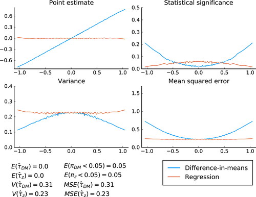
Focusing on the point estimates, we see that the OLS estimator is approximately conditionally unbiased. That is, regardless of value of $\mathbf{\Delta }$, the average point estimate is close to zero. The difference-in-means estimator on the other hand is conditionally biased, with point estimates being negatively biased for negative $\mathbf{\Delta }$ and positively biased for positive $\mathbf{\Delta }$. As we know should be the case, the unconditional expectations of the estimators are both exactly zero for each sample.

Turning to the size of the tests, we first note that the unconditional size is correct for both estimators. The conditional test is wildly off for the difference-in-means estimator (a simple t-test). The more $\mathbf{\Delta }$ deviates from zero, the higher the rejection rate of the null hypothesis. Importantly, because the test has correct size on average, the size of the test conditional on $\mathbf{\Delta }$ being close to zero is smaller than 0.05, meaning the test in that range is conservative. It is also noteworthy that for no value of $\mathbf{\Delta }$ is the difference-in-means estimator conditionally unbiased with correct size of the hypothesis test. For the conditional test for the OLS estimator, we also see that it is a little bit off from correct size, but less so than for the difference-in-means estimator. As we show in the supplementary material, this is the case for this specific sample, but over random sampling, the test size for the OLS is conditionally correct regardless of value of $\mathbf{\Delta }$.

The final two graphs show the conditional variance and MSE. Because the OLS estimator—but not the difference-in-means estimator—is approximately conditionally unbiased, these are approximately the same for the former but not the latter. The theoretical variances are given in Equations (2)(2) $$V_{{\mathcal{W}}_{\mathbf{\Delta }}}({\widehat{\tau }}_{\text{DM}})=V_{{\mathcal{W}}_{\mathbf{\Delta }}}({\overline{\epsilon }}_1-{\overline{\epsilon }}_0).$$(2) and (3)(3) $$V_{{\mathcal{W}}_{\mathbf{\Delta }}}({\widehat{\tau }}_z)=\frac{V_{{\mathcal{W}}_{\mathbf{\Delta }}}({\overline{\epsilon }}_1-{\overline{\epsilon }}_0)}{{\left(1-M_{\mathbf{\Delta }}/(n-1)\right)}^2}.$$(3) . The figure shows that $V_{{\mathcal{W}}_{\mathbf{\Delta }}}({\overline{\epsilon }}_1-{\overline{\epsilon }}_0)$ is decreasing as the magnitude of $\mathbf{\Delta }$ increases. The reason is that as $\mathbf{\Delta }$ increases, the assignment vectors become more similar to each other, and so ${\overline{\epsilon }}_1-{\overline{\epsilon }}_0$ become more similar. This result is in line with the theoretical result when the covariate is a dummy variable derived in the supplementary material. For the OLS estimator, on the other hand, the term ${\left(1-M_{\mathbf{\Delta }}/(n-1)\right)}^{-2}$ counteracts the effect of ${\overline{\epsilon }}_1-{\overline{\epsilon }}_0$ becoming more similar and the conditional variance, if anything, is increasing in the magnitude of $\mathbf{\Delta }$. Consistent with the theoretical analysis, the conditional variance is identical between the two estimators when $\mathbf{\Delta }=\mathbf{0}$. The MSE is consistently greater for the difference-in-means estimator than the OLS estimator.

Since we showed the result for a single sample of n = 20, it is natural to ask whether Figure 1 shows a general pattern or something specific to this particular sample. In the supplementary materials, we show that the same pattern emerges if we average the results over 1000 random samples.

4 Selection of Covariates

In situations when the number of observations are much larger than the number of relevant covariates ($n\gg K$), the preceding analysis suggests that it is always better to condition on the covariates than not condition on them as it will lead to a lower mean squared error and correct conditional inference. Even if a covariate is not relevant (β = 0), little is lost with a large sample size. However, if K is not order of magnitudes smaller than n, Equation (4)(4) $$\begin{array}{c}\mathit{\beta }\prime \mathbf{\Delta }{\mathbf{\Delta }}^{\prime }\mathit{\beta }+2{\mathbf{\Delta }}^{\prime }\mathit{\beta }{E}_{{\mathcal{W}}_{\mathbf{\Delta }}}({\overline{\epsilon }}_1-{\overline{\epsilon }}_0)\\ \hspace{1em}>E_{{\mathcal{W}}_{\mathbf{\Delta }}}\left({({\overline{\epsilon }}_1-{\overline{\epsilon }}_0)}^2\right)\left(\frac{1}{{\left(1-M_{\mathbf{\Delta }}/(n-1)\right)}^2}-1\right).\end{array}$$(4) implies that there is a tradeoff between adding more covariates as the bias term (${\mathbf{\Delta }}^{\prime }\mathit{\beta }$) decreases while the variance increases due to an increase in the Mahalanobis distance, $M_{\mathbf{\Delta }}$. In the extreme case, with K > n, it is not even possible to condition on all covariates in a regression. So what should one do in such a case?

A common practice is to condition only on covariates which show large imbalances, but as Mutz, Pemantle, and Pham (2019) show, such an approach will lead to incorrect inference. Another possibility would be to choose covariates based on perceived importance in explaining the outcome. However, unless such an approach is specified in a pre-analysis plan, it opens up the possibility for the researcher to select covariates in a large number of ways, potentially leading to issues such as data snooping and p-hacking. Even when the researcher is completely honest, such an approach lack transparency, making it difficult for the research community at large to ascertain the credibility of the results.

It is therefore useful to have a rule-based system of covariate selection which limits the degrees of freedom of the researcher. We propose such a rule of covariate selection which builds on the idea of randomization inference. Randomization inference after covariate adjustments is conditional on a set of assignment vectors, ${\mathcal{W}}_{\mathbf{\Delta }}$, for which $\mathbf{\Delta }=\mathbf{c}$. If this set is too small, then randomization-based justification for inference collapses (Cox 2009) and inference can only be justified under the assumption of random sampling from some population. The smallest p-value which can be attained from Fisher’s exact test is $1/\left|{\mathcal{W}}_{\mathbf{\Delta }}\right|$, so, for example, if it should be possible to achieve a p-value of 0.01 or smaller, it must be the case that there are at least 100 assignment vectors which has the same value of $\mathbf{\Delta }$. If there are a few discrete covariates, then this would generally be true. However, if the covariates are continuous, then it would typically be the case that $\left|{\mathcal{W}}_{\mathbf{\Delta }}\right|=1$ and, strictly speaking, inference based on the OLS estimator cannot be justified based on randomization.

Instead, we suggest basing inference on the set ${\mathcal{W}}_{\tilde{\mathbf{\Delta }}}$ where all elements in the set yield a distance which is approximately equal to $\mathbf{\Delta }$. Note that, asymptotically, it is the case that $M_{\mathbf{\Delta }}\sim {\chi }^2(K)$. Let ${\mathbf{\Delta }}_j:=\mathbf{\Delta }({\mathbf{W}}_j)-\mathbf{\Delta }(\mathbf{W})$, where W is the assignment vector actually chosen and ${\mathbf{W}}_j\in \mathcal{W}$. It is the case that $M_{{\mathbf{\Delta }}_j}:=\frac{n_0{n}_1}{n}{\mathbf{\Delta }}_j^{\prime }{\mathbf{\Sigma }}_{\mathbf{ZZ}}{}^{-1}{\mathbf{\Delta }}_j$ follows a noncentral chi-square distribution with K degrees of freedom and noncentrality parameter of $M_{\mathbf{\Delta }}$. We can now define the set ${\mathcal{W}}_{\tilde{\mathbf{\Delta }}}$ as ${\mathcal{W}}_{\tilde{\mathbf{\Delta }}}=\{\mathbf{W}\in \mathcal{W}:M_{{\mathbf{\Delta }}_j}\le \overline{\delta }\}$, where $\overline{\delta }$ is a small threshold value which should be set close to zero. For $\overline{\delta }=0$, it is the case that ${\mathcal{W}}_{\tilde{\mathbf{\Delta }}}={\mathcal{W}}_{\mathbf{\Delta }}$.

Let $H=\left|{\mathcal{W}}_{\tilde{\mathbf{\Delta }}}\right|$ be the number of assignment vectors with small enough distance from the original treatment assignment to approximately justify randomization-based inference. In practice, for moderately sized n it is not possible to go through all the $n_A=\left(\begin{array}{c}n\\ n_1\end{array}\right)$ assignment vectors to find H. However, by using the fact that $M_{{\mathbf{\Delta }}_j}$ follows a noncentral chi-square distribution, we can calculate the approximate size of the set as$$n_{\overline{\delta }}=F_{K,M_{\mathbf{\Delta }}}(\overline{\delta })·n_A,$$where $F_{K,M_{\mathbf{\Delta }}}(·)$ is the cdf of the noncentral chi-square distribution with K degrees of freedom and noncentrality parameter of $M_{\mathbf{\Delta }}$. If it is the case that $n_{\overline{\delta }}\ge H$, then the OLS estimator of the treatment effect, controlling for Z, can be justified from a randomization inference perspective. In practice, if $\overline{\delta }$ is small and K is reasonably large, it will be the case that $n_{\overline{\delta }}<H$. It is therefore necessary to somehow restrict the number of covariates that will be conditioned on.

We propose to condition on the principal components of Z. There are two reasons for this proposal: First, if covariates are correlated, it is a natural way of reducing the dimensionality of the covariate space. Second, principal components are naturally ordered in descending variances. Let ${\mathbf{Z}}_p^{pc}=\left[\begin{array}{cccc}{\mathbf{z}}_1^{pc}& {\mathbf{z}}_2^{pc}& \cdots & {\mathbf{z}}_p^{pc}\end{array}\right]$ be a matrix of the first p principal components of Z and ${\mathbf{\Sigma }}_{\mathbf{ZZ}}{}_p^{pc}$ be the corresponding covariance matrix; it is the case that $M_{\mathbf{\Delta }}^{pc}=\frac{n_0{n}_1}{n}{\mathbf{\Delta }}^{pc\prime }{\mathbf{\Sigma }}_{\mathbf{ZZ}}{{}_p^{pc}}^{-1}{\mathbf{\Delta }}^{pc}\sim {\chi }^2(p)$, resulting in $M_{{\mathbf{\Delta }}_j}^{pc}$ following a noncentral chi-square distribution with p degrees of freedom and noncentrality parameter of $M_{\mathbf{\Delta }}^{pc}$.

With the natural ordering of the principal components, we suggest a simple algorithm (Algorithm 1) which yield the number of principal components to condition on in a regression estimation of the treatment effect. After the components have been selected, we get the treatment effect estimator from a regression of Y on the treatment indicator, controlling for the p principal components.

Algorithm 1 Component selection

1: Set $\overline{\delta }$ and H

2: $p\leftarrow 0$

3: $n_{\overline{\delta }}\leftarrow n_A$

4: while $n_{\overline{\delta }}\ge H$ do

5: Select first p + 1 principal components and calculate the Mahalanobis distance

6: Calculate $n_{\overline{\delta }}$

7: if $n_{\overline{\delta }}\ge H$ then $p\leftarrow p+1$

8: end if

9: end while

10: return p

4.1 Simulation Results

To study how our algorithm compares to other estimators, we perform a simple simulation study. Specifically, we generate data as$$Y_i(0)=Y_i(1)={\mathbf{z}}_i\mathbf{b}+u_i,$$where $\mathbf{Z}\sim N(\mathbf{0},\mathbf{I}),\mathbf{b}=\left[\begin{array}{cccc}\frac{1}{\sqrt{K}}& \frac{1}{\sqrt{K}}& \dots & \frac{1}{\sqrt{K}}\end{array}\right]\prime$ and $u\sim N(0,1)$. With this setup, we have $\text{var}({\mathbf{z}}_i\mathbf{b})=\text{var}(u_i)$, which means the R² from a regression of $\mathbf{Y}(\mathbf{0})$ on Z should be around 0.5. For a randomly selected sample, we draw 10,000 random treatment assignment vectors and estimate the treatment effect. We then repeat this process for 1000 different samples and calculate the average MSE. For our algorithm, we let $\overline{\delta }=0.01$ and the sample size is set to n = 50 with $n_0=n_1=25$. We vary K (the number of covariates) from 2 to 40 in steps of 2.

With this setup, the covariates are orthogonal to each other in the population, and so we should not expect the PCA to effectively reduce the dimensionality of the data. Hence, this setup can be considered a “worst case” for our method. To study what happens when covariates are correlated, we use the method suggested by Lewandowski, Kurowicka, and Joe (2009) to generate correlated covariates with the parameter η being set to one.

We contrast our estimator with three other estimators: (a) the difference-in-means estimator, (b) the OLS estimator when all covariates are used as controls and (c) the cross-estimation estimator suggested by Wager, Taylor, and Tibshirani (2016). The latter estimator uses high-dimensional regression adjustments with an elastic net to select important covariates when there are many covariates relative to the number of observations.

Figure 2(a) shows the result from the simulations. Beginning with the left graph—which shows the results from orthogonal covariates—we see that with few covariates, the MSE of the difference-in-means estimator is around double that of the OLS estimator, which is what we should expect for $n\gg K$ as the covariates account for 50% of the variation in Y(0) (see, for instance, Morgan and Rubin 2012). Notably, the OLS estimator and our PCA-based estimator is identical in that case. The reason is simply that with so few covariates, all principal components are selected, and conditioning on all principal components is equivalent to conditioning on all covariates. The cross-estimation estimator lies somewhere between the difference-in-means estimator and the other estimators.

Fig. 2 MSE with homogeneous treatment effect. For each value of K, 1000 samples are drawn with 10,000 assignment vectors selected for each sample. For the cross-estimation estimator, for computational time purposes, only 100 assignment vectors are selected for each sample. The sample size is set to 50 with an equal number of treated and control units and τ = 0.

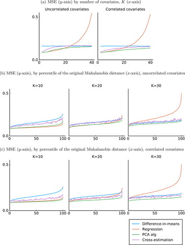
As K increases, the MSE of the difference-in-means estimator is naturally unchanged, while the MSE of the three other estimators increases. For an interval with K between 10 and 20, the OLS estimator marginally outperforms our estimator, but once the number of covariates increases further, the MSE of the OLS estimator skyrockets. For our estimator, the MSE increases slowly and stays consistently lower than that of the difference-in-means estimator. The cross-estimation estimator is clearly better than the OLS estimator for large K, but performs worse than our estimator.

The left graph shows the results from the worst-case for our estimator. In the right graph, we show results when covariates are correlated. The difference-in-means and OLS estimators are very similar to the previous case, but now our estimator outperforms both of them for all values of K (except for small K when the OLS estimator and our estimator are equivalent). The cross-estimation estimator also outperforms the other estimators for large K, but still performs worse than our estimator.

The results in Figure 2(a) shows the average of the MSE for each value of K. However, as we discussed previously, the MSE will depend on $\mathbf{\Delta }$. Because $\mathbf{\Delta }$ is K-dimensional, it is not possible to illustrate the results as we did in Figure 1. Instead, for each sample, we take the average MSE of each percentile of the Mahalanobis distance, $M_{\mathbf{\Delta }}$, and then take the average for each percentile over all 1000 samples. We show the results for K = 10, 20, 30.

Results are shown in Figure 2(b) for uncorrelated covariates and Figure 2(c) for the correlated covariates. In Figure 1, the MSE displayed a U-shaped pattern with minimum when $\mathbf{\Delta }=0$. Because the Mahalanobis distance is a (weighted) square of $\mathbf{\Delta }$, the MSE is now increasing in the Mahalanobis distance for all four estimators. We see that the MSE of the difference-in-means estimator, our PCA estimator and the cross-estimation estimator all increase at roughly the same pace, while the OLS estimator has an MSE that increases sharply for large distances once K is large. Note that the cross-estimation estimator is more variable because, for computational time purposes, we only selected 100 instead of 10,000 random assignment vectors per random sample. Also, note that this estimator works best when it can be believed that most of the covariates are uninformative, a case we do not consider here.

In Table 1 we show the size of a two-sided test of τ = 0 for each of the four estimators (5% significance level) for K = 10, 20, 30. The first column shows the average size (independent of the Mahalanobis distance). As can be seen, the difference-in-means estimator, the OLS estimator and our PCA estimator all have approximately correct size, whereas the cross-estimation estimator overrejects the null, with a rejection rate of around 8% instead of 5%.

Table 1 Size, homogeneous effects.

Quintiles	All	First	Second	Third	Fourth	Fifth
	Uncorrelated covariates
K = 10
Difference-in-means	0.05	0.023	0.036	0.047	0.06	0.085
Cross-estimation	0.08	0.053	0.067	0.073	0.09	0.116
Regression	0.05	0.05	0.05	0.05	0.05	0.05
PCA alg	0.051	0.044	0.047	0.05	0.053	0.064
K = 20
Difference-in-means	0.05	0.032	0.042	0.049	0.057	0.07
Cross-estimation	0.082	0.058	0.072	0.079	0.089	0.111
Regression	0.05	0.05	0.05	0.05	0.05	0.05
PCA alg	0.051	0.038	0.045	0.05	0.056	0.066
K = 30
Difference-in-means	0.05	0.038	0.045	0.05	0.055	0.062
Cross-estimation	0.08	0.064	0.072	0.08	0.085	0.1
Regression	0.05	0.05	0.05	0.05	0.05	0.05
PCA alg	0.051	0.041	0.047	0.051	0.055	0.061
	Correlated covariates
K = 10
Difference-in-means	0.05	0.025	0.036	0.047	0.059	0.083
Cross-estimation	0.076	0.056	0.064	0.073	0.084	0.101
Regression	0.05	0.05	0.05	0.05	0.05	0.05
PCA alg	0.051	0.049	0.05	0.05	0.051	0.053
K = 20
Difference-in-means	0.05	0.032	0.042	0.049	0.057	0.07
Cross-estimation	0.079	0.061	0.071	0.079	0.086	0.101
Regression	0.05	0.05	0.05	0.05	0.05	0.05
PCA alg	0.051	0.044	0.048	0.051	0.054	0.06
K = 30
Difference-in-means	0.05	0.038	0.045	0.05	0.055	0.062
Cross-estimation	0.082	0.068	0.079	0.081	0.084	0.097
Regression	0.05	0.05	0.05	0.05	0.05	0.05
PCA alg	0.051	0.044	0.048	0.051	0.054	0.058

NOTE: The table shows the size of a two-sided test of τ = 0 at 5% significance level. The first column shows the unconditional size, whereas the next five shows the size for each quintile of the Mahalanobis distance, $M_{\mathbf{\Delta }}$. For each value of K, 1000 samples are drawn with 10,000 assignment vectors selected for each sample. For the cross-estimation estimator, for computational time purposes, only 100 assignment vectors are selected for each sample. The sample size is set to 50 with an equal number of treated and control units. For the regression-based estimators, the standard OLS covariance matrix is used.

The following columns show the results separately for each quintile of the Mahalanobis distance, $M_{\mathbf{\Delta }}$. We now see that only the OLS estimator maintains correct size regardless of the value of the Mahalanobis distance, whereas the difference-in-means estimator clearly underrejects for small values of the Mahalanobis distance and overrejects for large values. This pattern is expected, as the difference-in-means estimator does not take the covariate imbalance into account. A similar pattern is found for the cross-estimation estimator, but with a higher rejection rate. Finally, for our PCA estimator, the rejection rate is also increasing with the Mahalanobis distance, but at a slower pace, as the covariate imbalance is partially taken into account by the selected principal components.

Finally, Table 2 shows the power of the different estimators with τ set to one (from a two-sided test of τ = 0). The results are very similar to the result for the MSE: with K = 10, the OLS estimator is the most powerful estimator, closely followed by our PCA estimator. For larger K, the OLS estimator performs much worse, while the PCA estimator continuous to perform well. The cross-estimation estimator also performs comparatively well for K = 30, but it should be noted that the power is not size-adjusted.

Table 2 Power, homogeneous effects.

Quintiles	All	First	Second	Third	Fourth	Fifth
	Uncorrelated covariates
K = 10
Difference-in-means	0.686	0.709	0.695	0.686	0.677	0.664
Cross-estimation	0.792	0.815	0.802	0.797	0.781	0.768
Regression	0.858	0.899	0.881	0.865	0.845	0.801
PCA alg	0.839	0.882	0.862	0.843	0.823	0.785
K = 20
Difference-in-means	0.686	0.701	0.691	0.686	0.68	0.673
Cross-estimation	0.74	0.759	0.744	0.741	0.737	0.72
Regression	0.744	0.831	0.788	0.753	0.713	0.635
PCA alg	0.759	0.797	0.773	0.758	0.743	0.72
K = 30
Difference-in-means	0.689	0.699	0.692	0.688	0.685	0.681
Cross-estimation	0.734	0.745	0.743	0.732	0.728	0.72
Regression	0.545	0.682	0.604	0.55	0.493	0.398
PCA alg	0.724	0.75	0.733	0.723	0.714	0.7
	Correlated covariates
K = 10
Difference-in-means	0.698	0.717	0.705	0.698	0.69	0.678
Cross-estimation	0.838	0.854	0.84	0.839	0.837	0.818
Regression	0.865	0.905	0.888	0.872	0.852	0.808
PCA alg	0.882	0.91	0.896	0.885	0.872	0.846
K = 20
Difference-in-means	0.691	0.703	0.695	0.691	0.686	0.679
Cross-estimation	0.801	0.816	0.807	0.797	0.797	0.788
Regression	0.732	0.82	0.776	0.742	0.701	0.622
PCA alg	0.82	0.85	0.832	0.821	0.808	0.787
K = 30
Difference-in-means	0.684	0.692	0.687	0.684	0.68	0.676
Cross-estimation	0.769	0.781	0.774	0.766	0.766	0.757
Regression	0.526	0.661	0.584	0.53	0.473	0.381
PCA alg	0.779	0.802	0.787	0.778	0.769	0.757

NOTE: The table shows the power from of a two-sided test of τ = 0 at 5% significance level, with τ = 1. The first column shows the unconditional power, whereas the next five shows the power for each quintile of the Mahalanobis distance, $M_{\mathbf{\Delta }}$. For each value of K, 1000 samples are drawn with 10,000 assignment vectors selected for each sample. For the cross-estimation estimator, for computational time purposes, only 100 assignment vectors are selected for each sample. The sample size is set to 50 with an equal number of treated and control units. For the regression-based estimators, the standard OLS covariance matrix is used.

Overall, we conclude that our PCA-based estimator generally outperforms the other three estimator in terms of MSE. While the size is not always correct conditional on observed differences in covariates, the issue is smaller than for the difference-in-means estimator or cross-estimation estimator. It is also important to note that when $n\gg K$, our estimator essentially collapses to the OLS estimator.

4.2 Variations of Algorithm 1

The algorithm that we suggest using is agnostic in terms of the importance of the different covariates and we therefore propose to condition on the principal components rather than the original covariates. However, in some settings the experimenter may have a priori knowledge which suggests that one or several covariates are likely to affect the outcome. In that case, it is inefficient to balance only on the principal components, and since there is no guarantee that the relevant covariate(s) are balanced with the algorithm, there can be conditional bias.

In such cases, we suggest augmenting Algorithm 1 in the following way: First the experimenter decides on the G covariates they believe are important in predicting the outcome. These covariates are in turn ranked in descending order according to their perceived importance. Then principal component analysis is performed on the remaining K – G covariates and the principal components are, just as before, ranked in descending order in terms of variance. Algorithm 1 is then performed in order of perceived importance of the covariates. If the algorithm has not terminated after the G important covariates have been selected, then the algorithm continuous with the principal components.

This augmented algorithm shares some similarities with the idea of rerandomization in tiers proposed by Morgan and Rubin (2015). The difference is that just as with regular rerandomization (Morgan and Rubin 2012), rerandomization in tiers is performed in the design phase and requires access to covariates at that time. Our algorithm is instead used after the experiment is carried out in the analysis phase.

This fact means that our algorithm could be used for data snooping and p-hacking if the experimenter decides which covariates are important only after looking at the result and, potentially, choosing to use the covariates that lead to statistically significant results of the treatment effects. Obviously, such behavior would lead to incorrect inference. Without a pre-analysis plan, researchers conducting experiments will have to argue for the particular choices they made in the analysis phase and it is up to the research community at large to decide whether these choices are justified.

With a pre-analysis plan, these concerns can be mitigated. If covariates are observed in the design phase, different rerandomization strategies are attractive options. However, in many cases, covariates may not be available in the design phase and are instead collected during the experiments (of course, by covariates in this context, we do not mean variables that can be affected by the experiment). Furthermore, in sequential experiments (such as in many clinical trials), it is not straightforward to use rerandomization. In such cases, a transparent and efficient option would be to write in the pre-analysis plan that our algorithm will be used and specify the variables that will be included, as well as the values of $\overline{\delta }$ and H that will be used. In such cases, the issues with p-hacking will be handled with, while at the same time, data will be used efficiently.

Algorithm 1 builds on the idea that the Mahalanobis distance follows a chi-square distribution (in the left-tail for values smaller than $\overline{\delta }$). Asymptotically, this is true, but it might not hold for small samples, especially with data that are far from being normal (e.g., skewed data containing outliers) and when $\overline{\delta }$ is very close to zero. Note that for very small samples (such as n < 30), no distributional approximation is needed as it would be possible to go through all treatment assignments to find all assignment vectors who fulfill the criterium in Algorithm 1. For larger samples sizes, this is not possible. However, an experimenter who, because of the sample size and data, believes that the Mahalanobis distance is unlikely to follow a chi-square distribution can simply randomly choose a large (but computationally feasible) number of assignment vectors, n_v (such as $n_v=1,000,000,000$). $n_{\overline{\delta }}$ can then be estimated in step 6 in the algorithm. This is done by taking the number of assignment vectors out of the n_v which fulfill the criteria of the Mahalanobis distance being smaller than $\overline{\delta }$ and multiply with $n_A/n_v$. For $n_A\gg n_v$ the algorithm will then likely lead to a conservative number of components.

5 Heterogeneous Treatment Effects

We now turn to the study of heterogeneous treatment effects. To do so, we consider the following two linear projections:$$\begin{array}{c}{Y}_i(0)={\alpha }_0+{\mathbf{z}}_i^{\prime }{\mathit{\beta }}_0+{\epsilon }_{0i}\\ Y_i(1)={\alpha }_1+{\mathbf{z}}_i^{\prime }{\mathit{\beta }}_1+{\epsilon }_{1i},\end{array}$$

with the estimand of interest—the sample average treatment effect—being$$\tau =\frac{1}{n}\sum _{i=1}^n(Y_i(1)-Y_i(0))={\alpha }_1-{\alpha }_0+\overline{\mathbf{z}}\prime ({\mathit{\beta }}_1-{\mathit{\beta }}_0),$$as ${\overline{\epsilon }}_0={\overline{\epsilon }}_1=0$ by construction. By demeaning the linear projections and interacting with the treatment indicator, W_i , we can write the observed outcome as(5) $$Y_i={\alpha }_0^{*}+({\mathbf{z}}_i-\overline{\mathbf{z}})\prime {\mathit{\beta }}_0+W_i\tau +W_i({\mathbf{z}}_i-\overline{\mathbf{z}})\prime \mathit{\rho }+{\eta }_i,$$(5) where ${\alpha }_0^{*}={\alpha }_0+\overline{\mathbf{z}}\prime {\mathit{\beta }}_0$, ${\eta }_i={\epsilon }_{0i}+W_i({\epsilon }_{1i}-{\epsilon }_{0i})$ and $\mathit{\rho }=({\mathit{\beta }}_1-{\mathit{\beta }}_0)$. The difference-in-means estimator can be written as$${\widehat{\tau }}_{\text{DM}}={\overline{Y}}_1-{\overline{Y}}_0=\tau +{\mathbf{\Delta }}^{\prime }\mathit{\zeta }+{\overline{\epsilon }}_{11}-{\overline{\epsilon }}_{00},$$ where $\mathit{\zeta }=\frac{n_1}{n}{\mathit{\beta }}_0+\frac{n_0}{n}{\mathit{\beta }}_1$ and ${\overline{\epsilon }}_{11}$ and ${\overline{\epsilon }}_{00}$ are the respective averages of ${\epsilon }_1$ and ${\epsilon }_0$ in the treatment and control groups. Analogous to the case with homogeneous treatment effects, we have$$E_{{\mathcal{W}}_{\mathbf{\Delta }}}({\widehat{\tau }}_{\text{DM}})=\tau +{\mathbf{\Delta }}^{\prime }\mathit{\zeta }+E_{{\mathcal{W}}_{\mathbf{\Delta }}}({\overline{\epsilon }}_{11}-{\overline{\epsilon }}_{00}).$$

Once again, we have conditional bias in the difference-in-means estimator for $\mathbf{\Delta }\ne \mathbf{0}$. Naturally, the conditional variance of the difference-in-means estimator is$$V_{{\mathcal{W}}_{\mathbf{\Delta }}}({\widehat{\tau }}_{\text{DM}})=V_{{\mathcal{W}}_{\mathbf{\Delta }}}({\overline{\epsilon }}_{11}-{\overline{\epsilon }}_{00})$$

When it comes to the OLS estimator, Equation (5)(5) $$Y_i={\alpha }_0^{*}+({\mathbf{z}}_i-\overline{\mathbf{z}})\prime {\mathit{\beta }}_0+W_i\tau +W_i({\mathbf{z}}_i-\overline{\mathbf{z}})\prime \mathit{\rho }+{\eta }_i,$$(5) suggests that to properly deal with the case of heterogeneous treatment effects, all covariates should be demeaned and included both by themselves as well as interacted with the treatment indicator. The coefficient in front of the treatment indicator by itself is then an estimator for τ. We can include all the control variables, including interactions in a $n\times 2K$ matrix $\mathbf{X}=\left[\begin{array}{cc}\tilde{\mathbf{Z}}& \mathbf{Q}\end{array}\right]$ with the ith row equaling ${\mathbf{x}}_i=\left[\begin{array}{cc}{\mathbf{z}}_i-\overline{\mathbf{z}}& ({\mathbf{z}}_i-\overline{\mathbf{z}})W_i\end{array}\right]$. In the supplementary materials we show that the OLS estimator of τ, ${\widehat{\tau }}_x$, can then be written as$${\widehat{\tau }}_x=\tau +\frac{{\overline{\epsilon }}_{11}-{\overline{\epsilon }}_{00}-\frac{1}{n-1}\mathbf{\Delta }\prime f(\mathbf{Z}\prime \mathit{\eta },{\mathbf{\Sigma }}_{\mathbf{XX}})}{1-{\tilde{M}}_{\mathbf{\Delta }}/(n-1)},$$where ${\tilde{M}}_{\mathbf{\Delta }}$ is a weighted Mahalanobis distance of $\mathbf{\Delta }$ (technically, it is the Mahalanobis distance of ${\overline{\mathbf{x}}}_1-{\overline{\mathbf{x}}}_0$) and ${\mathbf{\Sigma }}_{XX}$ is the covariance matrix of X. The difference from the case with homogeneous treatment effects is that the conditional bias of the OLS estimator no longer depends solely on ${\overline{\epsilon }}_{11}-{\overline{\epsilon }}_{00}$, but also on $\mathbf{\Delta }\prime f(\mathbf{Z}\prime \mathit{\eta },{\mathbf{\Sigma }}_{\mathbf{XX}})$; in the homogeneous case, $\mathbf{Z}\prime \mathrm{\epsilon }=\mathbf{0}$, whereas in the heterogeneous case, $\mathbf{Z}\prime \mathit{\eta }\ne \mathbf{0}$. The only time this second term disappears is when $\mathbf{\Delta }=\mathbf{0}$.

The conditional bias of the OLS estimator depends on both ${\overline{\epsilon }}_{11}-{\overline{\epsilon }}_{00}$ and $\mathbf{Z}\prime \mathit{\eta }$. The difference in bias between the difference-in-means estimator and the OLS estimator is that the former has the extra bias term ${\mathbf{\Delta }}^{\prime }\mathit{\zeta }$, whereas the latter has the extra bias term that is a function of $\mathbf{Z}\prime \mathit{\eta }$. For reasonably large sample sizes, it will in general be the case that the latter term is quite small and the difference-in-means estimator will have a greater conditional bias than the OLS estimator.

When it comes to comparing the MSE of the two estimators, the explicit expression for the OLS estimator is more complicated due to the covariance between ${\overline{\epsilon }}_{11}-{\overline{\epsilon }}_{00}$ and $\mathbf{Z}\prime \mathit{\eta }$. However, the general lesson from the case with homogeneous treatment effects still apply: if the covariates are informative, the conditional MSE of the OLS estimator will tend to be lower compared to the difference-in-means estimator. However, because covariates are also interacted with the treatment indicator, relatively fewer covariates can be included before the MSE of the OLS estimator gets larger than the difference-in-means estimator, something that is shown in the simulation results below.

The analysis here complements the findings in Freedman (2008), who discusses the extent to which randomization justifies regression adjustment in the Neyman model (Splawa-Neyman, Dabrowska, and Speed 1990). He studies the asymptotic properties when the number of units in the experiment goes to infinity and shows (a) that the OLS covariate adjustment estimator is, in general, (unconditionally) biased (of order $1/n$), (b) that the conventional OLS estimated standard errors estimator are inconsistent, and (c) that, with unbalanced designs, the OLS estimator also could be (unconditionally) less efficient than the difference-in-means estimator asymptotically. However, Lin (2013) shows (a) that the Eicker-Huber-White standard error estimator (Eicker 1967; Huber 1967; White 1980) is consistent or asymptotically conservative and (c) that the OLS estimator from Equation (5)(5) $$Y_i={\alpha }_0^{*}+({\mathbf{z}}_i-\overline{\mathbf{z}})\prime {\mathit{\beta }}_0+W_i\tau +W_i({\mathbf{z}}_i-\overline{\mathbf{z}})\prime \mathit{\rho }+{\eta }_i,$$(5) is, asymptotically, at least as (unconditionally) efficient as the difference-in-means estimator.

To study the conditional inference in the presence of heterogeneous treatment effects, we next show results from a simulation study.

5.1 Simulation Results with Heterogeneous Treatment Effects

To study the properties of the estimators with heterogeneous treatment effects in a simulation study, we generate data as$$\begin{array}{c}{Y}_i(0)={\mathbf{z}}_i\mathbf{b}+u_{0i},\\ Y_i(1)={\mathbf{z}}_i\mathbf{b}+\gamma +u_{1i}.\end{array}$$where $\mathbf{Z}\sim N(\mathbf{0},\mathbf{I}),\mathbf{b}=\left[\begin{array}{cccc}\frac{1}{\sqrt{K}}& \frac{1}{\sqrt{K}}& \dots & \frac{1}{\sqrt{K}}\end{array}\right]$ and both u₀ and u₁ following standard normal distributions. In these simulations, the heterogeneity therefore comes solely from the differing errors. As before, for our algorithm, we let $\overline{\delta }=0.01$ and the sample size is set to n = 50 with $n_0=n_1=25$. Because we can use up to 2K covariates in a regression (because of the interactions), we vary K from 2 to 20 in steps of 1. $n_{\overline{\delta }}$ in Algorithm 1 is now initiated at $n_A/2$.

The Eicker-Huber-White estimator can be severely downward biased in small samples. A large number of estimators adjusting for this small sample bias for the inference to the population has been suggested in the literature (MacKinnon 2013). The so-called HC2 and HC3 covariance estimators are in general considered better estimators in small samples when the data suffers from a high degrees of heteroscedasticity. In our setting, heteroscedasticity is limited. Thus, we follow the procedure suggested in Lin (2013) and use the Eicker-Huber-White estimator.

Overall, with heterogeneous treatment effects, the MSE of the different estimators exhibits similar patterns to those shown in Figure 2 for homogeneous treatment effects, with the difference that our PCA estimator always perform as good or better than the OLS estimator. The results corresponding to Figure 2 are shown in the supplementary materials.

Table 3 shows the size of a test where the null is set to the sample average treatment effect at 5% significance level. We now see that no estimator gives correct size, with the difference-in-means, OLS and PCA estimators all typically being conservative, while the cross-estimation estimator continuous to overreject. However, the average size-distortion is in general quite small. Conditional on the Mahalanobis distance, the same pattern as before is present: as the Mahalanobis distance increases, the rejection rate for all estimators increase. Different from the case with homogeneous treatment effects, this is true also for the OLS estimator.

Table 3 Size, heterogeneous effects.

Quintiles	All	First	Second	Third	Fourth	Fifth
	Uncorrelated covariates
K = 5
Difference-in-means	0.039	0.014	0.023	0.033	0.047	0.08
Cross-estimation	0.058	0.038	0.046	0.053	0.063	0.088
Regression	0.038	0.035	0.036	0.037	0.039	0.042
PCA alg	0.038	0.035	0.036	0.037	0.039	0.042
K = 10
Difference-in-means	0.04	0.02	0.029	0.037	0.046	0.066
Cross-estimation	0.063	0.044	0.051	0.06	0.068	0.091
Regression	0.044	0.04	0.042	0.044	0.046	0.05
PCA alg	0.043	0.036	0.039	0.041	0.045	0.053
K = 15
Difference-in-means	0.039	0.023	0.032	0.038	0.045	0.059
Cross-estimation	0.068	0.047	0.059	0.066	0.076	0.093
Regression	0.052	0.047	0.05	0.052	0.054	0.058
PCA alg	0.044	0.034	0.039	0.043	0.047	0.057
	Correlated covariates
K = 5
Difference-in-means	0.039	0.016	0.023	0.033	0.046	0.077
Cross-estimation	0.054	0.039	0.044	0.051	0.061	0.075
Regression	0.038	0.035	0.036	0.037	0.039	0.042
PCA alg	0.037	0.034	0.036	0.037	0.039	0.041
K = 10
Difference-in-means	0.039	0.02	0.029	0.036	0.046	0.065
Cross-estimation	0.059	0.044	0.051	0.053	0.065	0.08
Regression	0.044	0.039	0.042	0.044	0.046	0.05
PCA alg	0.041	0.037	0.04	0.041	0.042	0.046
K = 15
Difference-in-means	0.039	0.024	0.031	0.038	0.045	0.058
Cross-estimation	0.066	0.047	0.057	0.063	0.073	0.088
Regression	0.052	0.046	0.049	0.052	0.054	0.057
PCA alg	0.042	0.037	0.04	0.041	0.044	0.049

NOTE: The table shows the size of a test where the null is the sample average treatment effect at 5% significance level. The first column shows the unconditional size, whereas the next five shows the size for each quintile of the Mahalanobis distance, $M_{\mathbf{\Delta }}$. For each value of K, 1000 samples are drawn with 10,000 assignment vectors selected for each sample. For the cross-estimation estimator, for computational time purposes, only 100 assignment vectors are Cselected for each sample. The sample size is set to 50 with an equal number of treated and control units. For the regression-based estimators, the Eicker-Huber-White robust covariance matrix is used.

Finally, Table 4 shows the result corresponding to Table 2 in the homogeneous case. Because we are interested in studying power, the null is now set to zero instead of the sample average treatment effect. The PCA estimator generally outperforms the other three estimators on average, as well as conditionally for small Mahalanobis distances. The cross-estimation estimator is generally slightly more powerful for large distances and roughly equally powerful for K = 15. However, this can partly be attributed to the fact that the test rejects the null slightly too often.

Table 4 Power, heterogeneous effects.

Quintiles	All	First	Second	Third	Fourth	Fifth
	Correlated covariates
K = 5
Difference-in-means	0.588	0.599	0.594	0.589	0.583	0.575
Cross-estimation	0.711	0.722	0.718	0.716	0.707	0.695
Regression	0.748	0.782	0.768	0.754	0.737	0.698
PCA alg	0.748	0.782	0.768	0.754	0.737	0.698
K = 10
Difference-in-means	0.589	0.597	0.592	0.589	0.585	0.58
Cross-estimation	0.674	0.683	0.681	0.68	0.666	0.659
Regression	0.667	0.733	0.7	0.674	0.644	0.587
PCA alg	0.68	0.729	0.702	0.682	0.661	0.625
K = 15
Difference-in-means	0.588	0.594	0.59	0.588	0.585	0.582
Cross-estimation	0.65	0.66	0.652	0.647	0.65	0.639
Regression	0.537	0.631	0.577	0.541	0.501	0.435
PCA alg	0.64	0.678	0.655	0.64	0.624	0.601
	Correlated covariates
K = 5
Difference-in-means	0.592	0.6	0.596	0.593	0.589	0.583
Cross-estimation	0.742	0.755	0.75	0.745	0.738	0.723
Regression	0.753	0.787	0.772	0.76	0.742	0.703
PCA alg	0.757	0.788	0.774	0.763	0.747	0.712
K = 10
Difference-in-means	0.601	0.608	0.604	0.602	0.599	0.594
Cross-estimation	0.703	0.716	0.708	0.705	0.698	0.688
Regression	0.673	0.737	0.706	0.68	0.65	0.593
PCA alg	0.716	0.754	0.734	0.719	0.702	0.672
K = 15
Difference-in-means	0.597	0.603	0.6	0.597	0.595	0.591
Cross-estimation	0.683	0.691	0.69	0.68	0.677	0.675
Regression	0.537	0.632	0.578	0.541	0.501	0.434
PCA alg	0.691	0.726	0.706	0.692	0.678	0.654

NOTE: The table shows the power from of a test of τ = 0 at 5% significance level, with γ = 1. The first column shows the unconditional power, whereas the next five shows the power for each quintile of the Mahalanobis distance, $M_{\mathbf{\Delta }}$. For each value of K, 1000 samples are drawn with 10,000 assignment vectors selected for each sample. For the cross-estimation estimator, for computational time purposes, only 100 assignment vectors are selected for each sample. The sample size is set to 50 with an equal number of treated and control units. For the regression-based estimators, the Eicker-Huber-White robust covariance matrix is used.

Overall, the conclusions from the simulations on homogeneous treatment effects carry over to the heterogeneous case. We find that the PCA estimator generally performs the best by having the smallest MSE and highest power, while being slightly conservative in terms of test size.

6 Concluding Discussion

Randomized controlled trials are considered the gold standard for causal inferences as randomization of treatment guarantees that the difference-in-means estimator is an unbiased estimator of the average treatment effect under no model assumption. However, this unbiasedness only holds under randomization over all possible assignment vectors.

Indeed, in this article we show that conditional on observed imbalances in covariates, the difference-in-means estimator is in general biased, with associated statistical tests having incorrect size. As researchers are generally encouraged to investigate whether covariates are balanced, this fact puts the practitioner in an awkward position: on the one hand, the estimator is unbiased over all possible randomizations; on the other hand, conditional on the differences actually observed, the estimator is most likely biased.

A solution to this problem is to condition on observed covariates in a regression model, and we show that the OLS estimator is approximately conditionally unbiased. On the other hand, Athey and Imbens (2017) cautions against the use of the OLS estimator in analyzing randomized experiments as the OLS estimator was not developed with randomization inference in mind, resulting in a disconnect between the assumptions needed for regression and for randomized controlled trials. Specifically, they write that “it is easy for the researcher using regression methods to go beyond analyses that are justified by randomization, and end up with analyses that rely on a difficult-to-assess mix of randomization assumptions, modeling assumptions, and large sample approximations.” Similarly, Freedman (2008) writes that “Regression adjustments are often made to experimental data. Since randomization does not justify the models, almost anything can happen.”

Furthermore—and as discussed in Mutz, Pemantle, and Pham (2019)—if practitioners adjust for covariates only when they are imbalanced between treatment and control groups, the inference will be compromised. A further problem also discussed in Mutz, Pemantle, and Pham (2019) is that with many covariates, many different regression estimators are possible raising the concern of p-hacking. With these objections in mind—and with the need to avoid adding all covariates in the regression model to avoid a high MSE—we develop an algorithm based on the principal components of the covariates and select only so many principal components that can be justified based on randomization inference, thereby alleviating the concerns raised by Athey and Imbens (2017), Freedman (2008), and Mutz, Pemantle, and Pham (2019).

To be fair, also this algorithm can be used for data snooping, by for example, adding or removing covariates making up the principal components or by choosing different thresholds used in the algorithm in determining the number of assignment vectors. The bottom line is that without a pre-analysis plan, there is always an open door for data snooping by fraudulent researchers.

A better strategy is instead to use efficient experimental designs together with a pre-analysis plan. With continuous covariates the Mahalanobis-based rerandomization strategies of Morgan and Rubin (2012) and Morgan and Rubin (2015) are options in reducing the conditional bias ex-ante. If the experimental design is published in a pre-analysis plan, this will prevent p-hacking and data snooping. However, data on covariates may not be available in the design phase, making it impossible to use rerandomization strategies. In such a case, an attractive option would be to commit to using the algorithm developed in this article already in the pre-analysis plan. The algorithm can either be used completely agnostically (i.e., without using any information about importance of covariates) or, as discussed in Section 4.2, it can be used together with prior information about covariate importance. By committing to using the algorithm, data can be used efficiently, while at the same time the transparency and credibility of the RCT can be maintained.

Acknowledgments

We are grateful for comments and suggestions from seminar participants at IFAU, Peking University, Stockholm University, and Umeå University.

Supplementary Materials

The supplementary materials contain mathematical derivations and some additional simulation results. Replication code for all simulation results is available at https://github.com/mattiasnordin/Conditional-inference-in-experiments.

References

- Athey, S., and Imbens, G. W. (2017), “The Econometrics of Randomized Experiments,” in Handbook of Economic Field Experiments, volume 1 of Handbook of Field Experiments, eds. A. V. Banerjee and E. Duflo, pp. 73–140. Amsterdam: North-Holland.
- Cox, D. R. (2009), “Randomization in the Design of Experiments,” International Statistical Review, 77, 415–429. DOI: 10.1111/j.1751-5823.2009.00084.x.
- Deaton, A., and Cartwright, N. (2018), “Understanding and Misunderstanding Randomized Controlled Trials,” Social Science & Medicine, 210, 2–21. DOI: 10.1016/j.socscimed.2017.12.005.
- Eicker, F. (1967), “Limit Theorems for Regressions with Unequal and Dependent Errors,” in Proceedings of the Fifth Berkeley Symposium on Mathematical Statistics and Probability (Vol. I), pp. 59–82. University California Press, Berkeley, CA.
- Freedman, D. (2008), “On Regression Adjustments to Experimental Data,” Advances in Applied Mathematics, 40, 180–193. DOI: 10.1016/j.aam.2006.12.003.
- Huber, P. J. (1967), “The Behavior of Maximum Likelihood Estimates Under Nonstandard Conditions,” in Proceedings of the Fifth Berkeley Symposium on Mathematical Statistics and Probability (Vol. I), pp. 221–233. Berkeley, CA: University California Press.
- Lewandowski, D., Kurowicka, D., and Joe, H. (2009), “Generating Random Correlation Matrices Based on Vines and Extended Onion Method,” Journal of Multivariate Analysis, 100, 1989–2001. DOI: 10.1016/j.jmva.2009.04.008.
- Lin, W. (2013), “Agnostic Notes on Regression Adjustments to Experimental Data: Reexamining Freedman’s Critique,” The Annals of Applied Statistics, 7, 295–318. DOI: 10.1214/12-AOAS583.
- MacKinnon, J. G. (2013), “Thirty Years of Heteroskedasticity-Robust Inference,” in Recent Advances and Future Directions in Causality, Prediction, and Specification Analysis: Essays in Honor of Halbert L. White Jr., eds. X. Chen and N. R. Swanson, pp. 437–461. New York: Springer.
- Miratrix, L. W., Sekhon, J. S., and Yu, B. (2013), “Adjusting Treatment Effect Estimates by Post-stratification in Randomized Experiments,” Journal of the Royal Statistical Society, Series B, 75, 369–396. DOI: 10.1111/j.1467-9868.2012.01048.x.
- Morgan, K. L., and Rubin, D. B. (2012), “Rerandomization to Improve Covariate Balance in Experiments,” The Annals of Statistics, 40, 1263–1282. DOI: 10.1214/12-AOS1008.
- Morgan, K. L., and Rubin, D. B (2015), “Rerandomization to Balance Tiers of Covariates,” Journal of the American Statistical Association, 110, 1412–1421.
- Mutz, D. C., Pemantle, R., and Pham, P. (2019), “The Perils of Balance Testing in Experimental Design: Messy Analyses of Clean Data,” The American Statistician, 73, 32–42. DOI: 10.1080/00031305.2017.1322143.
- Splawa-Neyman, J., Dabrowska, D. M., and Speed, T. P. (1990), “On the Application of Probability Theory to Agricultural Experiments. Essay on Principles. Section 9,” Statistical Science, 5, 465–472. DOI: 10.1214/ss/1177012031.
- Wager, S., Du, W., Taylor, J., and Tibshirani, R. J. (2016), “High-Dimensional Regression Adjustments in Randomized Experiments,” Proceedings of the National Academy of Sciences, 113, 12673–12678. DOI: 10.1073/pnas.1614732113.
- White, H. (1980), “Using Least Squares to Approximate Unknown Regression Functions,” International Economic Review, 21, 149–170. DOI: 10.2307/2526245.