The Wald Confidence Interval for a Binomial p as an Illuminating “Bad” Example

Abstract

When teaching we usually not only demonstrate/discuss how a certain method works, but, not less important, why it works. In contrast, the Wald confidence interval for a binomial p constitutes an excellent example of a case where we might be interested in why a method does not work. It has been in use for many years and, sadly enough, it is still to be found in many textbooks in mathematical statistics/statistics. The reasons for not using this interval are plentiful and this fact gives us a good opportunity to discuss all of its deficiencies and draw conclusions which are of more general interest. We will mostly use already known results and bring them together in a manner appropriate to the teaching situation. The main purpose of this article is to show how to stimulate students to take a more critical view of simplifications and approximations. We primarily aim for master’s students who previously have been confronted with the Wilson (score) interval, but parts of the presentation may as well be suitable for bachelor’s students.

KEYWORDS:

• Correlation
• Coverage probability
• Score statistic
• Skewness
• Wald statistic

1 Introduction

Student: “I have computed a 95% confidence interval for p, but I don’t get the same endpoints as when using the software package. I have checked it several times.”

Teacher: “I am sure you haven’t done anything wrong. The interval in the course book is actually never used in practice, but, anyway, it’s easy to compute!”

We will not reveal the ambitious student’s reaction to this reply $\dots$

The standard two-sided Wald interval for the binomial p is by now well known to be of low quality with respect to actual coverage and it ought to be stricken from all courses in mathematical statistics/statistics as the recommended interval to use. However, it still lingers on in quite a few textbooks. For those still in doubt about its dubious properties, Brown, Cai, and DasGupta (2001, 2002) and Andersson (2022) are recommended reading. Should we then forget about this interval altogether and focus only on preferred alternatives, such as the Wilson (1927), also known as the score, and the Agresti and Coull (1998) intervals? Well, perhaps not. The Wald interval in its construction and behavior actually constitutes a very good “bad” example of what can happen if you only strive for simplicity, while completely ignoring possible negative consequences. The interval itself (1) $$\widehat{p}\pm \frac{z}{\sqrt{n}}\sqrt{\widehat{p}(1-\widehat{p})},$$(1) where $\widehat{p}=x/n$, x is the observed value of $X\sim \text{Bin}(n,p)$ and z is the $1-\alpha /2$ quantile of the standard normal distribution, is surely appealing to students in its simplicity, and, over the years, generations of them have been able to memorize it and probably some of them still remember it. The present and forthcoming generations may also be confronted with this interval, but now for a different purpose.

Problems concerning intervals constructed from Wald statistics also arise, for instance, in the cases of the difference between two binomial proportions and the mean of a Poisson distribution. See, for example, Agresti and Caffo (2000) and Andersson (2015), respectively. Especially the latter situation offers to the students, as a possible added exercise, a natural comparison with our present case.

Even if there is a vast amount of published papers in high quality journals which highlight the deficiencies of the Wald interval, the treatment of this estimation problem in textbooks is quite varied. For instance, in Larsen and Marx (1981), the Wilson interval is derived followed by the comment, “In practice though, all terms in $z_{\alpha /2}^2$ are usually dropped—on the grounds that $z_{\alpha /2}$ will be quite small relative to n.” This dropping of terms means that we will, in fact, obtain the Wald interval. In the fourth edition of this book from 2006, there is no longer any mention of the Wilson interval and concerning the assumption of approximate normality of the Wald statistic, it is stated that, “$\dots$ a result that seems plausible given that X/n is the maximum likelihood estimator for p.” The classic Hogg, McKean, and Craig (2005) is another example of a textbook which only brings up the Wald interval. In Casella and Berger (2002), there is a discussion involving both the Wald and Wilson intervals, but the criticism of the Wald interval does not go beyond, “Wald procedures produce intervals that are just too short for small n, with the Wald interval also suffering from endpoint maladies.” At this stage it may be pointed out that even in Lehmann (1999) there are only a few hints on the deficiencies of the Wald interval that will be examined in this article. It can further be mentioned that in the textbook currently used by the author for teaching undergraduate statistics students, only the Wald interval is brought up for the estimation of the binomial p, and quite misleadingly, the authors have chosen to demonstrate its behavior for p = 0.5. Moreover, they combine this with n = 35, thereby obtaining one of the “lucky pairs” highlighted in Brown, Cai, and DasGupta (2001), meaning one of the few combinations of n and p = 0.5, for which the Wald interval actually works well. However, there are also examples of textbooks entirely abandoning the Wald interval. As noted in Agresti and Caffo (2000), soon after the publication of Agresti and Coull (1998), the confidence interval suggested in that article was brought up in Samuels and Witmer (1999) and McClave and Sincich (2000). Navidi (2006) also uses the Agresti-Coull interval, remarking about the Wald interval, “Recent research shows that the interval can be improved by modifying both n and $\widehat{p}$ slightly.”

Although some individual technical details and results can be found elsewhere in the literature, the approach in this article is centered on teaching mathematical statistics for bachelor’s and master’s students. We will describe a possible way to improve the students’ understanding of approximations based on asymptotic arguments, in general, and why the Wilson confidence interval is much better behaved than the Wald’s, in particular. A key factor as to why the Wald interval is badly behaved is that the point estimator and its standard error are correlated. To the best of the author’s knowledge, this is not recognized in influential papers and textbooks, some of which are previously mentioned.

The article is organized as follows. In Section 2, we present the Wald and score statistics and show how they are related, and we further point out the extent to which the distribution of the Wald statistic deviates from the normal. The cases $\widehat{p}=0$ and 1 are also discussed. Section 3 deals with explicit results, especially concerning coverage and noncoverage behavior of both types of intervals, but also briefly comments on the issue of interval lengths. The article ends with conclusions and comments about what to make of these findings in the classroom.

2 The Wald and Score Statistics and Their Corresponding Intervals

We will start with the origin of the Wald interval, namely, the Wald statistic (2) $$\frac{\sqrt{n}(\widehat{p}-p)}{\sqrt{\widehat{p}(1-\widehat{p})}}$$(2) and then ask the students about what could be the problem with this expression, bearing in mind that we hope for approximate normality in distribution. From the author’s experience, a common reply is, that the estimated p’s in the denominator could cause trouble and rightly so, although all the negative implications will surely not be clear at this stage. What the students have learned previously is that for $X\sim \text{Bin}(n,p)$ it holds that $X\stackrel{\text{appr}}{\sim }N(np,np(1-p))$, if $np(1-p)>10$. Other qualifications also appear in the literature.

This is equivalent to saying that (3) $$\frac{\sqrt{n}(\widehat{p}-p)}{\sqrt{p(1-p)}}\stackrel{\text{appr}}{\sim }N(0,1),$$(3) which is actually a result for the score statistic usually taught for hypothesis testing and the starting point for the Wilson interval. At this point, the students should find the Fisher information number $I_n(p)=n/[p(1-p)]$ for X and verify that the expression in (3) is obtained by using the general definition of the score statistic $$\frac{\frac{\partial }{\partial p}\log \hspace{0.17em}{f}_X(x|p)}{\sqrt{I_n(p)}}.$$

Likewise, the expression (2) is obtained by the observed information number ${\widehat{I}}_n(\widehat{p})=n/[\widehat{p}(1-\widehat{p})]$. Now, (3) implies that (4) $$\begin{array}{c}P\left(\left|\frac{\sqrt{n}(\widehat{p}-p)}{\sqrt{p(1-p)}}\right|\le z\right)\approx 1-\alpha \\ \hspace{1em}\iff P\left(\widehat{p}-\frac{z}{\sqrt{n}}\sqrt{p(1-p)}\le p\le \widehat{p}+\frac{z}{\sqrt{n}}\sqrt{p(1-p)}\right)\\ \hspace{1em}\approx 1-\alpha .\end{array}$$(4)

The next step, regrettably often found in textbooks, is to further claim that (5) $$P\left(\widehat{p}-\frac{z}{\sqrt{n}}\sqrt{\widehat{p}(1-\widehat{p})}\le p\le \widehat{p}+\frac{z}{\sqrt{n}}\sqrt{\widehat{p}(1-\widehat{p})}\right)\approx 1-\alpha .$$(5)

From this we arrive at the Wald interval (1). Of course, the interval (1) can be obtained directly from the Wald statistic (2) under the assumption of approximate normality, see below. However, to assume that there is nothing problematic about moving from (4) to (5) is completely wrong, as we will see. We could also simply argue, that replacing p by $\widehat{p}$ in the denominator of the score statistic (3) could seriously affect the validity of the approximate normality.

So, how are the Wald and score statistics related? We first observe that the Wald statistic (2) is linear in p, but nonlinear in $\widehat{p}$ and that the reverse is true for the score statistic in (3). Besides, we can write (6) $$\frac{\sqrt{n}(\widehat{p}-p)}{\sqrt{\widehat{p}(1-\widehat{p})}}=\frac{\sqrt{n}(\widehat{p}-p)}{\sqrt{p(1-p)}} \sqrt{\frac{p(1-p)}{\widehat{p}(1-\widehat{p})}}$$(6) and argue that the left-hand side converges in distribution to N(0, 1), since the score statistic converges in distribution to N(0, 1) according to the Central Limit Theorem, and the second factor on the right-hand side converges in probability to 1. This may be a task for the students to clarify using a Slutsky argument. So, in the limit, everything seems fine, but what about the “real world” situation with a fixed finite n? The students should at this stage be reminded of the t-statistic $\sqrt{n}(\overline{X}-\mu )/S$, for which the numerator and the denominator are independent under the assumption of $X\sim N(\mu ,{\sigma }^2)$. In our case, on the other hand, $\widehat{p}$ and $\widehat{p}(1-\widehat{p})$ seem indeed correlated. Now, a good exercise is to show that (7) $$\text{cov}\left(\widehat{p},\frac{\widehat{p}(1-\widehat{p})}{n-1}\right)=\frac{p(1-p)(1-2p)}{n^2} .$$(7)

Naturally, the factor $1-2p$ is the most interesting part of this expression as it determines whether the correlation is positive (p < 1∕2), zero (p = 1/2) or negative (p > 1∕2). Not surprisingly, the “best” case occurs when p = 1/2 and symmetry holds for the binomial distribution. See also Andersson (2022). Another question now arises: What are the consequences of this correlation?

To answer the posed questions, let us first exemplify with n = 50 and p = 0.25, for which we will compare the distributions of the Wald and score statistics. From a probability plot the students will observe what appears to be negative bias and skewness for the Wald statistic. Table 1 summarizes measures of moments and the values for the Wald statistic clearly fail to approximate those for the standardized normal distribution. In this respect, the score statistic is much better behaved with only a slight positive skewness. Beforehand, one might have thought that the main, or possibly only, issue of the Wald statistic is an increase in variance when compared with the score statistic, but this is apparently not the case. The change from slight positive skewness for the score statistic to more substantial negative skewness for the Wald statistic is due to the covariance (7) and, in particular, the factor $1-2p$, which for this case is positive. The students are further encouraged to study the effects of other combinations of n and p, for instance, smaller n and p > 0.5.

Table 1 Bias, variance, skewness and kurtosis for the standardized normal random variable, the score statistic and the Wald statistic (approximate values) when n = 50 and p = 0.25.

	bias	variance	skewness	kurtosis
St. normal	0	1	0	3
Wald	–0.090	1.1	–0.48	4.0
Score	0	1	0.16	3.0

NOTE: For a random variable X with expected value μ and variance ${\sigma }^2$ skewness is defined as $E[{(X-\mu )}^3]/{\sigma }^3$ and kurtosis as $E[{(X-\mu )}^4]/{\sigma }^4$. If $X\sim \text{Bin}(n,p)$, skewness and kurtosis are $(1-2p)/\sqrt{np(1-p)}$ and $3+[1-6p(1-p)]/[np(1-p)]$, respectively. Since these quantitites are unitless, the score statistic shares these expressions with the binomial X. The approximate values of variance, skewness and kurtosis for the Wald statistic are found in Table 2 on p. 167 in Brown et al. (2002).

In the probability plot for the Wald statistic, $\widehat{p}=0$ and $\widehat{p}=1$ are naturally excluded, since for these outcomes the Wald statistic is not real-valued and therefore, formally speaking, no moments exist. Some students may have commented previously on the fact that the Wald interval is actually not an interval for these cases and here they are faced with another anomaly, which however, will be ignored in the following.

We now want to, at least approximately, quantify the bias of (6). Therefore, we first make a Taylor linearization of $\sqrt{p(1-p)/[\widehat{p}(1-\widehat{p})]}$ around $\widehat{p}=p$ and get $$\begin{array}{c}\frac{\sqrt{n}(\widehat{p}-p)}{\sqrt{\widehat{p}(1-\widehat{p})}}\approx \frac{\sqrt{n}(\widehat{p}-p)}{\sqrt{p(1-p)}}\left[1-\frac{1-2p}{2p(1-p)}(\widehat{p}-p)\right]\\ =\frac{\sqrt{n}(\widehat{p}-p)}{\sqrt{p(1-p)}}-\frac{\sqrt{n}(1-2p)}{2{(p(1-p))}^{3/2}}{(\widehat{p}-p)}^2.\end{array}$$

Noting that $E[{(\widehat{p}-p)}^2]=V(\widehat{p})=p(1-p)/n$, the students are now able to arrive at the approximation $$E\left(\frac{\sqrt{n}(\widehat{p}-p)}{\sqrt{\widehat{p}(1-\widehat{p})}}\right)\approx -\frac{1-2p}{2\sqrt{np(1-p)}}.$$

Thus, the factor $1-2p$ plays an important part also for the bias. It can further be noted that if this expression is used for n = 50 and p = 0.25, the approximation for the bias is –0.082. The value –0.090 in Table 1 is obtained from a Taylor expansion of higher order. See expression (2.1) on p. 166 in Brown et al. (2002). Now, a discussion naturally leads to a statistic adjusting for the approximate bias: $$\frac{\sqrt{n}(\widehat{p}-p)}{\sqrt{\widehat{p}(1-\widehat{p})}}+\frac{1-2p}{2\sqrt{np(1-p)}}.$$

Estimating the second term by plugging in $\widehat{p}$, the students can work out that the resulting adjusted confidence interval is $$\widehat{p}+\frac{1-2\widehat{p}}{2n}\pm z\sqrt{\frac{\widehat{p}(1-\widehat{p})}{n}}.$$

This can be shown to be an improvement of the original Wald interval in terms of coverage, but, bias adjusted or not, the Wald procedure suffers from an inability to produce an interval when $\widehat{p}=0$ or 1. This naturally leads to a discussion about what one can do about these outcomes. For example, x = 0 leads to [0, 0], which the students will agree, is both absurd and completely noninformative. At least two options are available and the first is simply to look at what the Wilson interval, derived from (3) by solving for p in a quadratic equation, (8) $$\frac{\widehat{p}+\frac{z^2}{2n}\pm \frac{z}{\sqrt{n}}\sqrt{\widehat{p}(1-\widehat{p})+\frac{z^2}{4n}}}{1+\frac{z^2}{n}}$$(8) will yield when $\widehat{p}$ is 0 or 1. It is to be noted that the score statistic in (3) is well-defined for all possible values of $\widehat{p}$. It is a simple exercise to figure out that the resulting intervals when $\widehat{p}=0$ and $\widehat{p}=1$ are $(0,z^2/(z^2+n))$ and $(n/(z^2+n),1)$, respectively. The students may then toy with different values of z and n to get some numerical feeling for these bounds. A question may come up whether these bounds are really reliable and this leads us to the second option, which involves exact calculation using the binomial distribution. We (or rather the students) solve for p in ${(1-p)}^n=\alpha$ and $p^n=\alpha$, to get an upper and lower bound, respectively, for one-sided confidence intervals with exact confidence level $1-\alpha$. $P(X=0)={(1-p)}^n$, which is a decreasing function of p and $P(X=n)=p^n$, which is an increasing function of p. See also Bickel and Doksum (1977) and Louis (1981). We can then check numerically that the Wilson bounds are quite accurate, that is, that $z^2/(z^2+n)\approx 1-{\alpha }^{1/n}$. At this point, if not earlier, the students might wonder why we do not in general simply use the binomial distribution without relying on the normal approximation for the purpose of constructing by test inversion a confidence interval for p. The short answer would be that the resulting interval, known as the Clopper-Pearson’s, is known to be quite conservative, while also suffering from extended length.

3 Coverage and Noncoverage Properties and Expected Lengths of the Wald and Wilson Intervals

Now it is time to check the corresponding coverage probabilities and the students may choose their own method to accomplish this. Probably many will prefer the option of simulating values of X and compute relative frequencies of coverage, in other words Monte Carlo simulation, since this has become close to default for investigations concerning properties of statistics in general. This can of course be done with high precision given today’s computer capacity, but why depend on simulations when one can do exact computations? Straightforwardly, for a given combination of n and p and for each outcome x, we simply compute the interval of interest and investigate whether it covers p or not. Summing up the binomial probabilities corresponding to intervals which include p then gives us the coverage probability. So, you just have to emphasize to the students that for given p, the distribution of X is known. Actually, the students can do it both ways and thereby be able to check directly the accuracy of their simulation results.

The results in Table 2 give some hints as to the performances of the Wald and Wilson intervals, but the poor quality of the Wald interval is not really clear from this investigation only. Moreover, the monotonic behavior of both intervals in terms of coverage, one increasing in p, the other decreasing, seems suspiciously simple. We need more evidence and this may come from the natural extension of computing the coverage for, say, 999 equidistant values of $p:$ $0.001,\dots ,0.999$ and then plotting the coverages in one graph. Now, is this grid of points fine enough to capture all possible fluctuations and spikes? Wang (2007) provides a result which enables exact calculation of the confidence coefficient (the infimum of the coverage probabilities). From Example 1 in that paper, we find that the confidence coefficient for the Wilson interval when n = 50 is 0.8376. This is to be compared with the corresponding minimum of coverage probabilities in our computations, which is 0.8605. If we instead use values of p from 0.0001 to 0.9999, the minimum coverage probability is 0.8395, attained for p = 0.0035. This is still not the same value as in Wang (2007), because the presented p = 0.0035 in that paper is a rounded number. So, if you want to find the variation of coverage probabilities in extreme detail, a very fine grid is indeed needed. For the purpose of comparison between the Wald and the Wilson interval, though, the first choice of grid is considered to be sufficient. Again, letting n = 50, we clearly see the difference in performance in favor of the Wilson interval in Figure 1. Related to the previous discussion, the confidence coefficient is 0 for the Wald interval. Naturally, the ragged performances of both intervals, although somewhat less pronounced for the Wilson interval, are due to the lattice structure of the binomial distribution. This is investigated in detail in Brown et al. (2002). Of course, the students should test other values of n, like n = 5, which is a case for which no one would dare to use the Wald interval, but where the Wilson interval is certainly no disaster. Brown et al. (2001) highlighted the useless/misleading qualifications found in the literature regarding sufficient values of n for using the Wald interval, such as “n quite large”!

Fig. 1 Coverage probabilities for the Wald and Wilson intervals when n = 50 and $\alpha =0.05$.

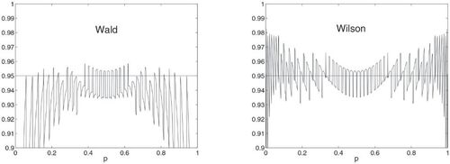
Table 2 Coverage probabilities for the Wald and Wilson intervals when n = 50, $p=0.1, 0.3$, and 0.5 and $\alpha =0.05$

	p = 0.1	p = 0.3	$p=0.5$
Wald	0.8789	0.9347	0.9351
Wilson	0.9703	0.9567	0.9351

Are we then through with the dissection of the Wald interval in particular? No! We will return to the negative effects of biased and skewed statistics and now concentrate on noncoverage probabilities. We usually say that the Wald interval is an approximate $100(1-\alpha )\%$ symmetric confidence interval for p. However, we have seen here that the coverage is often far lower than the nominal level, but what about the probabilities of “missing to the left” (lower noncoverage) and “missing to the right” (upper noncoverage) of p? These should be roughly the same, and we can easily check whether this is the case by direct computation. Continuing with n = 50, the students will then be able to present the results as in Figure 2, which are quite dramatic. The lower noncoverage probability for the Wald interval is close to the nominal 2.5% only in a narrow neighborhood of p = 0.5.

Fig. 2 Lower noncoverage probabilities for the Wald and Wilson intervals when n = 50 and $\alpha =0.05$.

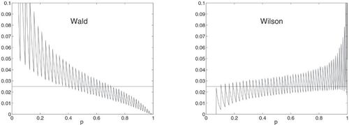
A discussion should then follow about the reasons for the displayed pattern. Therefore, we go back to the aforementioned factor $1-2p$ in the covariance expression (7). Looking at the Wilson interval again, its mid-point is (9) $$\frac{\widehat{p}+\frac{z^2}{2n}}{1+\frac{z^2}{n}} .$$(9)

Is this somehow related to $1-2\widehat{p}$ as an estimator of $1-2p$? It is certainly not clear directly that there is a simple connection, but the students may try to rewrite (9). The result, nevertheless, is that $$\frac{\widehat{p}+\frac{z^2}{2n}}{1+\frac{z^2}{n}}=\widehat{p}+\frac{z^2}{2n} \frac{1-2\widehat{p}}{1+\frac{z^2}{n}}$$

This is indeed revealing. The Wilson interval corrects the deficiency of the Wald interval so that the former is moved in the “right” direction, and this adjustment is related to both bias and skewness of the Wald statistic. This is the main reason why the Wilson interval is so much better behaved with respect to both coverage and noncoverage. At this stage, we may also discuss the consequences of nonbalanced noncoverage probabilities when dealing with one-sided intervals.

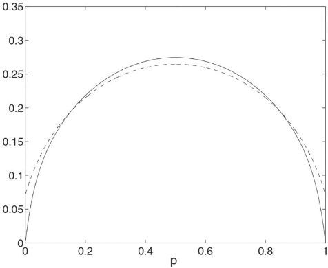
Even though we have prioritized a discussion of coverage and noncoverage probabilities, expected lengths of confidence intervals are also of interest. One would perhaps expect that, at least, the Wald interval has an advantage over Wilson’s in terms of shorter length, as was referred to in Casella and Berger (2002). But, from Figure 3, we immediately observe that this is not generally true. For n = 50, the Wilson interval has actually a shorter expected length for $0.2\le p\le 0.8$.

Fig. 3 Expected length for the Wald (solid) and Wilson (dotted) intervals when n = 50 and $\alpha =0.05$.

What we have not yet brought up as a general problem is the approximation of a discrete distribution to a continuous, which affects both the Wald and Wilson intervals. The students have probably previously seen the use of the continuity correction in the binomial case, and this issue can certainly be discussed within the present inference context as well. So, the question is, can we somewhat “save” the Wald interval?

Applying the normal approximation to $X+1/2$ instead of X leads to the “corrected” interval $$\widehat{p}+\frac{1}{2n}\pm \frac{z}{\sqrt{n}}\sqrt{\widehat{p}(1-\widehat{p})} .$$

The students can try different combinations of n and p to check the coverage for $\alpha =0.05$, for example. All in all, this is certainly not a good enough recipe for enhancing the coverage of the Wald interval and we still have the issues related to $\widehat{p}=0$ and 1. The properties of this interval are investigated in Newcombe (1998).

4 Conclusions and Comments

As mentioned, we primarily think of master’s students in mathematical statistics/statistics as the suitable target population for the estimation issues brought up in this article. An inference course at that level usually includes asymptotic results and this demonstration of the problematic Wald interval could therefore be included in a lecture containing asymptotically motivated procedures. However, most parts should be suitable also for bachelor’s students, the exceptions perhaps being details of asymptotics and the Taylor approximation. Since there are quite a few details to discuss and digest, it might be good to construct an assignment for the students to work on, for say, a week. Including some or all of the details discussed in this article, this task for the students would then primarily deal with the following issues:

• A comparison of the distributions of the Wald statistic (2) and the score statistic (3), using different combinations of n and p.

• A corresponding comparison regarding coverage and noncoverage properties and expected lengths.

After this excursion, besides learning more about the specific problem of constructing a well-behaved confidence interval for p in the binomial distribution, the students will also, hopefully, have become aware of

• the negative effects when a point estimator is correlated with its standard error.

• the fact that constructing a confidence interval which is centered around an unbiased point estimator can be far from optimal, thus, emphasizing that point and interval estimation are indeed different concepts of statistical inference.

• the fact that asymptotic results (necessary but usually not sufficient for approximations) should be interpreted with a certain amount of caution in the finite sample situation.

• the fact that rather than performing a simulation in a routine fashion, one should first check whether it is possible to do exact computations.

Acknowledgments

The author thanks three referees, an associate editor, and the editor for encouraging and helpful comments, which have substantially improved the article.

Disclosure Statement

The author reports there are no competing interests to declare.

References

- Agresti, A., and Caffo, B. (2000), “Simple and Effective Confidence Intervals for Proportions and Difference of Proportions Result from Adding Two Successes and Two Failures,” The American Statistician, 54, 280–288. DOI: 10.2307/2685779.
- Agresti, A., and Coull, B.A. (1998), “Approximate is Better than ’Exact’ for Interval Estimation of Binomial Proportions,” The American Statistician, 52, 119–126. DOI: 10.2307/2685469.
- Andersson, P. G. (2015), “A Classroom Approach to the Construction of an Approximate Confidence Interval of a Poisson Mean Using One Observation,” The American Statistician, 69, 159–164. DOI: 10.1080/00031305.2015.1056830.
- Andersson, P. G. (2022), “Approximate Confidence Intervals for a Binomial p – Once Again,” Statistical Science, 73, 598–606.
- Bickel, P. J., and Doksum, K. A. (1977), Mathematical Statistics: Basic Ideas and Selected Topics, San Francisco: Holden-Day.
- Brown, L. D., Cai, T. T., and DasGupta, A. (2001), “Interval Estimation for a Binomial Proportion,” Statistical Science, 16, 101–117. DOI: 10.1214/ss/1009213286.
- Brown, L. D., Cai, T. T., and DasGupta, A. (2002), “Confidence Intervals for a Binomial Proportion and Asymptotic Expansions,” The Annals of Statistics, 30, 160–201.
- Casella, G., and Berger, R. L. (2002), Statistical Inference (2nd ed.), Duxbury: Thomson Learning.
- Hogg, R. V., McKean, J. W., and Craig, A. T. (2005), Introduction to Mathematical Statistics (6th ed.), Pearson: Prentice Hall.
- Larsen, R. J., and Marx, M. L. (1981), An Introduction to Mathematical Statistics and its Applications, Englewood Cliffs, NJ: Prentice Hall.
- Lehmann, E. L. (1999), Elements of Large-Sample Theory, New York: Springer.
- Louis, T. A. (1981), “Confidence Intervals for a Binomial Parameter After Observing No Successes,” The American Statistician, 35, 154. DOI: 10.2307/2683985.
- McClave, J. T., and Sincich, T. (2000), Statistics (8th ed.), Englewood Cliffs, NJ: Prentice Hall.
- Navidi, W. (2006), Statistics for Engineers and Scientists, New York: McGraw–Hill.
- Newcombe, R. G. (1998), “Two-sided Confidence Intervals for the Single Proportion: Comparison of Seven Methods,” Statistics in Medicine, 17, 857–872. DOI: 10.1002/(SICI)1097-0258(19980430)17:8<857::AID-SIM777>3.0.CO;2-E.
- Samuels, M. L., and Witmer, J. W. (1999), Statistics for the Life Sciences (2nd ed.), Englewood Cliffs, NJ: Prentice Hall.
- Wang, H. (2007), “Exact Confidence Coefficents of Confidence Intervals for a Binomial Proportion,” Statistica Sinica, 17, 361–368.
- Wilson, E. B. (1927), “Probable Inference, the Law of Succession, and Statistical Inference,” Journal of the American Statistical Association, 22, 209–212. DOI: 10.1080/01621459.1927.10502953.