Hierarchical Spatio-Temporal Change-Point Detection

Abstract

Detecting change-points in multivariate settings is usually carried out by analyzing all marginals either independently, via univariate methods, or jointly, through multivariate approaches. The former discards any inherent dependencies between different marginals and the latter may suffer from domination/masking among different change-points of distinct marginals. As a remedy, we propose an approach which groups marginals with similar temporal behaviors, and then performs group-wise multivariate change-point detection. Our approach groups marginals based on hierarchical clustering using distances which adjust for inherent dependencies. Through a simulation study we show that our approach, by preventing domination/masking, significantly enhances the general performance of the employed multivariate change-point detection method. Finally, we apply our approach to two datasets: (i) Land Surface Temperature in Spain, during the years 2000–2021, and (ii) The WikiLeaks Afghan War Diary data.

KEYWORDS:

• Clustering
• Functional data
• Land surface temperature
• Multivariate analysis
• Point patterns
• Satellite images
• Trace-variogram

1 Introduction

Time series of spatial data, for example, satellite images and estimated intensity surfaces of point patterns, often face naturally/artificially emerging space-dependent distributional changes. Under what is commonly referred to as “separability” in the spatial statistical literature (Cressie and Wikle 2015), one assumes that the studied phenomenon may be described as a temporally varying rescaling of a spatial base distribution. It has, however, been well noted that separability, to a large degree, is a mathematically convenient assumption rather than an assumption reflecting the data at hand (Cressie and Wikle 2015); the observed changes often tend to appear in new/different spatial locations as time progresses. Simultaneous detection of the spatial regions and times of such changes is not only scientifically interesting in itself, but is often a crucial component for subsequent more advanced statistical analyses including model fitting, prediction, etc. As modern datasets tend to be large and complex, with frequent naturally/artificially occurring changes, the need for methods which enable detection of change-points in the distribution of (spatially referenced) time-ordered observations is steadily increasing.

Not surprisingly, change-point detection has a long history; it was first discussed to split univariate time series into homogeneous subsets in terms of the mean (Page 1954, 1955). Gradually, different methodologies, from different statistical points of view, have been developed to detect changes in various characteristics, for example, means and variances of time-ordered observations (see Horváth and Rice 2014; Aminikhanghahi and Cook 2017; Truong, Oudre, and Vayatis 2020 and the references therein). Over time, change-point detection approaches started to be applied to a range of different applications, including flood volume (Xiong et al. 2015), financial returns of stocks (Sundararajan and Pourahmadi 2018), or the normalized difference vegetation index (Moradi et al. 2022), among other contexts. Moreover, the modern-day availability of multivariate data and potential relationships between the associated marginals have highlighted the need to develop multivariate change-point detection approaches.

Discrete data, including almost all time-ordered datasets, are rarely actually discrete in nature, but in fact the outcome of a discrete sample of a continuous phenomenon, for example, a collection of functions reflecting temperature in various spatial locations. Berkes et al. (2009) and Aston and Kirch (2012) proposed different frameworks/tests to perform multivariate change-point analyses when dealing with functional data. Matteson and James (2014) developed a nonparametric approach to hierarchically detect/locate multiple change-points for multivariate time-ordered data. Liu et al. (2020) proposed a unified data-adaptive framework to detect change-points for high-dimensional data. Generally, multivariate change-point detection is performed by assuming that all marginals/series/dimensions/components undergo changes jointly. However, as the size of the data grows, this assumption might easily be violated due to internal/local dependencies between different marginals. Thus, some authors considered the case where only a sparse/dense subset of the marginals undergoes changes, while the rest of the marginals do not experience any change (Zhang et al. 2010; Wang and Samworth 2018; Hahn, Fearnhead, and Eckley 2020). In the multivariate context, a common way to treat data has usually been to first reduce the dimension to one, based on desirable aggregation techniques, and then to apply some univariate change-point detection method. For instance, Wang and Samworth (2018) proposed to aggregate/project data by a suitable projection direction and then locate change-points through CUSUM statistics for the projected series. Hahn, Fearnhead, and Eckley (2020) argued that such an approach may be computationally costly, especially when the number of components increases, and instead proposed a Bayesian approach to estimate the projection direction. Grundy, Killick, and Mihaylov (2020) noted that such approaches, which reduce the dimension to one, are generally developed to detect a change in a single parameter. Thus, they mapped a multivariate time series, by measuring distances and angles between each marginal and a reference marginal, to two dimensions, which are used to simultaneously detect changes in the mean and the variance.

With a growing number of marginals/series/dimensions/components, as previously indicated, it is more likely that there exist distinct subsets of data exhibiting unique/similar temporal behaviors. Moreover, as the length of the study period grows, the time series in question is more likely to face temporal distributional changes. Once the majority of the marginals/series/dimensions/components undergo similar changes jointly, it becomes less challenging to detect change-points. However, such an assumption might easily be violated as the number of marginals increases. With this said, in a high-dimensional/multivariate setting, one may find distinct subsets (most likely of different sizes) of marginals undergoing different types of changes at dissimilar times. Such changes may include slow/rapid deviations from the past with(out) returning to the past state, and/or abrupt changes. Multivariate change-point detection tends to be quite complicated when for example, (i) changes in several subsets of marginals act in different directions, (ii) there are subsets experiencing changes of different magnitudes, (iii) the sizes of the subsets undergoing changes are different, and (iv) the occurrence times of the changes in different subsets are close to each other. Such circumstances may easily cause domination/masking among different change-points and consequently lead to rather poor detection/precision rates; for example, when change-point methods are based on global distance measurements, aggregation, and/or global dimension reduction which may accidentally force different change-points to cancel each other out (see Section 4 for details). For practical situations where these issues occur, see Section 5. The literature has mostly focused on univariate change-point detection, and generally, in multivariate settings, assumed that either all or the majority of the marginals/series/dimensions/components undergo changes jointly. Moreover, multivariate change-point methods generally do not reveal which (subsets of the) marginals undergo changes. Thus, a treatment in connection with domination/masking between different change-points occurring in distinct subsets of the marginals is, to date, lacking in the literature.

Motivated by the above, in this article we propose an approach to find sub-regions such that, within each sub-region, marginals show similar temporal behaviors. In order to find such sub-regions, we propose the use of a weighted metric for the marginals, which enables the incorporation of potential spatial correlation between (nearby) marginals, and then hierarchically groups them into disjoint clusters. Hence, conditionally on a spatial dependence structure, we may proceed to study multivariate temporal evolution in a nonseparable fashion. Our approach locally searches for change-points within the estimated sub-regions. Under these circumstances, we prevent marginals with different temporal behaviors and change-points from being studied jointly when performing change-point analyses. Thus, domination/masking between change-points of different sub-regions tends to not happen, and consequently the rate of detection/precision increases. Through a simulation study, when employing common linkage functions in the clustering part and considering both spatially correlated and independent time series, we study various settings where different change-points may dominate/mask each other. The quality of the clustering outcome is assessed through the Rand index and a separation index, which we introduce in order to study how well we assign sub-regions with distinct change-points to different clusters. The achieved gain in change-point detection is measured through the rate of detection/precision.

Throughout, labels starting with the prefix “S” refer to items in the supplementary material of the article.

2 Multivariate Change-Point Detection

We here consider a set of locations, $z_1,\dots ,z_n\in W\subset {\mathbb{R}}^d,n\ge 1,d\ge 1$, which typically represent a set of monitoring places/sites. Next, given a time interval T, we attach a multivariate random function/process $X(t)=(X_1(t),\dots ,X_n(t)),t\in T$, to these spatial locations. It is noteworthy that the marginals $X_1,\dots ,X_n$ may be dependent which is a deviation from the classical functional data analysis setting (Ramsey and Silverman 2005). In other words, we consider dependent functional data where time is continuous and, here, we are particularly interested in the scenario where the dependence structure for the marginals is governed by their associated locations, that is, $z_1,\dots ,z_n$. Note that we may consider the decomposition (1) $$X_i(t)={\mu }_i(t)+{ϵ}_i(t),\mathrm{\hspace{1em}}\mathrm{\hspace{1em}}t\in T, 1\le i\le n,$$(1) where ${\mu }_i(t)=\mathbb{E}[X_i(t)]$ is the mean function of X_i, and ${ϵ}_i(·)$ is a zero-mean residual stochastic process with $\text{var}({ϵ}_i(·))=\text{var}(X_i(·))$. See Section S1.1, supplementary materials for technical details. It should be noted that, in practice, data are not sampled continuously in time but rather at discrete time points, that is, we sample a collection of dependent univariate time series, which will be the focus of this article. Some practical examples are given in Section S1.2.

Given an n-dimensional stochastic process $X(t)=(X_1(t),\dots ,X_n(t)),t\in T$, either in continuous or discrete time, let ${\Theta }_i(t)=({\theta }_{i,1}(t),\dots ,{\theta }_{i,q}(t)),t\in T,1\le i\le n$, correspond to $q\ge 1$ characteristics/parameters of X_i such as mean, variance, etc. In multivariate change-point detection the main interest lies in alerting when, for some i, ${\Theta }_i(t)$ undergoes changes (Aston and Kirch 2012; Matteson and James 2014; Liu et al. 2020; Grundy, Killick, and Mihaylov 2020). Formally speaking, to discover change-points $\{{\tau }_1,\dots ,{\tau }_k\}\subset T$, one deals with the null hypothesis ${\mathcal{H}}_0:$ constant distribution for all marginals over the time period T, versus the alternative hypothesis ${\mathcal{H}}_1:$ some marginals undergo changes, at times ${\tau }_1,\dots ,{\tau }_k$, in some parameters. In other words, the alternative hypothesis ${\mathcal{H}}_1$, for some ${\Theta }_i(t)$, claims different behaviors for any two consecutive time periods, separated by τ_j, $1\le j\le k$. If k = 1 the problem reduces to the detection of at most one change (AMOC). Note that, in contrast to the classical setting, we do not assume that the changes occur jointly across all marginals X_i, since, in practice, it is rarely the case that all X_i’s face changes of the same type or undergo changes at the same time. Moreover, nearby locations usually tend to experience similar changes in terms of time but possibly of different magnitudes, which might be a sign of spatial dependence. Further technical details can be found in Section S1.1.1.

Our objective here is to develop an approach to detect possible change-points in the associated marginal time series while taking the inherent multivariate (spatially governed) dependence structure into account. This allows us to borrow strength from the fact that (spatially) close marginal time series tend to have similar temporal distributional properties, which in turn may lead to having similar change-points. In addition, we may detect subsets of locations with similar change-points (in terms of time position) of (dis)similar magnitudes.

3 Hierarchical Spatio-Temporal Change-Point Detection

From a geostatistical point of view, functions corresponding to spatially nearby sites tend to have similar temporal behaviors which, in turn, makes it more likely that temporal changes happen simultaneously within a spatially restricted group of functions. For instance, temperature measurements at different weather stations over time are such that nearby stations show similar trends and changes. It is worth emphasizing that similarity between nearby functions (in space and/or time) can be the result of (spatial and/or temporal) changes in both the mean structure and the dependence structure; recall (1). Note further that a mean shift may, by pure chance, be canceled by a shift in the noise term of a process, which may lead to missing the detection of an actual change.

We argue that spatially associated multivariate change-point analyses may benefit from a refinement where we first group the univariate marginal time series into similar/spatially close groups of time series, before carrying out group-wise change-point analyses. Note that the larger the dataset, and the inherent distances, the bigger the chance that the general heterogeneity in the collection of processes/series under study is increased. In particular, there is an increased chance that different sub-regions exhibit different change-points.

We could, in principle, treat each marginal series as its own entity, meaning that we independently carry out an individual univariate analysis for each marginal series. This has a few drawbacks, most notably that we discard any inherent dependencies, which in turn may result in detected changes being labeled as changes in the characteristic of interest, for example, the mean, when in fact they do not correspond to such changes. Moreover, aside from the evident computational burden associated with such an approach, there is also no borrowing of strength taking place, that is, we do not statistically exploit that nearby functions have the same/similar marginal distributions to improve the estimation. Hereby, as has been well noted in the literature (Matteson and James 2014; Liu et al. 2020), a more sensible approach is multivariate change-point analysis, where the marginal functions are analyzed jointly. Since all marginals are handled jointly here, there is an increased chance that changes in some marginals dominate/conceal changes in some other marginals, and consequently one may not be able to detect all existing changes. Note that the domination/concealment may clearly depend on, for example, the types of changes occurring (e.g., up-/down-ward jumps), magnitudes of the changes, and the time difference between consecutive changes. In addition, existing methods do not necessarily reveal for which specific marginal(s) a given change-point occurs.

In line with the discussion above, in Definition 1, we present a general approach to hierarchically carry out change-point detection by first grouping the univariate marginal time series into similar/spatially close groups and then, conditionally on the group associations, carrying out multivariate change-point detection. Our approach may be viewed as a middle-ground between multivariate and univariate approaches, both conceptually and computationally.

Definition 1

(Hierarchical spatio-temporal change-point detection). Consider the multivariate time series $x(t)=(x_1(t),\dots ,x_n(t))$, $t\in T$, resulting from a discrete-time sampling of an n-dimensional continuous-time stochastic process X, which is attached to a set of spatial locations $z_1,\dots ,z_n\in W\subset {\mathbb{R}}^d,d\ge 1,n\ge 2$. Further, consider a suitable clustering approach based on (a discrete-time approximation of) a functional distance $d(·,·)$ and a linkage function. Given a chosen multivariate change-point method, any method which detects change-points of the multivariate time series in accordance with Algorithm 1 is referred to as a hierarchical spatio-temporal change-point detection (HSTCPD) method.

Algorithm 1:

Hierarchical spatio-temporal change-point detection

Input:

A (discrete-time approximation of a) functionaldistance $d(·,·)$ which takes the (spatial)dependence/correlation among the functions into account;

A linkage function;

An index $\alpha (·)$ to find optimal clusters;

A multivariate change-point detection method;

Data:

A multivariate time series $x(t)=(x_1(t),\dots ,x_n(t)),t\in T,n\ge 2$, with associated spatial locations $z_1,\dots ,z_n\in W\subset {\mathbb{R}}^d,d\ge 1$;

Result:

Disjoint subsets ${\mathcal{C}}_j\subset \{1,\dots ,n\}$ with associated spatial locations $\{z_i:i\in {\mathcal{C}}_j\}$ and a set of change-points ${\mathcal{T}}_j\subset T,j=1,\dots ,r,1<r<n$;

Generate a dendrogram for x based on the chosen metric and linkage function;

Given the dendrogram and the chosen metric, find $r=\text{arg} {\max }_{r\prime =2,\dots ,n}\alpha (r\prime )$;

Let ${\mathcal{C}}_1,\dots ,{\mathcal{C}}_r$ denote the clusters associated to r;for $j=1,\dots ,r$ do

Apply the multivariate change-point detection method to $\{x_i(t):t\in T\},i\in {\mathcal{C}}_j$;

Denote the resulting change-points by ${\mathcal{T}}_j$, where

${\mathcal{T}}_j=\varnothing$ if no change-point is found and

${\mathcal{T}}_j=\{{\tau }_{1,j},\dots ,{\tau }_{k_j,j}\},k_j\ge 1$, otherwise;end

Note that, in Definition 1, since one can employ any well-established multivariate change-point detection method, the statistical/mathematical properties of the chosen change-point methodology will still be met. Nevertheless, the only difference comes from the fact that here the chosen methodology will be independently applied to disjoint subsets ${\mathcal{C}}_1,\dots ,{\mathcal{C}}_r,1<r<n$, of marginals. We note that this form of clustering preserves the potential spatial dependencies while detecting the corresponding change-points. Note further that the general performance of HSTCPD tends to either that of univariate methods, if $r\to n$, or classical multivariate approaches, if $r\to 1$.

For spatially dependent data, a detailed background on suitable metrics, different linkage functions (Single, Complete, and Ward.D2) and different ways to find an optimal number of clusters (Ch, Dunn, and Dunn2) is given in Section S1.3.

4 Numerical Evaluation

This section is devoted to studying the performance of our proposal in Definition 1 under various settings. In each setting we deal with time series of 200 images, where each image contains 400 pixels within the bounding box $W={[0,1]}^2$. In other words, we consider a multivariate time series $x(t)=(x_1(t),\dots ,x_{400}(t)),t\in T=\{1,\dots ,200\}$, where the spatial locations z_i, $i=1,\dots ,400$, represent pixel locations. Throughout our simulation study, we consider two regions, hereafter called clouds, which undergo (multiple) abrupt changes in their means (and variances) at different time points. The rest of the image does not experience any distributional change. The sizes and positions of the clouds, as well as the magnitudes/types of changes, vary according to the scenarios described below.

4.1 Description of Scenarios

We first consider two general situations according to which an image time series is built. In the first situation, given a base realization in the form of a spatial Gaussian random field on W, with mean 0 and a Gaussian covariance function with scale 5 and variance 10 (given in (S5)), which we sample at the pixel locations, we generate a multivariate pixel time series by, for each $t\in T$, adding the base realization to an error/noise field where all marginals $x_i(t),i=1,\dots ,400$, come from iid standard normal distributions. This means that we consider spatial correlation but temporal conditional independence. In the second situation, identically to the error field in situation one, we consider completely independent pixel time series, where all marginals $x_i(t),i=1,\dots ,400,t=1,\dots ,200$, come from iid standard normal distributions. Now, for each such situation, we consider the following scenarios:

• Scenario I: There exist two clouds (contained within circles of radius 0.12), each corresponding to 21 pixels (5.25% of the full image of 400 pixels), where the pixel time series contained within the first cloud (${\text{cl}}_1\subset W$) experience an upward change of magnitude one while those within the second cloud (${\text{cl}}_2\subset W$) face a downward change of the same magnitude. Here, we are interested to see how our proposal can improve the state-of-the-art when different subregions undergo changes which are similar in magnitude but different in terms of direction.

  Concerning the times at which changes occur, for ${\text{cl}}_1$ we consider a change at time 60. For ${\text{cl}}_2$, which similarly has only one change, we consider different choices for the time of occurrence: $70,80,90,100,110,120$. We do this to further study the performance of our proposal when the time distance between the two change-points increases. The results for the situation where there exists spatial correlation among different pixel time series and the change-point in ${\text{cl}}_2$ occurs at time 70 are presented in the main paper, whereas the rest of the results can be found in Section S2.1.

• Scenario II: The cloud sizes are the same as in Scenario I, but here the pixel time series within ${\text{cl}}_1$ experience an upward change of magnitude one while the pixels within ${\text{cl}}_2$ face an upward change of magnitude two. Here, we are interested in analyzing the fact that changes of larger magnitudes may hide/impede/blur the detection of smaller changes. The times at which changes occur are analogous to Scenario I, and corresponding results for both situations can be found in Section S2.2.

• Scenario III: There exist two clouds that both undergo upward changes of magnitude one. Here, ${\text{cl}}_1$ includes 21 pixels, while ${\text{cl}}_2$ consists of 69 pixels (17.25% of the full image), contained within a circle of radius 0.24. The interest here is to detect different changes of the same magnitude and direction, which occur within regions of different sizes. The times at which changes occur are analogous to Scenario I, and corresponding results for both situations can be found in Section S2.3.

  In addition to the above scenarios, we consider the below two cases to further study the masking/concealment problem when there are multiple changes per each cloud ${\text{cl}}_1$ and ${\text{cl}}_2$.

• Scenario IV: Here, we only consider spatially correlated pixel time series with the cloud sizes similar to Scenario I. Further, we consider two change-points per cloud according to which ${\text{cl}}_1$ (${\text{cl}}_2$) experiences an upward (downward) change of magnitude one at time 60 (70) and a downward (upward) change of the same size at time 120 (130). Further details together with all corresponding results can be found in Section S2.6.

• Scenario V: Here, completely independent pixel time series are used with the cloud sizes similar to Scenario I. Further, we consider two change-points in the mean and the variance per cloud, where ${\text{cl}}_1$ experiences an upward change of magnitude one, in the mean, at time 60 and a change in the variance at time 120. The cloud ${\text{cl}}_2$ experiences changes of the same magnitude, at times 70 (mean) and 130 (variance), but in different directions compared to their counterparts in ${\text{cl}}_1$. Further details together with all corresponding results can be found in Section S2.7.

  Furthermore, in light of the scalability implications of our proposal, we next proceed to deliberate upon the following scenario.

• Scenario VI: Here, we replicate Scenario I using image time series of similar size to the two real data analyzed in Section 5; details and results are presented in Section S2.8.

For any combination of the aforementioned settings, scenarios, and times of changes, we simulate 200 image time series. We add that when there is no correlation between different pixels, we fix the position of the clouds, whereas in the presence of spatial correlation we let the position of the clouds vary from one simulation to another. 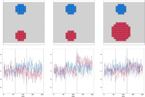More specifically, we let ${\text{cl}}_1$ and ${\text{cl}}_2$ be centered around the maximum and minimum of the generated field. For the case of no spatial correlation, Figure 1 shows the positions of the clouds within the Scenarios I–III together with examples of pixel time series for each part of the image. In the top row, the two clouds are displayed in blue and red, and the rest of the image, which is the region facing no change, is displayed in grey. The bottom row shows examples of pixel time series when a change happens at time 60 (corresponding to cloud I) and another when a change happens at time 120 (corresponding to cloud II).

Fig. 1 Top row: image representation including clouds (in red and blue) where changes occur. Bottom row: examples of pixel time series within each part of the image. Columns from left to right: Scenario I, Scenario II, Scenario III. Vertical lines represent the change-points which are 60 and 120 in this case.

4.2 Benchmarks

We evaluate the performance of the considered clustering approaches based on two indices to firstly see how well pixel time series are grouped, and second to see how well the two clouds are separated. Therefore, we first make use of the Rand index (Rand 1971) (2) $$\mathbf{RI}=\frac{TP+TN}{TP+FP+TN+FN},$$(2) where TP, the true positives, is the number of pairs of pixels that in reality belong to the same cluster, and also do so according to the clustering procedure; FP, the false positives, is the number of pairs of pixels that in reality do not belong to the same cluster, but do so according to the clustering procedure; TN, the true negatives, is the number of pairs of pixels that in reality do not belong to the same cluster, and also do not do so according to the clustering procedure; and finally FN, the false negatives, is the number of pairs of pixels that in reality belong to the same cluster, but do not do so according to the clustering procedure. The Rand index (2), which takes values between 0 and 1, is indeed a measure of similarity between any obtained classification and the ground truth data. However, in our simulation study the cluster with no change-point forms the biggest part of the image (89.5% for the first two scenarios and 77.5% for Scenario III). Thus, in situations where only one of the clouds is detected (see e.g., Figure S3) or both clouds are detected but as one unique cluster (Figure S19), the Rand index (2) may still claim a good performance. Since throughout the simulation study, one of our main aims is to have the clouds ${\text{cl}}_1$ and ${\text{cl}}_2$ in different clusters, to avoid any domination/concealment between changes, we further define the separation index (3) $$\begin{array}{c}\mathbf{S}\mathbf{I}=1-\frac{1}{2}[\frac{1}{\#{\text{cl}}_1}\sum _{i\in {\text{cl}}_1}\mathbf{1}\left\{l(i)\in \underset{j\in {\text{cl}}_2}{\cup }l(j)\right\}\\ +\frac{1}{\#{\text{cl}}_2}\sum _{j\in {\text{cl}}_2}\mathbf{1}\left\{l(j)\in \underset{i\in {\text{cl}}_1}{\cup }l(i)\right\}],\end{array}$$(3) that takes values between 0 (fully overlapped) and 1 (fully separated); here l(i) denotes the clustering procedure’s labeling of pixel i. In fact, the index SI aims at measuring how well we separate the cloud ${\text{cl}}_1$ from ${\text{cl}}_2$ by averaging the proportions of pixels in ${\text{cl}}_1$ and ${\text{cl}}_2$ which are assigned to the same cluster. This said, ideal clustering happens when both RI and SI are simultaneously equal to one. Note that (2) and (3) only measure the goodness of pre-clustering/classification. We add that, throughout our simulation studies, when employing the clustering techniques, which are presented in Section S1.3, we consider the maximum number of clusters to be 20.

4.3 Change-Point Detection Methods

With respect to change-point detection results, we compare the performance of our proposal with the general multivariate change-point detection (Classic) and a situation where we are aware of the positions of the clouds (Conditional). We do this to see how good we perform compared to the Classic approach, and also how close we can get to the ideal situation represented by Conditional. The state-of-the-art, in change-point detection, is represented by the methods of Matteson and James (2014), Liu et al. (2020), and Grundy, Killick, and Mihaylov (2020), which we have applied by means of the R package ecp (the divisive approach implemented in the function e.divisive), version 3.1.3 (James and Matteson 2015), R-code (data-adaptive test) supplied by the authors of Liu et al. (2020), and the R package changepoint.geo (the function geomcp), version 1.0.1 (Grundy 2020). For both e.divisive and geomcp we let the maximum time distance between change-points be 5. In order to study the effect of incorporating the proposed clustering on the performance of the employed change-point detection methods, we demonstrate detection rates for all detected change-points, with respect to the total number of simulations, generated by the Classic, Conditional, and HSTCPD approaches. We have relegated all results pertaining to the methods of Liu et al. (2020) and Grundy, Killick, and Mihaylov (2020) in combination with HSTCPD to Sections S2.4 and S2.5, respectively.

Note that here we are only interested in studying the performance of the considered change-point methods when domination/concealment happens between different marginals; for other types of performance analyses we refer the reader to Matteson and James (2014), Liu et al. (2020), and Grundy, Killick, and Mihaylov (2020).

4.4 Results

4.4.1 Scenario I

This scenario studies the case where ${\text{cl}}_1$ undergoes an upward change while ${\text{cl}}_2$ experiences a change of the same magnitude but in a different direction, that is, downwards. Our goal here is to see if such circumstances generally tend to mislead change-point detection methods, thus, yielding erroneous results, and further to see how HSTCPD improves the overall performance of change-point detection methods.

Table 1 shows the obtained average RI and SI, based on 200 simulations of Scenario I. One can see that the Complete and Ward.D2 linkage functions give rise to substantially lower RI than the Single linkage. This is due to the fact that the former two generally favor more compact clusters, and consequently they inflate FN, that is, the number of pairs of pixels that in reality belong to the same cluster, but do not do so according to the clustering procedure. Moreover, since these two give compact clusters, they are always able to separate the two clouds wherein change-points are placed, that is, having high SI. However, the Single linkage function generally suggests fewer clusters and thereby it is not sufficiently successful in separating the two clouds. In particular, the combination of the Single linkage function and Dunn2, to find the optimal number of clusters, seems to perform quite poorly. The joint performance of Single and Dunn is slightly better but seems to depend on the time difference between the two inserted change-points; as this difference increases, that is, as the time of change in ${\text{cl}}_2$ tends to 120, SI increases slightly. The joint performance of Single and Ch seems to be the best in this scenario since both RI and SI are high for all choices of occurrence time for ${\text{cl}}_2$.

Table 1 Scenario I with spatially correlated pixel time series. An upward change with magnitude one happens at time 60 in cl₁, whereas the time index of a downward change of the same magnitude, happening in cl₂, varies between 70 and 120. Average Rand index RI (separation index SI) are reported.

Linkage	Optimal	Change-point for ${\text{cl}}_2$
		70	80	90	100	110	120
Single	Ch	0.95 (0.99)	0.94 (0.97)	0.93 (0.95)	0.93 (0.97)	0.92 (0.95)	0.90 (0.94)
	Dunn	0.81 (0.12)	0.82 (0.14)	0.81 (0.12)	0.82 (0.14)	0.83 (0.19)	0.82 (0.18)
	Dunn2	0.80 (0.01)	0.80 (0.02)	0.80 (0.01)	0.80 (0.03)	0.80 (0.04)	0.80 (0.04)
Complete	Ch	0.24 (1.00)	0.24 (1.00)	0.24 (1.00)	0.24 (1.00)	0.24 (1.00)	0.24 (1.00)
	Dunn	0.24 (1.00)	0.24 (1.00)	0.24 (1.00)	0.24 (1.00)	0.24 (1.00)	0.24 (1.00)
	Dunn2	0.46 (1.00)	0.46 (1.00)	0.45 (1.00)	0.46 (1.00)	0.46 (1.00)	0.46 (0.99)
Ward.D2	Ch	0.24 (1.00)	0.24 (1.00)	0.24 (1.00)	0.24 (1.00)	0.24 (1.00)	0.24 (1.00)
	Dunn	0.24 (1.00)	0.24 (1.00)	0.24 (1.00)	0.24 (1.00)	0.24 (1.00)	0.24 (1.00)
	Dunn2	0.45 (1.00)	0.46 (1.00)	0.46 (1.00)	0.46 (1.00)	0.45 (0.99)	0.47 (1.00)

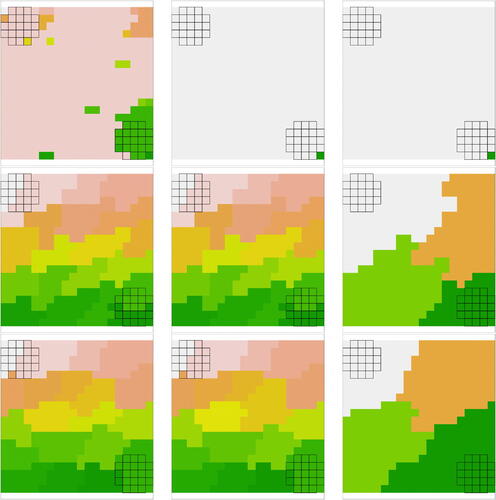
To better understand the performance differences in Table 1, for an individual simulation where the change-point for ${\text{cl}}_2$ happens at time 90, Figure 2 shows the clustering outcomes of the nine combinations of considered linkage functions and methods to estimate the optimal number of clusters. The two grids in the corners show the positions of clouds ${\text{cl}}_1$ and ${\text{cl}}_2$ in this example and different colors represent distinct estimated clusters. We can see that none of the combinations is able to precisely detect the borders of the clouds. The combinations of Complete and Ward.D2 with Dunn2 generally seem to lead to similar classification of the pixel time series. Both encapsulate the clouds in regions that are bigger than the actual clouds. On the contrary, the combinations of Complete and Ward.D2 with Ch/Dunn propose clusters that partially cover the clouds, whereby parts of the clouds belong to different estimated clusters. The joint performance of Single and Dunn/Dunn2 performs quite poorly, as it is not able to properly distinguish between the pixel time series in ${\text{cl}}_1,{\text{cl}}_2$, and the rest of the image. Finally, when the Single linkage is combined with Ch it apparently detects the border of one of the clouds. Moreover, generally, the Single linkage function seems to often introduce singular pixels as clusters.

Fig. 2 An individual example (one out of 200 simulations) of the clustering results for Scenario I, with spatially correlated pixel time series, when the change-point for ${\text{cl}}_2$ happens at time 90. Rows from top to bottom: Single, Complete, and Ward.D2 linkage functions. Columns from left to right: Ch, Dunn, and Dunn2. Each color represents a cluster, and the two clouds are displayed as two grids in the corners.

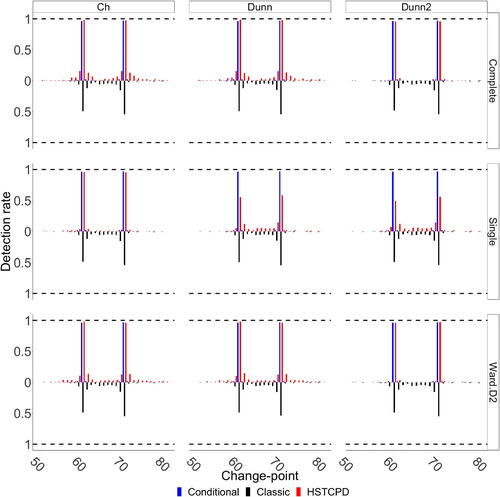
Figure 3 shows the detection rate for all detected change-points based on all considered combinations of clustering approaches, including Classic and Conditional, when the change-point for ${\text{cl}}_2$ is 70. The results concerning the cases where the change for ${\text{cl}}_2$ happens at time 90 or 120 can be found in Section S2.1.1 (see Figures S1 and S2). Overall, we can see that the Classic approach performs quite poorly; the change-point for ${\text{cl}}_1$ is precisely detected only 49% of the time and that for ${\text{cl}}_2$ is detected only 54% of the time. More importantly, in only 69 of the 200 simulations (i.e., 34.5%) the two change-points are jointly detected with no error margin. In other words, employing no pre-classification may lead to erroneous results due to the fact that an actual change-point could be dominated/hidden by either another change-point or by pixel time series with no change blurring the detection. In addition, in Figure 3 one can see that the Classic approach sometimes detects change-points at times between the times of the actual change-points in ${\text{cl}}_1$ and ${\text{cl}}_2$.

Fig. 3 Detection rate based on 200 simulations from Scenario I, with spatially correlated pixel time series, when the change-point for ${\text{cl}}_2$ occurs at time 70.

Turning to the Conditional approach, the change in ${\text{cl}}_1$ (${\text{cl}}_2$) is precisely detected 96.5% (97%) of the time; the rate of simultaneous precise detection is 93.5%. For the rest of the cases, the changes are generally detected with an error margin of one time unit, that is, 59 or 61 for the case of ${\text{cl}}_1$ and 69 or 71 for the case of ${\text{cl}}_2$. This emphasizes the need of running a classification algorithm prior to performing change-point detection, that is, applying HSTCPD.

With respect to HSTCPD, the change-point detection performance generally depends on the quality of the pre-classification. The poorest performance in this case is that of Single-Dunn2 since, based on the SI values in Table 1, it could not sufficiently separate the two clouds; the change in ${\text{cl}}_1$ (${\text{cl}}_2$) is precisely detected 49.5% (56%) of the time, which is slightly better than the results for the Classic approach. For all other combinations, the results for HSTCPD are generally as good as for the Conditional approach. For instance, for Ward.D2-Dunn (Single-Ch) the change-points for ${\text{cl}}_1$ and ${\text{cl}}_2$ are precisely detected 98% (96%) and 96.5% (95.5%) of the time, with a simultaneous detection rate of 94.5% (92%). The (slight) difference between HSTCPD and the Conditional approach comes from the fact that (i) it may happen that there are a few pixel time series in a cloud for which the general behavior happens to differ from the expected behavior within the cloud (due to random effects), that is, outliers, and pre-classification generally excludes outliers from the detected cluster/estimated cloud, and (ii) HSTCPD may generate clusters outside the actual clouds and random effects may in turn lead the change-point detection method in question to conclude that there is a change-point in such an artificial cloud, when there in fact is not, that is, we commit a Type I error; this is reflected by the small red jumps in Figure 3. Regarding (ii), note, however, that with respect to the number of actual tests we are conducting, the proportion of Type I errors committed is in line with the chosen significance level. Excluding the outliers facilitates the change-point detection process by increasing the power and reducing the estimation error. Coming back to (ii), Ward.D2-Dunn2 and Complete-Dunn2 lead to four (large) clusters while properly separating the clouds and consequently giving rise to a high power, low estimation error, and low risk for Type I error. On the contrary, Ward.D2-Ch and Complete-Ch lead to many clusters, where the actual clouds might be part of distinct clusters, whereby the number of mistakenly detected changes increases but, as previously stated, still on par with the significance level. Note that, clearly, there is a tradeoff between the sizes of the detected clusters and the number of detected change-points.

In addition, we have seen that increasing the time difference between the two change-points in ${\text{cl}}_1$ and ${\text{cl}}_2$ improves the performance of the Classic approach, however, its general performance does not reach that of HSTCPD and would be still unable to discover the marginals undergoing changes (see Figures S1 and S2).

4.4.2 Other Scenarios

Regarding the Scenarios II and III with spatially correlated pixel time series, which are presented in Sections S2.2.1 and S2.3.1, we have similarly seen that the pre-clustering component of HSTCPD significantly enhances the change-point analysis by significantly increasing the detection rate of the Classic approach. For the situation where all marginals are both spatially and temporally independent, the corresponding results for the Scenarios I, II, and III are presented in Sections S2.1.2, S2.2.2, and S2.3.2, respectively. We have seen that, for Scenarios I and II, the combination of any of the linkage functions with Dunn leads to RI and SI being nearly one in all cases, regardless of the change-point in ${\text{cl}}_2$ (see Tables S1 and S3 and Figures S3 and S11). Consequently, such a combination leads to the best performance of HSTCPD which is in general identical to that of the Conditional approach (see Figures S4–S6 and S12–S14). With respect to Scenario III, when the time difference between the two change-points in ${\text{cl}}_1$ and ${\text{cl}}_2$ is small, none of the clustering approaches is generally able to put the two clouds in distinct clusters. However, the general performance of the considered clustering approaches improves by increasing the time difference between the two change-points according to which the combinations of Single and any of Ch, Dunn, or Dunn2, Complete-Dunn, and Ward.D2-Dunn show their best performance when the change-point in ${\text{cl}}_2$ occurs at time 120. The performance of Complete-Ch and Ward.D2-Ch does not get any better by increasing the time difference between the two change-points. For Complete-Dunn2 and Ward.D2-Dunn2, their performances get only slightly better when the change-point in ${\text{cl}}_2$ occurs at time 120 (See Table S5 and Figure S19). The detection rates for all three approaches in scenario III are presented in Figures S20–S22.

Fig. 4 Detection rate based on 200 simulations from Scenario I, with spatially correlated pixel time series, when the change-point for ${\text{cl}}_2$ occurs at time 70.

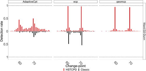
We further apply the methods of Liu et al. (2020) and Grundy, Killick, and Mihaylov (2020) to the situation where there exists spatial correlation between the pixel time series, when the change-point for ${\text{cl}}_2$ happens at times 70, 90, and 120. The corresponding results for these two methods can be found in Sections S2.4 and S2.5. We see that, in general, the pre-classification enhances the performance of the adaptive method of Liu et al. (2020). However, it performs poorer than the method of Matteson and James (2014), which is a consequence of spreading out the estimated change-points around the actual change-points leading to a lower precise detection rate. The geometrical mapping approach of Grundy, Killick, and Mihaylov (2020) performs quite poor in the absence of pre-classification, having a detection rate near zero for most cases, especially those in Scenario I. Nevertheless, its performance significantly enhances when HSTCPD is applied to it, yielding a detection rate of around 97%. For a general comparison of the three considered approaches in the absence (Classic) and presence (HSTCPD) of pre-classification, Figure 4 shows their detection rates under Scenario I, using Ward.D2-Dunn, when the change-point for ${\text{cl}}_2$ occurs at time 70. The biggest impact of pre-classification can be seen in the geometrical mapping approach (i.e., geomcp) which is somehow expected as it is based on global dimension reduction.

Turning to (i) multiple changes in the mean of each cloud, (ii) existence of both mean and variance changes in each cloud, and (iii) scalability of HSTCPD, we add that their corresponding results are presented in Sections S2.6, S2.7, and S2.8, respectively. The general take away message in these situations is that HSTCPD clearly outperforms the state-of-the-art, even on large image time series, and geomcp sometimes mistakenly detects changes in the mean as if they were changes in the variance and vice versa.

5 Real Data Analyses

This section is devoted to applying our proposal to two sets of real data: (i) Land Surface Temperature (LST) in Spain from February 2000 to November 2021, and (ii) The WikiLeaks Afghan War Diary (AWD) data (Zammit-Mangion et al. 2012), which runs monthly from January 2004 to December 2009. Note that, generally speaking, identifying change-points could indicate changes in the underlying data-generating processes, and consequently lead to improved modeling by incorporating this information. Throughout we employ the Ward.D2 linkage and the Dunn approach to estimate the optimal clusters. We let the maximum number of clusters be 150 when searching for optimal clusters. Since our image time series may exhibit seasonality, we make use of their deseasoned versions, that is, the monthly anomalies, to look for change-points based on the method of Matteson and James (2014).

5.1 Land Surface Temperature (LST) in Spain from 2000 to 2021

As an effect of climate change, in recent years, southern European countries have experienced extreme weather conditions, with, for example, rapid temperature changes, and it has been hypothesized that weather conditions are becoming more extreme (Toreti et al. 2019). Such changes may, however, vary regionally, and we here wish to understand how Spain has been subjected to this phenomenon in the last two decades. More specifically, we here study the image time series of LST in continental Spain, which is a region of 505,944 ${\text{km}}^2$. Since the study region is large, we use the Modis Terra satellite which leads to 17GB of images that are downloaded from the MOD11C3 product (Wan, Hook, and Hulley 2015). For the selected period, February 2000 to November 2021, we deal with one image per month and that leads to a total of 262 images, represented in Figure S47. Each image captures the monthly average LST derived from the daily collected data, which have been put together and cropped to obtain a monthly image with a resolution of $253\times 147=39,721$ pixels per image; this means handling this amount of marginals when performing change-point analysis. All downloading and processing are carried out using the $\mathsf{R}$ package $\mathsf{rsat}$ (Pérez-Goya et al. 2022). See Section S3.1 for more details about the data.

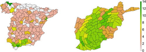
The left panel of Figure 5 shows the optimal clusters for the LST data together with their corresponding numbers of detected change-points. There are various clusters with no change-point which are generally located in the north. The majority of the rest of the clusters face change-points, but at dissimilar times. Figure S48 shows the estimated change-points per clusters, revealing the changes which could not be detected if one does not follow a pre-classification approach; in this case, one can only detect two change-points at times 199 and 217, which correspond to the months August, 2016, and February, 2018. Note in particular that these change-points occur toward the end of the study period. Furthermore, according to HSTCPD the majority of the estimated clusters also undergo changes at such times which means that these changes dominate other change-points and/or regions with no change-points if one does not carry out clustering prior to the change-point analysis. In addition, one can see that the distribution of both numbers and times of the detected change-points is spatially dependent.

Fig. 5 Change-point detection, based on HSTCPD, for LST data in Spain (left), and AWD data of Afghanistan (right). Each sub-region, obtained via Ward.D2-Dunn, represents a single cluster and numerical values are the number of detected change-points.

5.2 Afghan War Data

The original data consists of roughly 77,000 events, representing anything from a stop-and-search episode to a gun fight in which the U.S. military was involved, which reduces to 75,239 events after excluding the points which are placed outside the boundary of Afghanistan. Figure S50 shows the AWD data from which one can see that most events occurred in the east and south-east of Afghanistan. We are here interested in looking for change-points in the time-ordered intensity surfaces corresponding to such spatial point patterns, and check if the behavior of possible change-points is spatially dependent. In particular, such an analysis allows us to elucidate where and when the underlying conflict may have escalated. Hence, for each point pattern in Figure S50, an intensity surface is estimated using a kernel-based estimator with the Jones-Diggle edge correction (Baddeley, Rubak, and Turner 2015, chap. 6) and a common bandwidth which is obtained as the geometrical mean of individual bandwidths for each pattern based on the criterion of Cronie and Van Lieshout (2018). See the estimated intensities in Figure S51; each image is based on 7756 pixels, within the boundary of Afghanistan, which means dealing with this amount of marginals when performing multivariate change-point detection. See Section S3.2 for a further description of the data and the estimated intensity surfaces.

The right panel of Figure 5 shows the 99 optimally estimated clusters for the image time series of the estimated intensities, together with the corresponding numbers of change-points. One can see that the number of estimated change-points varies spatially across Afghanistan, showing that the estimated intensities, and thereby the conflicts, in the north-east, north-west and south-east are more stable as for having less change-points compared to the rest of Afghanistan. Moreover, we see that there are sub-regions behaving differently compared to their neighbors, thus, emphasizing the non-separable nature of the data. In Figure S52 we present the estimated change-points per cluster, disclosing the change-points that could not be detected if one ignores the pre-clustering/classification which consequently results in detecting only five change-points without gaining any knowledge of where they occur.

6 Discussion

A key step in HSTCPD is the way one performs clustering which clearly influences its general performance. Here, we have considered hierarchical clustering for spatially dependent functions; however, one may employ other clustering approaches (e.g., non-Euclidean distance-based approaches), linkage functions, and/or methods to discover the optimal number of clusters. Overall, we recommend trying various methods and, then, taking data characteristics and possible prior knowledge/assumptions into account, choosing the results which tend to better suit such characteristics and assumptions. Moreover, we recommend avoiding clustering approaches which, proportional to the dimension of data, give rise to too large or too small clusters. The former may not properly separate sub-regions with different behaviors, while the latter may split similar data into smaller clusters. Too large clusters may lead to results which still suffer from masking/domination, and too small clusters may diminish the general performance of multivariate change-point methods. Moreover, multivariate change-point detection methods different from those of Matteson and James (2014), Liu et al. (2020), and Grundy, Killick, and Mihaylov (2020) may be considered. Future work includes exploring such variations. Finally, we emphasize that the idea behind HSTCPD can be applied to nonspatial settings as masking/concealment among different marginals/components can happen in general multivariate settings. In this line of reasoning, we believe that our method is widely generally applicable in many applied contexts and real data settings, and as such can be helpful to various applied researchers with a need to detect change-points.

Supplementary Materials

The supplementary material contains additional background to the manuscript, including some preliminaries on multivariate change-point detection, and hierarchical clustering with details regarding linkage functions, and methods to estimate optimal clusters for spatially dependent data in Section S1. Additional simulation studies can be found in Section S2 which cover various scenarios concerning changes in the mean, the variance, multiple changes, and scalability of HSTCPD. Further descriptions and results about our real datasets (i.e. LST in Spain from February 2000 to November 2021, and AWD data which runs monthly from January 2004 to December 2009) are also presented in Section S3.

Acknowledgments

The authors are grateful to the editor and two reviewers for useful comments. The authors are also grateful to Yufeng Liu for supplying the R code of the AdaptiveCpt method. All the presented results are reproducible, and the corresponding R code can be found at https://github.com/Moradii/HSTCPD.

Disclosure Statement

The authors report there are no competing interests to declare.

References

- Aminikhanghahi, S., and Cook, D. J. (2017), “A Survey of Methods for Time Series Change Point Detection,” Knowledge and Information Systems, 51, 339–367. DOI: 10.1007/s10115-016-0987-z.
- Aston, J. A., and Kirch, C. (2012), “Detecting and Estimating Changes in Dependent Functional Data,” Journal of Multivariate Analysis, 109, 204–220. DOI: 10.1016/j.jmva.2012.03.006.
- Baddeley, A., Rubak, E., and Turner, R. (2015), Spatial Point Patterns: Methodology and Applications with R, Boca Raton, FL: CRC Press.
- Berkes, I., Gabrys, R., Horváth, L., and Kokoszka, P. (2009), “Detecting Changes in the Mean of Functional Observations,” Journal of the Royal Statistical Society, Series B, 71, 927–946. DOI: 10.1111/j.1467-9868.2009.00713.x.
- Cressie, N., and Wikle, C. K. (2015), Statistics for Spatio-Temporal Data, Hoboken, NJ: Wiley.
- Cronie, O., and Van Lieshout, M. N. M. (2018), “A Non-Model-based Approach to Bandwidth Selection for Kernel Estimators of Spatial Intensity Functions,” Biometrika, 105, 455–462. DOI: 10.1093/biomet/asy001.
- Grundy, T. (2020), changepoint.geo: Geometrically Inspired Multivariate Changepoint Detection. R package version 1.0.1.
- Grundy, T., Killick, R., and Mihaylov, G. (2020), “High-Dimensional Changepoint Detection via a Geometrically Inspired Mapping,” Statistics and Computing, 30, 1155–1166. DOI: 10.1007/s11222-020-09940-y.
- Hahn, G., Fearnhead, P., and Eckley, I. A. (2020), “Bayesproject: Fast Computation of a Projection Direction for Multivariate Changepoint Detection,” Statistics and Computing, 30, 1691–1705. DOI: 10.1007/s11222-020-09966-2.
- Horváth, L., and Rice, G. (2014), “Extensions of Some Classical Methods in Change Point Analysis,” Test, 23, 219–255. DOI: 10.1007/s11749-014-0368-4.
- James, N. A., and Matteson, D. S. (2015), “ecp: An R package for Nonparametric Multiple Change Point Analysis of Multivariate Data,” Journal of Statistical Software, 62, 1–25.
- Liu, B., Zhou, C., Zhang, X., and Liu, Y. (2020), “A Unified Data-Adaptive Framework for High Dimensional Change Point Detection,” Journal of the Royal Statistical Society, Series B, 82, 933–963. DOI: 10.1111/rssb.12375.
- Matteson, D. S., and James, N. A. (2014), “A Nonparametric Approach for Multiple Change Point Analysis of Multivariate Data,” Journal of the American Statistical Association, 109, 334–345. DOI: 10.1080/01621459.2013.849605.
- Moradi, M., Montesino-SanMartin, M., Ugarte, M. D., and Militino, A. F. (2022), “Locally Adaptive Change-Point Detection (LACPD) with Applications to Environmental Changes,” Stochastic Environmental Research and Risk Assessment, 36, 251–269. DOI: 10.1007/s00477-021-02083-0.
- Page, E. (1954), “Continuous Inspection Schemes,” Biometrika, 41, 100–115.
- Page, E. (1955), “A Test for a Change in a Parameter Occurring at an Unknown Point,” Biometrika, 42, 523–527.
- Pérez-Goya, U., Montesino-SanMartin, M., Militino, A. F., and Ugarte, M. D. (2022), rsat: Dealing with Multiplatform Satellite Images from Landsat, MODIS, and Sentinel. R package version 0.1.19.
- Ramsey, J., and Silverman, B. W. (2005), Functional Data Analysis, New York: Springer.
- Rand, W. (1971), “Objective Criteria for the Evaluation of Clustering Methods,” Journal of the American Statistical Association, 66, 846–850. DOI: 10.1080/01621459.1971.10482356.
- Sundararajan, R. R., and Pourahmadi, M. (2018), “Nonparametric Change Point Detection in Multivariate Piecewise Stationary Time Series,” Journal of Nonparametric Statistics, 30, 926–956. DOI: 10.1080/10485252.2018.1504943.
- Toreti, A., Belward, A., Perez-Dominguez, I., Naumann, G. et al. (2019), “The Exceptional 2018 European Water Seesaw Calls for Action on Adaptation,” Earth’s Future, 7, 652–663. DOI: 10.1029/2019EF001170.
- Truong, C., Oudre, L., and Vayatis, N. (2020), “Selective Review of Offline Change Point Detection Methods,” Signal Processing, 167, 107299. DOI: 10.1016/j.sigpro.2019.107299.
- Wan, Z., Hook, S., and Hulley, G. (2015), “Mod11c3 modis/terra Land Surface Temperature/Emissivity Monthly l3 Global 0.05 deg cmg v006,” NASA EOSDIS LP DAAC.
- Wang, T., and Samworth, R. J. (2018), “High Dimensional Change Point Estimation via Sparse Projection,” Journal of the Royal Statistical Society, Series B, 80, 57–83. DOI: 10.1111/rssb.12243.
- Xiong, L., Jiang, C., Xu, C., Yu, K.-x., Guo, S. (2015), “A Framework of Change-Point Detection for Multivariate Hydrological Series,” Water Resources Research, 51, 8198–8217. DOI: 10.1002/2015WR017677.
- Zammit-Mangion, A., Dewar, M., Kadirkamanathan, V., and Sanguinetti, G. (2012), “Point Process Modelling of the Afghan War Diary,” Proceedings of the National Academy of Sciences, 109, 12414–12419. DOI: 10.1073/pnas.1203177109.
- Zhang, N. R., Siegmund, D. O., Ji, H., and Li, J. Z. (2010), “Detecting Simultaneous Changepoints in Multiple Sequences,” Biometrika, 97, 631–645. DOI: 10.1093/biomet/asq025.