Using Conformal Win Probability to Predict the Winners of the Canceled 2020 NCAA Basketball Tournaments

Abstract

The COVID-19 pandemic was responsible for the cancellation of both the men’s and women’s 2020 National Collegiate Athletic Association (NCAA) Division I basketball tournaments. Starting from the point when the Division I tournaments and unfinished conference tournaments were canceled, we deliver closed-form probabilities for each team of making the Division I tournaments, had they not been canceled, under a simplified method for tournament selection. We also determine probabilities of a team winning March Madness, given a tournament bracket. Our calculations make use of conformal win probabilities derived from conformal predictive distributions. We compare these conformal win probabilities to those generated through linear and logistic regression on college basketball data spanning the 2011–2012 and 2022–2023 seasons, as well as to other publicly available win probability methods. Conformal win probabilities are shown to be well calibrated, while requiring fewer distributional assumptions than most alternative methods.

Keywords:

• Conformal inference
• Elo
• Kaggle
• March Madness
• Predictive distributions
• Ranking
• Sports analytics
• Uncertainty quantification

1 Introduction

Two of the most popular tournaments in the world are the men’s and women’s National Collegiate Athletic Association (NCAA) Division I basketball tournaments, colloquially known as March Madness. In college basketball, teams are grouped into conferences. During the regular season, teams compete against opponents within their own conference as well as teams outside their conference. Following the regular season, better performing teams within each conference compete in a conference tournament, with the winner earning an invitation to play in the Division I (DI) tournament. The invitation for winning a conference tournament is called an “automatic bid.” Historically, 64 teams are selected for the women’s tournament. Thirty-two of the 64 teams are automatic bids, corresponding to the 32 conference tournament winners. The other 32 teams are “at-large bids,” made up of teams failing to win their respective conference tournament. At-large bids are decided by a selection committee, which uses both subjective guidelines and strict constraints to choose the teams invited to the tournament and how to set the tournament bracket, which defines who and where each team will play initially and could play eventually. Teams that earn an automatic bid or an at-large bid are said to have “made the tournament.”

As a result of the COVID-19 pandemic, the NCAA canceled both the men’s and women’s 2020 NCAA tournaments. A majority of college athletic conferences followed by canceling their own conference tournaments, leaving many automatic bids for March Madness undecided. These cancellations raise natural questions about which teams might have made the March Madness field and which teams might have won the tournament. Using data from the 2019 to 2020 men’s and women’s collegiate seasons, we deliver probabilistic answers to these questions.

Specific to the 2019–2020 NCAA DI season(s), we contribute the following: (a) an overall ranking of the top Division I teams, as well as estimates of each team’s strength, based on 2019–2020 regular season data, (b) closed-form calculations for probabilities of teams making the 2019–2020 March Madness field under a simplified tournament selection process, calculated from the point when each conference tournament was canceled, and (c) closed-form calculations of probabilities of teams winning March Madness, given each of several potential brackets.

The calculation of probabilities for teams making the 2019–2020 March Madness field considers each conference tournament’s unfinished bracket as well as our estimates of DI team strengths, which we fix following the culmination of the regular season. The closed-form nature of the probabilities also reduces the computational load and eliminates error inherent to simulation-based approaches. To our knowledge, this is the first closed-form approach to take into account partially completed conference tournaments when generating probabilities of making the March Madness field.

Estimating March Madness win probabilities prior to the selection of the tournament field and the determination of the March Madness bracket is a difficult problem. If we define all the potential brackets as the set $\mathcal{B}$ and $\{W_u=1\}$ as the event where team u wins March Madness, we can decompose $\mathbb{P}(W_u=1)$ as (1) $$\mathbb{P}(W_u=1)=\sum _{B\in \mathcal{B}}\mathbb{P}(W_u=1|B)\mathbb{P}(B).$$(1)

However, calculations for all possible brackets within $\mathcal{B}$ are intractable. For a set of, say, 350 teams, there are $(\begin{array}{c}350\\ 64\end{array})$ ways to select a field of teams to compete in a 64-team tournament. Given a tournament field of $N=2^J$ teams, where J is the number of rounds in the tournament (J = 6 for a 64-team tournament), the number of unique brackets for a single-elimination tournament is (2) $$\prod _{i=1}^{N/2}\left(\begin{array}{c}2i\\ 2\end{array}\right)/2^{N/2-1},$$(2) which grows rapidly as N increases. An 8-team tournament results in 315 potential brackets, while a 16-team tournament results in 638,512,875 potential brackets. In the case of March Madness, the size of the set $\mathcal{B}$ is enormous.

Of course, some brackets are more likely than others due to the set of constraints used by the selection committee. Even if the set of plausible brackets for March Madness was small relative to the complete set $\mathcal{B}$ when the tournaments were canceled in 2020, estimating $\mathbb{P}(B)$ in (1) for any given bracket B depends on the complex and, ultimately, subjective decision making process used by the NCAA selection committee.

While we can explicitly construct $\mathbb{P}(B)$ under the simplified tournament selection process outlined in this article, the calculation is often computationally difficult. Thus, we make no attempt to calculate $\mathbb{P}(B)$ for any bracket B. Instead, in this article, we focus on the construction of the marginal probability of each team making the March Madness field. Additionally, using brackets suggested by experts, along with brackets we construct, we compare March Madness win probabilities, $\mathbb{P}(W_u=1|B)$ for all teams u, across different brackets B. We find that the win probabilities for teams most likely to win are relatively stable across brackets. Baylor, South Carolina, and Oregon each had more than a 20% win probability for most of the brackets we considered for the women’s tournament. On the men’s side, Kansas was the most likely to win the tournament regardless of the bracket.

Another contribution of the article is the novel application of conformal predictive distributions (Vovk et al. 2019) for the estimation of win probability, aptly named conformal win probability. Conformal predictive distributions allow for the construction of win probability estimates under very mild distributional assumptions, reducing dependence on, say, normality assumptions, for our results. When compared using both men’s and women’s post-season NCAA basketball spanning the 2011–2012 and 2022–2023 seasons, we find that conformal predictive distributions provided win probability estimates that often performed better than other methods, including well-performing, publicly available models.

Section 2 provides background on constructing overall win probabilities for single-elimination tournaments and introduces the closed-form calculation of probabilities related to March Madness. Section 3 describes three methods for generating win probabilities of individual games, including the construction of conformal win probability estimates. Section 4 describes the overall results, including a ranking of the top teams, conference tournament and March Madness win probabilities associated with the 2019–2020 NCAA DI basketball season and a comparison of win probability generation methods. Section 5 concludes the article. All of the R code and datasets used in this research are available at https://github.com/chancejohnstone/marchmadnessconformal.

2 Probabilities for March Madness

In this section, we describe win probability as it relates to single-elimination tournaments like March Madness. We also introduce the probability of a team making the March Madness field, given a collection of conference tournament brackets, team strengths and game-by-game win probabilities. We limit our discussion scope in this section primarily to the women’s tournament, but the general construction reflects the men’s tournament also.

Throughout this article, we use the common verbiage that a team is ranked “higher” than another team if the former team is believed to be better than the latter team. Likewise, a “lower” ranking implies a weaker team. We follow the common convention that a team of rank r has a higher rank than a team of rank s when r < s. Teams ranked 1 to 32 are collectively identified as “high-ranked.” Teams ranked below 64 are identified as “low-ranked.” While the colloquial use of the term “bubble teams” is usually reserved to describe a subset of teams near the boundary separating teams in and out of the March Madness field, we use the term to explicitly describe the teams ranked 33 to 64. In Section 3.3, we discuss an approach to rank teams based on observed game outcomes.

2.1 Win Probability for Single-Elimination Tournaments

Given a collection of game-by-game win probabilities, one method for providing estimates of overall tournament win probability is through simulation. Suppose that for a game between any pair of teams u and v in our tournament, we have the probability that team u defeats team v, defined as p_uv . While the true value of p_uv is not known in practice, we describe methods for estimating the probability for any match-up in Section 3. We can simulate the outcome of a game between team u and team v by randomly sampling from a standard uniform distribution. A value less than p_uv corresponds to a victory for team u, while a value greater than p_uv represents a victory for team v. Every game in a tournament can be simulated until we have an overall winner. We can then repeat the entire simulation process multiple times to get a Monte Carlo estimate of each team’s probability of winning said tournament.

Suppose we have an eight team single-elimination tournament with the bracket shown in Figure 1. The highest ranking team, team 1, plays the lowest ranking team, team 8, in the first round. Assuming team 1 was victorious in round one, their second round opponent could be team 4 or 5. In the third round, team 1 could play team 3, 6, 2, or 7. After the first round of the tournament, team 8 has the same potential opponents as team 1.

Fig. 1 Bracket for eight-team single-elimination tournament.

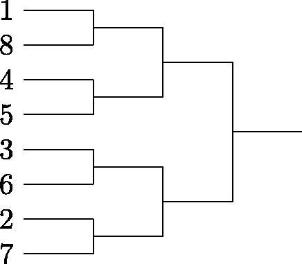
Using the knowledge of a team’s potential opponents in future games, we can calculate win probabilities for any upcoming round and, thus, the entire tournament. Formalized in Edwards (1991), the tournament win probability for team u given a fixed, single-elimination tournament bracket with J rounds is (3) $$q_{uJ}=q_{uJ-1}\left[\sum _{s\in {\mathcal{O}}_{uJ}}{p}_{us}{q}_{sJ-1}\right],$$(3) where q_uj is the probability that team u wins in round $j=1,\dots ,J$, and ${\mathcal{O}}_{uj}$ is the set of potential opponents team u could play in round j. We explicitly set $q_{u1}=p_{u{\mathcal{O}}_{u1}}$, where ${\mathcal{O}}_{u1}$ is team u’s opponent in round one. We can extend (3) to single-elimination tournaments of any size or construction as long as we are able to determine the set ${\mathcal{O}}_{uj}$ for any team u in any round j.

2.2 Probability for Making the NCAA Tournament

With (3) we can generate an overall tournament win probability for each team in a tournament exactly, given a fixed tournament bracket and game-by-game win probabilities. However, following the regular season, but prior to the culmination of all conference tournaments, the field for March Madness is not fully known. Thus, we cannot use (3) directly for estimating team win probabilities for the 2020 March Madness tournament. We first turn our attention to estimating each women’s team’s probability of making the 2020 March Madness field, made up of 32 automatic bids and 32 at-large bids. Although the closed-form calculations reflect probabilities related to the 2019–2020 women’s March Madness tournament, which would have included 64 teams, only slight changes are required to reflect the inclusion of 68 teams, that is, to account for the “First Four” play-in games in both the men’s and women’s tournaments. We include a description of the First Four play-in system in supplementary materials. A 68 team tournament is used for results pertaining to the 2019–2020 men’s March Madness tournament contained in supplementary materials.

We define F_u as the indicator variable for whether or not the u-th ranked team makes the NCAA tournament field. Knowing that the NCAA tournament is made up of automatic and at-large bids, we define two relevant indicator variables C_u and L_u associated with a team receiving one of these bids, respectively. C_u is one if team u wins its conference tournament and zero otherwise. We define L_u as the number of conference tournaments won by teams ranked below team u. Then, under the assumption that higher-ranked at-large bids make the March Madness field before lower-ranked at-large bids, for any team u, the probability of making the NCAA tournament is (4) $$\begin{array}{c}\mathbb{P}(F_u=1)=\mathbb{P}(\{C_u=1\}\cup \{L_u\le t_u\})\\ =\mathbb{P}(C_u=1)+\mathbb{P}(L_u\le t_u)-\mathbb{P}(C_u=1,L_u\le t_u),\end{array}$$(4) where $t_u=64-u$ is the maximum number of teams ranked below team u that can receive an automatic bid without preventing team u from receiving an at-large bid. Because there are 32 conference tournaments, $\mathbb{P}(L_u\le 32)=1$. Thus, with the current construction, teams ranked 32 $(64-32)$ or higher always make the NCAA tournament. For low-ranked teams, (4) reduces to $\mathbb{P}(C_u=1)$; weaker teams must win their conference tournament to get an invite to March Madness.

We can decompose the intersection probability of (4) into (5) $$\mathbb{P}(C_u=1,L_u\le t_u)=\mathbb{P}(L_u\le t_u|C_u=1)\mathbb{P}(C_u=1).$$(5)

To explicitly describe the probabilities in (5), we split the teams in each conference into two sets, ${\mathcal{H}}_k^u$ and ${\mathcal{L}}_k^u$, defining ${\mathcal{H}}_k^u$ as the set of teams in conference $k=1,\dots ,K$ ranked higher than or equal to team u and ${\mathcal{L}}_k^u$ as the set of teams in conference k ranked lower than team u. We reference lower or higher-ranked teams in the same conference as team u using k(u) instead of k. Note that team $u\in {\mathcal{H}}_{k(u)}^u$. Let $C_{{\mathcal{H}}_k^u}=1$ if a team in ${\mathcal{H}}_k^u$ wins conference tournament k and 0 otherwise. $C_{{\mathcal{L}}_k^u}$ is defined in a similar manner for teams in ${\mathcal{L}}_k^u$.

We assume that the outcome of any conference tournament is independent of the outcome of any other conference tournament. Thus, we can describe L_u as a sum of independent, but not identically distributed, Bernoulli random variables, (6) $$L_u=\sum _{k=1}^K{C}_{{\mathcal{L}}_k^u}.$$(6)

If $C_{{\mathcal{L}}_k^u}$ were identically distributed for all conferences, then L_u would be a binomial random variable. Because this is not the case, L_u is instead a Poisson-binomial random variable with cumulative distribution function (7) $$\mathbb{P}(L_u\le l)=\sum _{m=0}^l\left\{\sum _{A\in {\mathcal{F}}_m}\prod _{s\in A}{p}_s\prod _{s\in A^C}(1-p_s)\right\},$$(7) where p_k is the probability of a team in ${\mathcal{L}}_k^u$ winning conference tournament k, and ${\mathcal{F}}_m$ is the set of all unique m-tuples of $\{1,\dots ,32\}$. With (7) known, the conditional portion of (5) is a new Poisson-binomial random variable where $p_{k(u)}=0$; we condition on team u winning their conference tournament. Thus, the probability of team u making the tournament is (8) $$\begin{array}{c}\mathbb{P}(F_u=1)=q_{u{J}_{k(u)}}+\mathbb{P}(L_u\le t_u)\\ \hspace{1em}-(\sum _{m=0}^{t_u}\{\sum _{A\in {\mathcal{F}}_m}\prod _{s\in A}p{\prime }_s\prod _{s\in A^C}(1-p{\prime }_s)\})\times q_{u{J}_{k(u)}},\end{array}$$(8) where $p{\prime }_k$ is equal to p_k when k is not equal to k(u) and zero otherwise, and $J_{k(u)}$ is the number of rounds in the conference tournament for conference k(u).

While the above derivation provides a closed-form calculation for probabilities of making the March Madness field, it does not describe any team’s probability of winning March Madness. To do this, we must also derive closed-form probability calculations for specific tournament brackets. However, as discussed in Section 1, it is difficult to explicitly construct calculations for this task due to the inherent subjectivity associated with the seeding of teams. For this reason, we focus on the probability of each team making the March Madness field and, given a March Madness bracket, the probability of each team winning the March Madness tournament. Additionally, we emphasize that while a primary focus of this article is to explore the canceled 2020 tournaments, the results laid out in this section can be applied to any post-season in progress, allowing for March Madness field probability updates as teams are eliminated from their respective conference tournaments.

3 Win Probabilities for Individual Games

Determining win probability in sports primarily began with baseball (Lindsey 1961). Since then, win probability has permeated many sports and become a staple for discussion among sports analysts and enthusiasts. Applications of win probability have been seen in sports such as basketball (Loeffelholz, Bednar, and Bauer 2009), hockey (Gramacy, Jensen, and Taddy 2013), soccer (Robberechts, Van Haaren, and Davis 2019), football (Stern 1991; Lock and Nettleton 2014), darts (Liebscher and Kirschstein 2017), rugby (Lee 1999), cricket (Asif and McHale 2016), table tennis (Liu, Zhuang, and Wan 2016) and even video games (Semenov et al. 2016), among others.

These methods typically use some form of parametric regression to capture individual and/or team strengths, offensive and/or defensive capabilities or other related effects. We continue the parametric focus by using a linear model to estimate team strengths, but our approach makes minimal distributional assumptions.

Initially, suppose that (9) $$y_i=x_i^{\prime }\beta +{ϵ}_i,$$(9) where y_i represents the response of interest for observation i, x_i is a length p vector of covariates for observation i, β is the vector of parameter values and ϵ_i is a mean-zero error term. We define $y=(y_1,\dots ,y_n)\prime$ and $X=(x_1,\dots ,x_n)\prime$, where the vector y and matrix X make up our n observations $D_n={\{(x_i,y_i)\}}_{i=1}^n$. In subsequent sections, the response values in y will be margin of victory (MOV), and the elements of β will include team strength parameters. However, at this stage a slightly more general treatment is useful.

We next discuss event probability estimation via three different methods: conformal predictive distributions based on model (9), linear regression with model (9) and an added assumption of mean-zero, independent and identically distributed normal errors, and logistic regression.

3.1 Event Probability with Conformal Predictive Distributions

Predictive distributions (Lawless and Fredette 2005) provide a method for estimating the conditional distribution of a future observation given observed data. Conformal predictive distributions (CPDs) (Vovk et al. 2019) provide similar results using a distribution-free approach based on conformal inference (Gammerman, Vovk, and Vapnik 1998). The next section contains a general treatment of conformal inference, followed by an introduction to conformal predictive distributions.

3.1.1 Conformal Inference

In a regression context, conformal inference (Gammerman, Vovk, and Vapnik 1998; Vovk, Gammerman, and Shafer 2005) produces conservative prediction regions for some unobserved response $y_{n+1}$ through the repeated inversion of some hypothesis test, say (10) $$H_0:y_{n+1}=y_c\text{ versus }{H}_a:y_{n+1}\ne y_c,$$(10) where $y_{n+1}$ is the response value associated with an incoming covariate vector $x_{n+1}$, and y_c is a candidate response value (Lei et al. 2018). The only assumption required to achieve valid prediction intervals is that the data D_n combined with the new observation $(x_{n+1},y_{n+1})$ comprise an exchangeable set of observations.

The inversion of (10) is achieved through refitting the model of interest with an augmented dataset that includes the data pair $(x_{n+1},y_c)$. For each candidate value, a set of conformity scores is generated, one for each observation in the augmented dataset, which measure how well a particular data point conforms to the rest of the dataset; traditionally a conformity score is the output of a function of the data pair (x_i , y_i ) and the prediction for y_i , denoted ${\widehat{y}}_i(y_c)$, as arguments. While the prediction ${\widehat{y}}_i(y_c)$ is dependent on both $(x_{n+1},y_c)$ and D_n , we omit dependence on $x_{n+1}$ and D_n in our notation. We define (11) $$\begin{array}{c}\pi (y_c,\tau )=\frac{1}{n+1}\sum _{i=1}^{n+1}\left[\mathbb{I}\right\{R_i(y_c)<R_{n+1}(y_c)\}+\tau \mathbb{I}\{R_i(y_c)\\ =R_{n+1}(y_c)\left\}\right],\end{array}$$(11) where, for $i=1,\dots ,n,R_i(y_c)$ is the conformity score for the data pair (x_i , y_i ) as a function of $(x_{n+1},y_c),R_{n+1}(y_c)$ is the conformity score associated with $(x_{n+1},y_c)$, and τ is a U(0, 1) random variable.

In hypothesis testing we define a p-value as the probability of a value as or more extreme than the observed test statistic under the assumption of a specified null hypothesis. With the construction of $\pi (y_c,\tau )$, we generate an estimate of the probability of an observation less extreme (or of equal extremeness) than the candidate value y_c . Thus, $1-\pi (y_c,\tau )$ provides a p-value associated with (10) (Lei et al. 2018). The inclusion of the random variable τ generates a smoothed conformal predictor (Vovk, Gammerman, and Shafer 2005).

For a fixed τ, we can construct a conformal prediction region for the response associated with $x_{n+1}$, (12) $$C_{1-\alpha ,\tau }(x_{n+1})=\{y_c\in \mathbb{R}:(n+1)\pi (y_c,\tau )\le \lceil (1-\alpha )(n+1)\rceil \},$$(12) where $1-\alpha$ is the nominal coverage level. When τ is one, $\pi (y_c,1)$ is the proportion of observations in the augmented dataset whose conformity score is less than or equal to the conformity score associated with candidate value y_c . Regardless of the conformity score or the model used to generate point predictions, a conformal prediction region with nominal coverage level $1-\alpha$ is conservative. Thus, for some new observation $(x_{n+1},y_{n+1})$, (13) $$\mathbb{P}(y_{n+1}\in C_{1-\alpha ,\tau }(x_{n+1}))\ge 1-\alpha .$$(13)

3.1.2 Conformal Predictive Distributions

One commonly used conformity score in a regression setting is the absolute residual, $|y_i-{\widehat{y}}_i(y_c)|$, which leads to symmetric prediction intervals for $y_{n+1}$ around a value $\tilde{y}$ satisfying $\tilde{y}={\widehat{y}}_{n+1}(\tilde{y})$. The traditional residual associated with a prediction, $y_i-{\widehat{y}}_i(y_c)$, results in a one-sided prediction interval for $y_{n+1}$ of the form $(-\infty ,u(D_n,x_{n+1}))$. Additionally, the selection of the traditional residual as our conformity score turns $\pi (y_c,\tau )$ into a conformal predictive distribution (Vovk et al. 2019), which provides more information with respect to the behavior of random variables than, say, prediction intervals. For example, with a CPD, we can provide an estimate of the probability of the event $y_{n+1}\le y^{*}$. For the remainder of this article we construct $\pi (·,\tau )$ using the conformity score $R_i(y_c)=y_i-{\widehat{y}}_i(y_c)$.

As previously stated, $1-\pi (y_c,\tau )$ provides a p-value associated with (10). Thus, $1-\pi (y_c,1/2)$ is analogous to the mid p-value, which acts a continuity correction for tests involving discrete test statistics. We point the interested reader to Lancaster (1961) and Barnard (1989) for additional details on the mid p-value. We set $\tau =1/2$ for the computation of our conformal predictive distributions throughout the remainder of this article.

While we have generalized conformal predictive probabilities for the event $y_{n+1}\le y^{*}$, we focus on the case where $y^{*}$ is equal to zero in later sections and instead describe probabilities associated with the event $y_{n+1}>0$, which represent win probabilities when $y_{n+1}$ is a margin of victory.

Additionally, our article focuses on models of the form shown in (9); it is important to note that conformal predictive distributions can be obtained with any other model and within other applications. In fact, they can be paired with any regression approach to generate estimates of uncertainty. Specific to the win probability application, conformal win probabilities can be used with any model where MOV is the response of interest to provide win probability estimates.

3.2 Other Event Probability Methods

We specifically outline two competing methods to conformal predictive distributions: event probability through linear regression with normal errors and event probability through logistic regression. Other popular methods for generating win probabilities include Poisson modeling (Maher 1982), Bayesian methods (Santos-Fernandez, Wu, and Mengersen 2019), rank-based (Trono 2010) and spread-based approaches (Carlin 2005), quantile regression (Bassett 2007), and nonparametric methods (Soto Valero 2016; Elfrink 2018), among others. For a comprehensive review and comparison of both win probability and outcome predictions methods, we point the interested reader to Horvat and Job (2020) and Bunker and Susnjak (2022).

3.2.1 Event Probability Through Linear Regression

We can estimate the expected value of some new observation $y_{n+1}$ using (9), but additional assumptions are required to provide event probabilities. In linear regression, the error term ϵ_i is traditionally assumed to be a mean-zero, normally distributed random variable with variance ${\sigma }^2<\infty$. Together, these assumptions with independence among error terms make up a Gauss-Markov model with normal errors (GMMNE).

A least-squares estimate for the expectation of $y_{n+1},{\widehat{y}}_{n+1}$, is $x{\prime }_{n+1}\widehat{\beta }$ where $\widehat{\beta }={(X\prime X)}^{-1}X\prime y$ when X is a full rank n × p matrix of covariates. Given the assumption of a GMMNE, ${\widehat{y}}_{n+1}$ is normally distributed with mean $x{\prime }_{n+1}\beta$ and variance ${\sigma }^2(x{\prime }_{n+1}{(X\prime X)}^{-1}{x}_{n+1})$. The prediction error for observation n + 1, $r_{n+1}=y_{n+1}-{\widehat{y}}_{n+1}$, is also normally distributed with mean zero and variance ${\sigma }^2(1+x{\prime }_{n+1}{(X\prime X)}^{-1}{x}_{n+1})$. Dividing $r_{n+1}$ by its estimated standard error then yields a t-distributed random variable. Thus, we can describe probabilities for events of the form $y_{n+1}>s$ using the standard predictive distribution (14) $$\mathbb{P}(y_{n+1}>s)=1-F_{t,n-p}\left(\frac{s-{\widehat{y}}_{n+1}}{\widehat{\sigma }\sqrt{1+x{\prime }_{n+1}{(X\prime X)}^{-}{x}_{n+1}}}\right),$$(14) where ${\widehat{\sigma }}^2=y\prime (I-X\prime {(X\prime X)}^{-1}X\prime y/(n-p)$ is the usual unbiased estimator of the error variance ${\sigma }^2$, and $F_{t,n-p}$ is the cumulative distribution function for a t-distributed random variable with n–p degrees of freedom (Wang, Hannig, and Iyer 2012).

3.2.2 Event Probability Through Logistic Regression

While linear regression allows for an estimate of $\mathbb{P}(y_{n+1}>0)$ based on assumptions related to the random error distribution, we can also generate probability estimates explicitly through logistic regression. Suppose we still have observations D_n . We define a new random variable z_i such that $z_i=\mathbb{I}\{y_i>0\}$. Instead of assumptions related to the distribution of the random error term ϵ_i , we assume a relationship between the expectation of z_i , defined as p_i , and the covariates x_i such that $\hspace{0.17em}\log \hspace{0.17em}\left(\frac{p_i}{1-p_i}\right)=x_i^{\prime }\beta$. Then, we can then derive an estimate for p_i as ${\widehat{p}}_i=e^{x_i^{\prime }\widehat{\beta }}/(1+e^{x_i^{\prime }\widehat{\beta }})$, where $\widehat{\beta }$ is the maximum-likelihood estimate for β under the assumption that $z_1,\dots ,z_n$ are independent Bernoulli random variables.

3.3 Application to Win Probability in Sports

We now extend the methods outlined in Sections 3.1 and 3.2 to a sports setting for the purpose of generating win probabilities. Specifically, we wish to identify win probabilities for some future game between a home team u and away team v. Note that we selected each of these methods for comparison due to their inherent probabilistic interpretations.

The methods of generating win probabilities in our case are made possible through the estimation of team strengths. One of the earliest methods for estimating relative team strength comes from Harville (1977), which uses the MOV for each game played. We focus on the initial linear model (15) $$y_{uv}=\mu +{\theta }_u-{\theta }_v+{ϵ}_{uv},$$(15) where y_uv represents the observed MOV in a game between team u and v ($u\ne v$), with the first team at home and the second away, θ_u represents the relative strength of team u across a season, μ can be interpreted as a “home court” advantage parameter, and ϵ_uv is a mean-zero error term. Extensions to (15) have been used in Harville and Smith (1994), Schwertman, Schenk, and Holbrook (1996), and Zimmerman, Zimmerman, and Zimmerman (2021), among others, with the two latter works focusing on win probability related to March Madness tournament seeding. Niemi, Carlin, and Alexander (2008) and Kaplan and Garstka (2001) both explore strategies for optimal team selection to win March Madness bracket pools. While not the focus of our article, player effects on March Madness performance are explored in Pifer et al. (2019), again using models similar in form to (15).

We can align (15) with (9) and identify games across different periods, for example, games happening in a given week, by assuming (16) $$y_{\mathit{uvw}}=x_{\mathit{uvw}}^{\prime }\beta +{ϵ}_{\mathit{uvw}},$$(16) where y_uvw is the observed MOV in a game between team u and v in period w, β is the parameter vector $(\mu ,{\theta }_1,\dots ,{\theta }_{p-1})\prime$, ϵ_uvw is a mean-zero error term, and x_uvw is defined as follows. For $i=1,\dots ,p$, let e_t be the tth column of the p × p identity matrix, and let $e_{p+1}$ be the p-dimensional zero vector. Then, $x_{\mathit{uvw}}=e_1+e_{u+1}-e_{v+1}$ for a game played on team u’s home court; $x_{\mathit{uvw}}=e_{u+1}-e_{v+1}$ for a game played at a neutral site.

Without loss of generality, we estimate team strengths under model (16) relative to an arbitrarily chosen baseline team. Let ${\widehat{\theta }}_u$ be element u + 1 of the least squares estimate for β under model (16), and define ${\widehat{\theta }}_p=0$. Then, ${\widehat{\theta }}_u-{\widehat{\theta }}_v$ is the estimated MOV for team u in a neutral-site game against team v, and ${\widehat{\theta }}_1,\dots ,{\widehat{\theta }}_p$ serve as estimated strengths of teams $1,\dots ,p$, respectively. The rank order of these estimated team strengths provides a ranking of the p teams.

By the definition of y_uvw , the probability that y_uvw is greater than zero is the probability of a positive MOV, representing a win for the home team. Thus, with the assumption of (16), we can now describe the event probability methods outlined in Sections 3.1 and 3.2 as they relate to win (and loss) probabilities in sports.

The different model assumptions do not change the inherent construction of event probability estimates with CPDs. We can align CPDs with model (16) by defining (17) $$\begin{array}{c}{\pi }_w(y_c,\tau )=\frac{1}{n_w+1}\sum _{(u,v,w)}\left[\mathbb{I}\right\{R_{\mathit{uvw}}(y_c)<R_{n_w+1}(y_c)\}\\ +\tau \mathbb{I}\{R_{\mathit{uvw}}(y_c)=R_{n_w+1}(y_c)\}],\end{array}$$(17) where n_w is the number of observations up to and including period w, $x_{n_w+1}$ is the covariate vector associated with our game of interest, $R_{\mathit{uvw}}(y_c)$ is constructed using the using the prediction ${\widehat{y}}_{\mathit{uvw}}(y_c)$, and $R_{n_w+1}(y_c)$ is the conformity score associated with $(x_{n_w+1},y_c)$. We call the construction of win probability through CPDs conformal win probability. As discussed in Section 3.1.2, we use a mid p-value approach, selecting $\tau =1/2$ for our work.

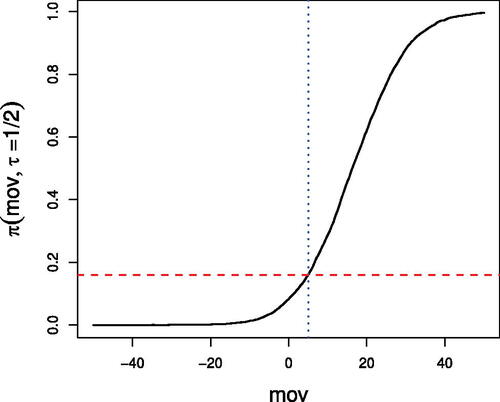
To provide further intuition for the use of conformal win probability, consider a women’s basketball game between home team South Carolina and away team Oregon State, two highly ranked teams during the 2019–2020 season (see Section 4 for more results related to the top women’s teams). For a specific MOV for this match-up, for example, a MOV of five, ${\pi }_w(5,\tau )$ is a probability estimate of the event $y_{n+1}\le 5$, which represents a MOV of less than or equal to five. Additionally, an estimate for the probability that South Carolina wins, that is, the MOV is greater than zero, is $1-{\pi }_w(0,\tau )$.

Figure 2 shows the MOV conformal predictive distribution for South Carolina versus Oregon State for the 2019–2020 season. This distribution has jumps that are too small to be visible. Thus, the distribution is nearly continuous. It is straightforward to reassign probability so that the support of the conformal predictive distribution lies entirely on nonzero integers to match the MOV distribution. However, our reassignment does not affect our win probability estimate, so we omit the details here.

Fig. 2 MOV conformal predictive distribution for South Carolina versus Oregon State with $\tau =1/2$ using regular season data from 2019 to 2020 NCAA women’s basketball season. The blue dotted line identifies a MOV for South Carolina of 5, that is, South Carolina (home) beating Oregon State (away) by five points, with $\pi (5,1/2)=0.160$ identified by the red dashed line.

With the additional assumptions of mean-zero, independent, normally distributed error terms under (16), the probability construction shown in (14) becomes (18) $$\mathbb{P}(y_{\mathit{uvw}}>0)=1-F_{t,n_w-p}\left(\frac{-{\widehat{y}}_{\mathit{uvw}}}{\widehat{\sigma }\sqrt{1+x{\prime }_{\mathit{uvw}}{(X_{w-1}^{\prime }{X}_{w-1})}^{-1}{x}_{\mathit{uvw}}}}\right),$$(18) where X_w is the matrix of covariates up to and including period w.

For logistic regression, we could instead assume (19) $$\hspace{0.17em}\log \hspace{0.17em}\left(\frac{p_{\mathit{uvw}}}{1-p_{\mathit{uvw}}}\right)=x_{\mathit{uvw}}^{\prime }\beta ,$$(19) where p_uvw is the probability that y_uvw is greater than to zero. Then, p_uvw is the probability that home team u wins against away team v in period w. Similar approaches to (19) are seen in Bradley and Terry (1952) and Lopez and Matthews (2015). The interpretation for ${\theta }_u-{\theta }_v$ under model (19) is no longer the strength difference between teams u and v in terms of MOV, but rather the log-odds of a home team victory when home team u plays away team v at a neutral site. As in linear regression, the rank order of the estimates of the θ parameters obtained by logistic regression provides a ranking of the teams.

Note that MOV predictions associated with conformal win probability using model (16) are identical to those for our GMMNE; only the approach to translate the predicted MOV to win probability differs. Additionally, logistic regression does not provide predicted MOV. Thus, we focus on the comparison of win probabilities rather than predicted MOV for these three methods.

3.3.1 Potential Betting Scenario

The focus on win probabilities can also be extended to a betting scenario. In this article, the event probability of interest is a win (or loss) for a specific team, which corresponds to a “moneyline” bet in sports betting, that is, betting on a specific team to win a game. Another type of bet is the “spread” bet, which accounts for differences in the strengths of two teams, either through the adjustment of a point spread or the odds associated with a particular team. The spread is chosen by bookmakers so that the total amount of money bet on the spread of the favorite is near that bet against favorite (as opposed to being representative of, say, the expected margin of victory). We can use conformal win probabilities (or any of the other competing methodologies discussed) in order to determine whether to bet on the favorite or the underdog in a spread bet. For conformal win probabilities specifically, calculating $1-\pi (-s,1/2)$, where s is the spread for a game of interest, generates an estimate of the probability that the MOV (favorite score–underdog score) will be greater than–s.

3.3.2 Discussion on Other Rating Methods

In later sections, we compare the ratings generated using the Harville method to other rating methods, including Associated Press (AP), NCAA Evaluation Tool (NET), KenPom (KP), Ratings Percentage Index (RPI) and College Sports Madness (CSM). While AP is subjective, NET, KP, and CSM are proprietary, with only some elements of their construction made public. Of the rating methods we compare to, RPI is the only approach where the construction is known.

In contrast to RPI, while the main components of NET are known to the public, that is, team value index and net efficiency, the inherent construction of the rankings is not. Thus, we can neither reproduce the NET rankings from recent seasons nor compute them for seasons prior to 2018. KP and CSM ratings suffer from the same lack of transparency.

The lack of transparency for NET, KP and CSM rating methods is one reason we chose the Harville method as our main approach of interest. Additionally, NET rankings have no inherent win probability associated with the respective ranks of two teams playing; we gain a probabilistic interpretation of margin of victory, through win probability, with the three approaches we use in this work, that is, a linear model with normal errors, logistic regression, and conformal win probability. We note win probabilities based on KP ratings are constructed under the assumption of normality of the expected margin of victory, with a fixed standard deviation of 11, which is not unlike our linear model with normal errors.

We point the interested reader to Jacobs (2017), Malloy (2023), and Pomeroy (2014) for discussions on the construction of RPI, NET, and KP rankings, respectively. Additionally, Barrow et al. (2013) provides a thorough comparison of a collection of ranking methods across multiple seasons for multiple sports.

Another reason for the selection of the Harville method is a product of our dataset. While richer datasets, for example, ones including field goal percentage, three-point percentage, and offensive efficiency, could be obtained for some previous seasons, we chose to construct a dataset, for many games and seasons, with just the two teams playing and the MOV for the home team. The methods we consider in our article are well-suited for this MOV dataset. Differences between the ranks associated with the Harville method and NET can be attributed to different information being used within each ranking approach.

4 Application to March Madness

We first provide exploration of the 2019–2020 NCAA DI basketball season, to include the canceled 2020 tournaments. Estimates of team strengths constructed from regular season data for the top ten women’s and men’s teams during the 2019–2020 season are shown in Tables 1 and 2, respectively. Additional 2019–2020 rankings from different sources are included for comparison; the additional rankings include Associated Press (AP), NCAA Evaluation Tool (NET), KenPom (KP), Ratings Percentage Index (RPI) and College Sports Madness (CSM).

Table 1 Top 10 NCAA women’s teams for 2019–2020 season.

Team	Estimated strength	Rank	AP	RPI	CSM
Oregon	42.42	1	2	2	2
Baylor	41.92	2	3	4	4
South Carolina	40.18	3	1	1	1
Maryland	39.29	4	4	3	6
Connecticut	36.79	5	5	4	3
Stanford	29.54	8	6	6	7
Mississippi St.	28.93	7	9	10	12
Louisville	28.11	8	6	7	6
Indiana	27.48	9	20	14	19
Oregon State	26.24	10	14	20	17

Table 2 Top 10 NCAA men’s teams for 2019–2020 season.

Team	Estimated strength	Rank	AP	NET	KP
Kansas	24.96	1	1	2	1
Gonzaga	22.87	2	2	1	2
Duke	22.22	3	11	6	5
Michigan State	21.09	4	9	7	7
Baylor	20.23	5	5	5	3
Arizona	19.27	6	–	14	19
San Diego State	18.87	7	6	4	6
Ohio State	18.81	8	19	16	8
Dayton	18.37	9	3	3	4
West Virginia	17.92	10	24	17	10

The large difference between strengths for the top men’s and women’s teams is due to the difference in teams parity between the two leagues, that is, the gap in strength between the stronger and weaker women’s teams is much larger than the gap between the stronger and weaker men’s teams. Differences in team ranks between ranking systems can be attributed to subjectivity, for example, or the use of different information, for example, RPI, NET, and KP.

The remainder of this section is dedicated to constructing probabilities of making the March Madness field and tournament win probabilities for the canceled 2019–2020 tournaments. We follow this discussion with a comparison of the win probability methods outlined in Section 3 using our historical dataset based on the 12 seasons from 2011–2012 to 2022–2023. The dataset used was compiled from two sources: masseyratings.com and ncaa.com. We include sample sizes for the training (regular season games) and validation (post-season games) datasets in Table 3.

Table 3 Training and validation set sample sizes spanning 2011–2012 and 2022–2023 seasons.

		Season
		2011–2012	2012–2013	2013–2014	2014–2015	2015–2016	2016–2017	2017–2018	2018–2019	2019–2020	2020–2021	2021–2022	2022–2023
Women	Train	4247	4336	4289	4745	4761	4785	4758	4800	4803	2957	4612	4927
	Validation	358	319	369	465	494	475	491	486	352	425	504	575
Men	Train	4750	4842	4802	4831	4836	4861	4895	4967	4972	3272	4824	5079
	Validation	501	502	479	541	549	546	545	552	300	455	568	583

4.1 Probabilities of Making March Madness Field for 2019–2020 Season

Following the cancellation of the 2020 NCAA basketball post-season, there were 20 men’s and 18 women’s automatic bids still undecided. Knowing the results of the (partially) completed conference tournaments allows for estimation of the probabilities of making the March Madness field as outlined in Section 2.2. We use regular season data as well as conference tournament progress to update every team’s chances of making the tournament at the time of cancellation. We include the tournament winners of completed conference tournaments for NCAA women’s basketball in supplementary materials. These teams have probability 1 of making the March Madness field.

With the additional information provided by the outcomes of the completed conference tournaments, there are five different situations for teams as it relates to making the March Madness tournament:

1. A team has already made the tournament.

2. To make the tournament, a team must win their conference tournament or rely on few teams ranked below them winning their respective conference tournament.

3. To make the tournament, a team has already been eliminated from their conference tournament and relies on few teams ranked below them winning their respective conference tournaments.

4. A team must win their conference tournament to make the tournament.

5. A team cannot make the tournament.

Table 4 shows the situations for women’s teams ranked from 33 to 64. Recall that due to our simplified selection process, teams ranked from 1 to 32 have already made the tournament.

Table 4 Situations for women’s bubble teams.

Situation	Teams
1	Texas, Alabama, Arizona St., Missouri St., TCU,
	Drake, James Madison, Oklahoma St.
2	Kansas St.
3	LSU, Marquette, North Carolina
4	Texas Tech, West Virginia, Oklahoma
5	all other bubble teams

When using the rankings constructed with regular season data and model (16), the Big 12 conference tournament was the only undecided tournament involving bubble teams, resulting in Kansas State being the sole team in Situation 2 and Texas Tech, West Virginia and Oklahoma as the only teams in Situation 4. Table 5 shows the March Madness tournament field probabilities for teams in Situations 2, 3, and 4, constructed with (8) and conformal win probability.

Table 5 Probabilities of making NCAA tournament field for women’s bubble teams for 2019–2020 season.

Team	Situation	Overall rank	Probability
LSU	3	41	>0.999
Marquette	3	42	0.989
Kansas St.	2	43	0.873
North Carolina	3	44	0.456
Texas Tech	4	50	0.003
West Virginia	4	52	0.004
Oklahoma	4	62	<0.001

While not listed in Table 5, there is a large number of women’s teams ranked below 64 that also fall into Situation 4. Probabilities of making the tournament for the men’s teams in Situations 2, 3, and 4 are shown in supplementary materials.

4.2 March Madness Win Probabilities

Even with the results of the completed conference tournaments, the number of potential tournament brackets remains extremely large. Thus, we forgo enumeration of all potential brackets and instead focus on three exemplar brackets and three expert brackets to generate March Madness win probabilities. We represent two extremes; Bracket 1 maximizes tournament parity by including the strongest remaining team from each conference tournament bracket, while Bracket 2 includes the weakest remaining team. Bracket 3 is constructed by randomly selecting teams based on their conference tournament win probabilities. For each of Bracket 1, 2, and 3, we use the S-curve method (NCAA 2021) to assign teams in the field to each bracket position as detailed in supplementary materials. We compare these brackets, and the March Madness win probabilities for the top teams included in these brackets, to those generated by subject matter experts.

We include projected women’s brackets from basketball expert Michelle Smith (Northam 2020), College Sports Madness (2020), and RealTimeRPI.com (2020). Table 6 shows the different bracket win probabilities for the top ten women’s teams, ranked using the ranking method outlined in Section 3.3. Exemplar bracket results for the men’s 2019-2020 season are included in supplementary materials; we also include results for the brackets generated by NCAA basketball experts Andy Katz (Staats and Katz 2020), Joe Lunardi (Lunardi 2020) and Jerry Palm (Palm 2020). All subject matter expert brackets for the 2019–2020 tournaments are publicly available. Figure 3 shows win probabilities across the expert generated brackets and a comparison of cumulative NCAA tournament win probabilities across brackets for the top ten women’s teams. A similar figure for the top ten men’s teams is included in supplementary materials.

Fig. 3 Expert bracket win probabilities (left) and cumulative win probabilities (right) for top 10 women’s teams during the 2019–2020 season.

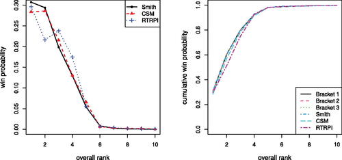
Table 6 March Madness win probabilities given exemplar brackets for top ranked women’s teams.

Team	Bracket 1	Bracket 2	Bracket 3	Smith	CSM	RTRPI
Oregon	0.308	0.308	0.308	0.307	0.284	0.296
Baylor	0.295	0.295	0.295	0.294	0.286	0.216
South Carolina	0.197	0.197	0.197	0.199	0.215	0.239
Maryland	0.123	0.124	0.124	0.130	0.130	0.175
Connecticut	0.057	0.057	0.057	0.055	0.065	0.056
Stanford	0.007	0.007	0.007	0.008	0.007	0.007
Mississippi St.	0.004	0.004	0.004	0.003	0.003	0.005
Louisville	0.002	0.002	0.002	0.001	0.003	0.002
Indiana	0.002	0.002	0.002	0.001	0.002	0.001
Oregon St.	0.001	0.001	0.001	0.000	0.001	0.001

In general, tournament win probabilities do not change drastically across brackets. However, there are some noteworthy differences. Specifically, the tournament win probability for Baylor, the second-highest ranked team with respect to our ranking, drops to 0.216 with the RTRPI expert bracket, compared to 0.294 and 0.286 for the Smith and CSM brackets, respectively. Additionally, the tournament win probability for South Carolina increases to 0.239 with the RTRPI bracket; their win probability is 0.199 and 0.215 for the Smith and CSM brackets, respectively. Figure 4 shows round-by-round win probabilities for Baylor and South Carolina for each expert bracket.

Fig. 4 Round-by-round win probabilities for Baylor and South Carolina constructed with expert brackets from Michelle Smith (top left), College Sports Madness (top right) and RTRPI (bottom middle). The values shown indicate the probabilities of a team moving on from a particular round.

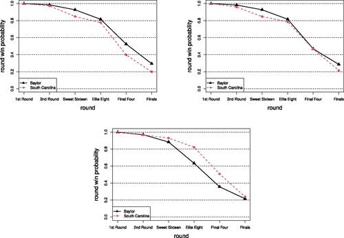
We see that Baylors’s RTRPI round-by-round win probability becomes lower than South Carolina’s during the Sweet Sixteen, dropping to 0.884, compared to South Carolina’s 0.929. The largest decrease occurs during the Elite Eight, where Baylor’s probability of moving on from the Elite Eight (under the RTRPI bracket) is 0.633, compared to South Carolina’s 0.821. This is due to Connecticut’s placement in the same region as Baylor, with each team seeded as the 1-seed and 2-seed, respectively. In the other expert brackets, Connecticut was placed in the same region as Maryland, which keeps the round-by-round win probabilities for these two teams relatively stable.

4.3 Win Probability Calibration

While our discussion has explored the 2019–2020 NCAA D1 season and canceled tournaments, we also wish to assess the effectiveness of conformal win probability more broadly. In order to assess conformal win probability estimates, as well as the other win probability methods outlined in Section 3, we compare estimates for previous NCAA basketball seasons, including the shortened 2019–2020 season. We use the regular season games to estimate the team strengths and then construct win probabilities for each game of post-season play.

Ideally, the estimated probability for an event occurring should be calibrated. A perfectly calibrated model is one such that (20) $${\mathrm{E}}_{\widehat{p}}\left[\right|\mathbb{P}(\widehat{z}=z|\widehat{p}=p)-p|]=0,$$(20) where z is an observed outcome, $\widehat{z}$ is the predicted outcome, $\widehat{p}$ is a probability estimate for the predicted outcome, and p is the true outcome probability (Guo et al. 2017). In the NCAA basketball case, (20) implies that if we inspect, say, each game with an estimated probability of 40% for home team victory, we should expect a home team victory in 40% of the observed responses. We can assess calibration in practice by grouping similarly valued probability estimates into a single bin and then calculating the relative frequency of home team victories for observations within each bin. For visual comparison of calibration, Figure 5 shows a reliability plot for the win probability estimates generated using the methods outlined in Section 3 with bin intervals of width 0.025.

Fig. 5 Empirical calibration comparison for NCAA women’s and men’s basketball for 2011–2012 to 2022–2023 post-seasons for methods outlined in Section 3.

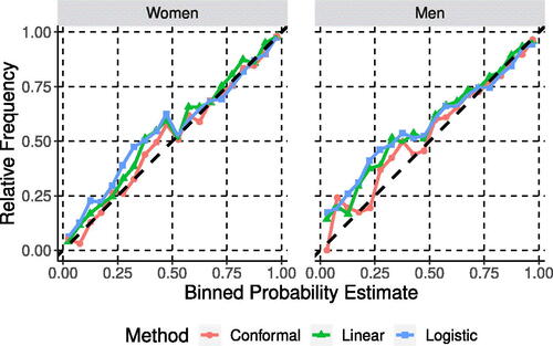
From Figure 5 we can see that while the methods are comparable for higher win probability estimates, the conformal win probability approach is much better calibrated for lower win probability estimates. A majority of observed relative frequencies for conformal win probabilities fall closer to the dotted line, signifying better calibration than the other two methods.

To provide a numerical summary of calibration, we compare the win probability estimation approaches from Section 3 using log-loss; the log-loss for a single observation is defined as the negative log-likelihood of the independent Bernoulli trial evaluated at the win probability estimate. The log-loss for a set of estimates is a sum of terms of the form $-z\hspace{0.17em}\log \hspace{0.17em}(\widehat{p})+(1-z)\hspace{0.17em}\log \hspace{0.17em}(1-\widehat{p})$, with one such term for each game. This log-loss incorporates a loss for each individual win probability estimate rather than a group of binned estimates. Figure 6 shows the relative log-loss, that is, the ratio of the log-loss for one method to the minimum log-loss across all methods, broken up by season and league. We include raw log-loss plots in supplementary materials.

Fig. 6 Relative log-loss comparison for NCAA women’s and men’s basketball for win probability estimates associated with 2011–2012 to 2022–2023 post-seasons for methods outlined in Section 3.

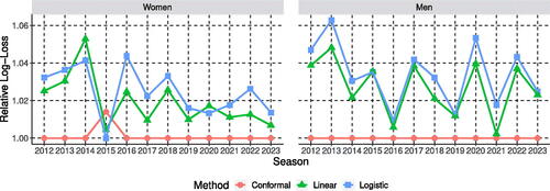
In all but one of the year-league combinations, conformal win probabilities result in lower log-loss than the other two methods. It should be noted however that log-loss for the other methods was within five percent of conformal win probability log-loss for most year-league combinations. Table 7 shows the results for the three win probability methods within each league when log-losses are summed across all 12 seasons. We also include accuracy results (proportion of game outcomes correctly predicted) for each method by league in Table 8.

Table 7 Relative log-loss for NCAA men’s and women’s basketball win probability estimates by league.

League	Conformal	Linear	Logistic
Women	1.000	1.016	1.023
Men	1.000	1.026	1.033

Table 8 Proportion of games corrected predicted for 2011–2023 seasons.

League	Conformal	Linear	Logistic
Women	0.751	0.743	0.743
Men	0.713	0.699	0.699
Overall	0.731	0.719	0.719

4.4 Comparison to Publicly Available Methods

In an effort to further compare conformal win probability based on model (16) to other modeling approaches not included in this article, we point the interested reader to Bunker and Susnjak (2022), which provides a survey of model accuracy results for a suite of methods for generating game-by-game win probabilities in basketball. Bunker and Susnjak (2022) consider methods developed for both NCAA and National Basketball Association (NBA) games. Reported accuracies on datasets different from ours range from 0.67 to 0.83 for methods that include naive Bayes, logistic regression, neural networks and decision trees. Most of the methods considered by Bunker and Susnjak (2022) use richer feature sets than our approach, which only uses only the home team and away team identities as predictors. Details of these other methods can be found in Thabtah, Zhang, and Abdelhamid (2019), Ivanković et al. (2010), Loeffelholz, Bednar, and Bauer (2009), Shi, Moorthy, and Zimmermann (2013), Zdravevski and Kulakov (2009), Cao (2012), and Miljković et al. (2010).

As another avenue of comparison, we also use results from recent Kaggle March Machine Learning Mania (KMMLM) competitions. We first compare our results using the conformal win probability approach outlined in this article to the KMMLM leaderboards for the 2015 to 2022 iterations. These results are shown in Table 9, with better performing models having a higher percentile.

Table 9 log-loss performance of conformal win probabilities based on model (16) to Kaggle March Madness leaderboards for men’s March Madness, with higher percentiles indicating better performance.

Season	2015	2016	2017	2018	2019	2020	2021	2022
log-loss	0.516	0.570	0.497	0.716	0.469	–	0.631	0.670
Percentile	0.458	0.697	0.739	0.193	0.816	–	0.492	0.405
# of Submissions	345	598	441	934	863	–	707	930

Based in the results in Table 10, conformal win probabilities generated with the Harville method do not seem to be competitive when compared to other KMMLM models. This can be partially attributed to use of additional covariates with in these models.

Table 10 Kaggle methods used for comparison to conformal win probability.

Kaggle User	League	Method	Repository
raddar (raddar 2018)	NCAAW/NCAAM	XGBoost	https://github.com/fakyras/ncaa_women_2018
Gdub (Wierzbicki 2019)	NCAAM	Logistic Regression	https://github.com/gjwierz/NCAA_Kaggle_2019
Sapper (Turner 2021)	NCAAM	Random Forest	https://github.com/dusty-turner/ncaa_tournament_2021_beat_navy

Thus far, we have considered the performance of conformal win probabilities derived from the relatively simple linear model in (16). However, as noted in Section 3.1, the conformal approach can be used with any MOV prediction method to obtain win probability estimates. We now seek to determine if strong performing KMMLM approaches can be improved by conformal inference.

We consider the subset of KMMLM models from the men’s and women’s competition that meet the following criteria: (a) occurred within the last five most recent iterations of the competition, (b) finished the competition in first or second place, and (c) had minimum viable code to reproduce their results completely in R. The three publicly available solutions that met this criteria, the league to which they were applied (men and/or women) and the code repository are shown in Table 10.

Kaggle user raddar provided the top solution for the 2018 women’s iteration of KMMLM through the use of XGBoost (Chen and Guestrin 2016). Additionally, nonparametric regression was used to transform expected margins of victory generated using XGBoost to win probabilities; we included additional adjustments to constrain the output from the nonparametric regression to the interval (0, 1). We note that this solution has been used with great success for both the men’s and women’s tournament in more recent years, with many top performers referencing this model as their starting point. Gdub provided the second place solution in the 2019 iteration of the KMMLM men’s competition through logistic regression with eight covariates, which include seed differences, adjusted offensive and defensive efficiency, strength of schedule, team ranks, turnovers and free-throw percentage. We use the same covariates, but adjust the model to estimate MOV, as opposed to generating probability estimates explicitly; conformal win probability estimates were then constructed based on the fitted predictors as described in Section 3. The third model of interest, provided by Sapper, is a random forest-based approach. We use each of these methods to generate win probabilities for the 2015 to 2023 tournament iterations. We then compare those results to the same methods but with win probabilities determined via conformal inference.

A comparison of conformal win probability to the other methods for the 2015–2023 women’s and men’s tournaments (with respect to log-loss) are shown in Tables 11 and 12, respectively. We note that the raddar model was readily applicable to both NCAAW and NCAAM tournaments, but the GDub and Sapper models were only applicable to the NCAAM tournaments. We lack an application of the Sapper model to the 2023 iteration of the men’s tournament due to unavailable data.

Table 11 log-loss comparison of conformal win probabilities to well performing KMMLM competition models for 2015–2023 NCAAW March Madness tournaments.

Kaggle User	Model	2015	2016	2017	2018	2019	2021	2022	2023
raddar	Base	0.3712	0.5143	0.4387	0.4342	0.3658	0.4764	0.4652	0.4976
	Conformal	0.3873	0.5076	0.4379	0.4314	0.3763	0.4619	0.4655	0.4893

Table 12 log-loss comparison of conformal win probabilities to well performing KMMLM competition models for 2015–2023 NCAAM March Madness tournaments.

Kaggle User	Model	2015	2016	2017	2018	2019	2021	2022	2023
Gdub	Base	0.4970	0.5931	0.5244	0.6049	0.5033	0.6637	0.5780	0.6509
	Conformal	0.4983	0.5890	0.5078	0.6018	0.5103	0.6386	0.5847	0.6370
raddar	Base	0.5108	0.5871	0.4996	0.6741	0.4884	0.6160	0.6481	0.7031
	Conformal	0.5212	0.5809	0.5092	0.6052	0.5020	0.6024	0.6304	0.6416
Sapper	Base	0.5808	0.5611	0.5882	0.6022	0.4605	0.6001	0.7182	–
	Conformal	0.5318	0.5644	0.5147	0.6001	0.4951	0.6188	0.6274	–

In Tables 11 and 12, we underline the best performing method for each pairwise comparison between a Kaggle top performer and its conformal counterpart. We also bold the results for the best performing method overall within each league. For each combination of league and Kaggle method, conformalization led to an improvement over the original method for a majority of seasons.

5 Conclusion

The 2020 March Madness cancellation was disappointing for many fans and athletes. We explored win probabilities related to the NCAA tournament, delivering closed-form calculations for probabilities of making the tournament, given a set of team strengths estimated from game outcomes. We also identified the most likely winners of the men’s and women’s tournaments. We introduced conformal win probabilities, which compared favorably with win probabilities derived from logistic and linear regression assuming normally distributed, independent, mean-zero errors. While we focused primarily on conformal win probabilities derived from a relatively simple linear model, we also showed that more complex methods can be improved via conformal inference.

One simplification we use in this article is that estimated team strength does not change following the regular season. Thus, we eliminate the potential for teams to receive a higher (or lower) overall rank based on their conference tournament performance. While this simplifies the analysis, allowing for teams to move up or down in rank might more closely match the March Madness selection committee’s actual process. We use “full” conformal predictive distributions to generate our conformal win probabilities. It would be interesting to see how variants of conformal predictive distributions, for example, split or Mondrian, perform as well.

Acknowledgments

The authors would like to thank the Editor, Associate Editor and two referees for their careful reviews of the manuscript and insightful comments and suggestions.

Supplementary Materials

We provide additional exploration of the 2019–2020 March Madness tournament in supplementary materials. The supplementary materials include discussion related to the men’s tournament, including results with the inclusion of a First Four, as well as a set of exemplar and expert brackets, and tournament win probability estimates constructed based on conformal win probabilities. We also include further comparison of each of the win probability methods we focused on to a version of the Elo method (Elo 1961).

Disclosure Statement

No potential competing interests were reported by the author(s).

Additional information

Funding

This research was supported in part by the US National Science Foundation under grant HDR:TRIPODS 19-34884.

References

- Asif, M., and McHale, I. G. (2016), “In-Play Forecasting of Win Probability in One-Day International Cricket: A Dynamic Logistic Regression Model,” International Journal of Forecasting, 32, 34–43. DOI: 10.1016/j.ijforecast.2015.02.005.
- Barnard, G. (1989), “On Alleged Gains in Power from Lower p-values,” Statistics in Medicine, 8, 1469–1477. DOI: 10.1002/sim.4780081206.
- Barrow, D., Drayer, I., Elliott, P., Gaut, G., and Osting, B. (2013), “Ranking Rankings: An Empirical Comparison of the Predictive Power of Sports Ranking Methods,” Journal of Quantitative Analysis in Sports, 9, 187–202. DOI: 10.1515/jqas-2013-0013.
- Bassett, G. W. (2007, “Quantile Regression for Rating Teams,” Statistical Modelling, 7, 301–313.
- Bradley, R. A., and Terry, M. E. (1952), “Rank Analysis of Incomplete Block Designs: I. The Method of Paired Comparisons,” Biometrika, 39, 324–345. DOI: 10.2307/2334029.
- Bunker, R., and Susnjak, T. (2022), “The Application of Machine Learning Techniques for Predicting Match Results in Team Sport: A Review,” Journal of Artificial Intelligence Research, 73, 1285–1322. DOI: 10.1613/jair.1.13509.
- Cao, C. (2012), “Sports Data Mining Technology Used in Basketball Outcome Prediction.” Master thesis, Technological University Dublin, pp. 1–106.
- Carlin, B. P. (2005), “Improved NCAA Basketball Tournament Modeling via Point Spread and Team Strength Information,” in Anthology of Statistics in Sports, pp. 149–153, Philadelphia, PA: SIAM.
- Chen, T., and Guestrin, C. (2016). “Xgboost: A Scalable Tree Boosting System,” in Proceedings of the 22nd ACM SIGKDD International Conference on Knowledge Discovery and Data Mining, pp. 785–794.
- College Sports Madness. (2020), “Women’s Basketball Bracketology,” available at https://www.collegesportsmadness.com/womens-basketball/bracketology
- Edwards, C. T. (1991), “The Combinatorial Theory of Single-Elimination Tournaments,” PhD thesis, Montana State University-Bozeman, College of Letters & Science.
- Elfrink, T. (2018), Predicting the Outcomes of MLB Games with a Machine Learning Approach, Amsterdam: Vrije Universiteit.
- Elo, A. E. (1961), “The USCF Rating System,” Chess Life, 160–161.
- Gammerman, A., Vovk, V., and Vapnik, V. (1998), “Learning by Transduction,” in Proceedings of the Fourteenth Conference on Uncertainty in Artificial Intelligence, pp. 148–155.
- Gramacy, R. B., Jensen, S. T., and Taddy, M. (2013), “Estimating Player Contribution in Hockey with Regularized Logistic Regression,” Journal of Quantitative Analysis in Sports, 9, 97–111. DOI: 10.1515/jqas-2012-0001.
- Guo, C., Pleiss, G., Sun, Y., and Weinberger, K. Q. (2017), “On Calibration of Modern Neural Networks,” in International Conference on Machine Learning, pp. 1321–1330, PMLR.
- Harville, D. (1977), “The Use of Linear-Model Methodology to Rate High School or College Football Teams,” Journal of the American Statistical Association, 72, 278–289. DOI: 10.1080/01621459.1977.10480991.
- Harville, D. A., and Smith, M. H. (1994), “The Home-Court Advantage: How Large Is It, and Does It Vary From Team to Team?” The American Statistician, 48, 22–28. DOI: 10.2307/2685080.
- Horvat, T., and Job, J. (2020), “The Use of Machine Learning in Sport Outcome Prediction: A Review,” Wiley Interdisciplinary Reviews: Data Mining and Knowledge Discovery, 10, e1380.
- Ivanković, Z., Racković, M., Markoski, B., Radosav, D., and Ivković, M. (2010), “Analysis of Basketball Games Using Neural Networks,” in 2010 11th International Symposium on Computational Intelligence and Informatics (CINTI), pp. 251–256, IEEE. DOI: 10.1109/CINTI.2010.5672237.
- Jacobs, J. (2017), “How to Game the Rating Percentage Index (RPI) in Basketball,” available at https://squared2020.com/2017/03/10/how-to-game-the-rating-percentage-index-rpi-in-basketball/
- Kaplan, E. H., and Garstka, S. J. (2001), “March Madness and the Office Pool,” Management Science, 47, 369–382. DOI: 10.1287/mnsc.47.3.369.9769.
- Lancaster, H. O. (1961), “Significance Tests in Discrete Distributions,” Journal of the American Statistical Association, 56, 223–234. DOI: 10.1080/01621459.1961.10482105.
- Lawless, J., and Fredette, M. (2005), “Frequentist Prediction Intervals and Predictive Distributions,” Biometrika, 92, 529–542. DOI: 10.1093/biomet/92.3.529.
- Lee, A. (1999), “Applications: Modelling Rugby League Data via Bivariate Negative Binomial Regression,” Australian & New Zealand Journal of Statistics, 41, 141–152. DOI: 10.1111/1467-842X.00070.
- Lei, J., G’Sell, M., Rinaldo, A., Tibshirani, R. J., and Wasserman, L. (2018), “Distribution-Free Predictive Inference for Regression,” Journal of the American Statistical Association, 113, 1094–1111. DOI: 10.1080/01621459.2017.1307116.
- Liebscher, S., and Kirschstein, T. (2017), “Predicting the Outcome of Professional Darts Tournaments,” International Journal of Performance Analysis in Sport, 17, 666–683. DOI: 10.1080/24748668.2017.1372162.
- Lindsey, G. R. (1961), “The Progress of the Score during a Baseball Game,” Journal of the American Statistical Association, 56, 703–728. DOI: 10.1080/01621459.1961.10480656.
- Liu, Q., Zhuang, Y., and Wan, F. (2016), “A New Model for Analyzing the Win Probability and Strength of the Two Sides of the Table Tennis Match,” in First International Conference on Real Time Intelligent Systems, pp. 52–59, Springer.
- Lock, D., and Nettleton, D. (2014), “Using Random Forests to Estimate Win Probability Before Each Play of an NFL Game,” Journal of Quantitative Analysis in Sports, 10, 197–205. DOI: 10.1515/jqas-2013-0100.
- Loeffelholz, B., Bednar, E., and Bauer, K. W. (2009), “Predicting NBA Games Using Neural Networks,” Journal of Quantitative Analysis in Sports, 5. DOI: 10.2202/1559-0410.1156.
- Lopez, M. J., and Matthews, G. J. (2015), “Building an NCAA Men’s Basketball Predictive Model and Quantifying Its Success,” Journal of Quantitative Analysis in Sports, 11, 5–12. DOI: 10.1515/jqas-2014-0058.
- Lunardi, J. (2020), “Bracketology with Joe Lunardi,” available at http://www.espn.com/mens-college-basketball/bracketology
- Maher, M. J. (1982), “Modelling Association Football Scores,” Statistica Neerlandica, 36, 109–118. DOI: 10.1111/j.1467-9574.1982.tb00782.x.
- Malloy, G. (2023), “College Basketball’s NET Rankings, Explained: How Data Science Drives March Madness,” available at https://towardsdatascience.com/college-basketballs-net-rankings-explained-25faa0ce71ed
- Miljković, D., Gajić, L., Kovačević, A., and Konjović, Z. (2010), “The Use of Data Mining for Basketball Matches Outcomes Prediction,” in IEEE 8th International Symposium on Intelligent Systems and Informatics, IEEE, pp. 309–312.
- NCAA. (2021), “How the Field of 68 Teams is Picked for March Madness,” available at https://www.ncaa.com/news/basketball-men/article/2021-01-15/how-field-68-teams-picked-march-madness
- Niemi, J. B., Carlin, B. P., and Alexander, J. M. (2008), “Contrarian Strategies for NCAA Tournament Pools: A Cure for March Madness?” Chance, 21, 35–42. DOI: 10.1080/09332480.2008.10722884.
- Northam, M. (2020), “The NCAA Women’s Basketball Bracket, Projected 6 Days from Selections,” available at https://www.ncaa.com/news/basketball-women/article/2020-03-10/ncaa-womens-basketball-bracket-projected-6-days-selections
- Palm, J. (2020), “Bracketology,” available at https://www.cbssports.com/college-basketball/bracketology/
- Pifer, N. D., DeSchriver, T. D., Baker III, T. A., and Zhang, J. J. (2019), “The Advantage of Experience: Analyzing the Effects of Player Experience on the Performances of March Madness Teams,” Journal of Sports Analytics, 5, 137–152. DOI: 10.3233/JSA-180331.
- Pomeroy, K. (2014), “Ratings Methodology Update,” available at https://kenpom.com/blog/ratings-methodology-update/
- raddar. (2018), “ncaa_women_2018,” available at https://github.com/fakyras/ncaa/_women/_2018
- RealTimeRPI.com. (2020), “RealTimeRPI.com Bracket Projections - Women’s Basketball,” available at http://realtimerpi.com/bracketology/bracketology/_Women.html
- Robberechts, P., Van Haaren, J., and Davis, J. (2019), “Who Will Win It? An In-Game Win Probability Model for Football,” arXiv preprint arXiv:1906.05029.
- Santos-Fernandez, E., Wu, P., and Mengersen, K. L. (2019), “Bayesian Statistics Meet Sports: A Comprehensive Review,” Journal of Quantitative Analysis in Sports, 15, 289–312. DOI: 10.1515/jqas-2018-0106.
- Schwertman, N. C., Schenk, K. L., and Holbrook, B. C. (1996), “More Probability Models for the NCAA Regional Basketball Tournaments,” The American Statistician, 50, 34–38. DOI: 10.2307/2685041.
- Semenov, A., Romov, P., Korolev, S., Yashkov, D., and Neklyudov, K. (2016), “Performance of Machine Learning Algorithms in Predicting Game Outcome from Drafts in Dota 2,” in International Conference on Analysis of Images, Social Networks and Texts, pp. 26–37, Springer.
- Shi, Z., Moorthy, S., and Zimmermann, A. (2013), “Predicting NCAAB Match Outcomes Using ML Techniques–Some Results and Lessons Learned,” in ECML/PKDD 2013 Workshop on Machine Learning and Data Mining for Sports Analytics.
- Soto Valero, C. (2016), “Predicting Win-Loss Outcomes in MLB Regular Season Games—A Comparative Study Using Data Mining Methods,” Journal homepage: available at http://iacss.org/index.php?id, 15.
- Staats, W., and Katz, A. (2020), NCAA Predictions: Projections for the 2020 Bracket,” available at https://www.ncaa.com/news/basketball-men/article/2020-02-28/ncaa-predictions-projections-2020-bracket-andy-katz
- Stern, H. (1991), “On the Probability of Winning a Football Game,” The American Statistician, 45, 179–183. DOI: 10.2307/2684286.
- Thabtah, F., Zhang, L., and Abdelhamid, N. (2019), “NBA Game Result Prediction Using Feature Analysis and Machine Learning,” Annals of Data Science, 6, 103–116. DOI: 10.1007/s40745-018-00189-x.
- Trono, J. A. (2010), “Rating/Ranking Systems, Post-Season Bowl Games, and the Spread,” Journal of Quantitative Analysis in Sports, 6, 1–20. DOI: 10.2202/1559-0410.1220.
- Turner, D. (2021), “ncaa_tournament_2021_beat_navy,” available at https://github.com/dusty-turner/ncaa/_tournament/_2021/_beat/_navy
- Vovk, V., Gammerman, A., and Shafer, G. (2005), Algorithmic Learning in a Random World, New York: Springer.
- Vovk, V., Shen, J., Manokhin, V., and Min-ge, X. (2019), “Nonparametric Predictive Distributions based on Conformal Prediction,” Machine Learning, 108, 445–474. DOI: 10.1007/s10994-018-5755-8.
- Wang, C.-M., Hannig, J., and Iyer, H. K. (2012), “Fiducial Prediction Intervals,” Journal of Statistical Planning and Inference, 142, 1980–1990. DOI: 10.1016/j.jspi.2012.02.021.
- Wierzbicki, G. (2019), “NCAA_Kaggle_2019,” available at https://github.com/gjwierz/NCAA/_Kaggle/_2019
- Zdravevski, E., and Kulakov, A. (2009), “System for Prediction of the Winner in a Sports Game,” in International conference on ICT innovations, pp. 55–63, Springer.
- Zimmerman, D. L., Zimmerman, N. D., and Zimmerman, J. T. (2021), “March Madness ‘Anomalies’: Are They Real, and If So, Can They Be Explained?”, The American Statistician, 75, 207–216. DOI: 10.1080/00031305.2020.1720814.