Sequential Monitoring Using the Second Generation P-Value with Type I Error Controlled by Monitoring Frequency

Abstract

The Second Generation P-Value (SGPV) measures the overlap between an estimated interval and a composite hypothesis of parameter values. We develop a sequential monitoring scheme of the SGPV (SeqSGPV) to connect study design intentions with end-of-study inference anchored on scientific relevance. We build upon Freedman’s “Region of Equivalence” (ROE) in specifying scientifically meaningful hypotheses called Pre-specified Regions Indicating Scientific Merit (PRISM). We compare PRISM monitoring versus monitoring alternative ROE specifications. Error rates are controlled through the PRISM’s indifference zone around the point null and monitoring frequency strategies. Because the former is fixed due to scientific relevance, the latter is a targettable means for designing studies with desirable operating characters. An affirmation step to stopping rules improves frequency properties including the error rate, the risk of reversing conclusions under delayed outcomes, and bias.

Keywords:

• Delayed outcomes
• Interval monitoring
• Monitoring frequency
• Pre-specified regions indicating scientific merit
• Scientific relevance
• Second Generation P-Value

1 Introduction

Most clinical trials are designed to detect a minimally scientifically meaningful effect with high probability. Despite the effort to incorporate scientific relevance, a trial may establish statistical significance without establishing scientific relevance. Establishing scientific relevance requires a trial to pre-specify scientifically relevant effects and an analysis that draws conclusions regarding these effects. The purpose of this article is to develop, investigate, and provide guidance on an interval monitoring scheme that follows trials until scientific relevance is established. In this article, we will formulate scientifically meaningful hypotheses, a novel interval monitoring scheme using the Second Generation P-Value (SGPV), and monitoring frequency mechanisms to control Type I error.

Scientifically meaningful effects are unequivocally superior or inferior to the status quo. In many settings, some effects are neither accepted as clearly superior nor inferior. Freedman, Lowe, and Macaskill (1984) call these scientifically ambiguous effects the Region of Equivalence (ROE). The ROE can exclude the point null of no difference (Freedman, Lowe, and Macaskill 1984, Figure 1), include the point null as a boundary (Hobbs and Carlin 2008, sec. 2.2), or surround the point null (Kruschke 2011). Kruschke (2018) calls a ROE that surrounds the point null a Region of Practical Equivalence (ROPE) when it includes “parameter values that are equivalent to the null value for practical purposes.” (Kruschke defines the word “equivalence” as an effect indifferent from the point null hypothesis whereas Freedman defines the word “equivalence” as an effect in which the scientific community may disagree with regarding the effect’s superiority). There is no clear consensus on how the ROE should be specified; however, concerning interval monitoring, we will demonstrate that different ROE specifications can impact trial design attributes related to sample size and error rates.

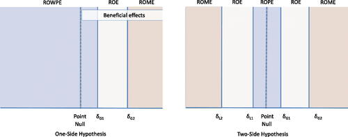
Fig. 1 Pre-Specified Regions Indicating Scientific Merit (PRISM) for one- and two-sided hypotheses. The PRISM always includes three exhaustive, non-empty, and mutually exclusive regions: a ROWPE/ROPE, a ROE, and a ROME.

The first contribution of this work is to constrain the ROE to exclude effects practically equivalent to the point null hypothesis, which creates what we call Pre-Specified Regions Indicating Scientific Merit (PRISM). This approach is similar in spirit to the original introduction of the ROE (Freedman, Lowe, and Macaskill 1984, Figure 1), though with a more explicit constraint. The constrained ROE’s complement is a ROPE surrounding the null hypothesis and a Region of Meaningful Effects (ROME). In the context of interval monitoring, we will demonstrate through simulation that PRISM monitoring reduces false discoveries as when monitoring a ROPE by itself (Kruschke 2013) though with a closed sample size. In this work, PRISM is developed to establish superiority or inferiority, without consideration of non-inferiority.

Any statistical metric can monitor the PRISM. In this work, we fashioned the Triangular Test (Anderson 1960) for likelihood ratio PRISM monitoring. However, we highlight possible discrepancies between interval estimation and the conclusions drawn from the Triangular Test’s stopping rule for scientific relevance. Though the Triangular Test is only one consideration of an alternative metric to interval monitoring, it reinforces the value of aligning stopping rules with interval estimation. No single-valued metric is sufficient to learn of the most plausible effects. An interval conveys this information.

The SGPV (Blume et al. 2018, 2019; Stewart and Blume 2019; Zuo, Stewart, and Blume 2021; Sirohi et al. 2022) is an evidence-based metric that quantifies the overlap between a finite interval I and the set of effects in a composite hypothesis H rather than a single effect as a point hypothesis. The interval includes [a, b] where a and b are real numbers such that a < b, and the length of the interval is b–a and denoted $\left|I\right|$. The overlap between the interval and the set H is $\left|I\cap H\right|$. The SGPV is calculated as $$p_H=\frac{|I\cap H|}{\left|I\right|}\times \mathrm{\text{max}}\left\{\frac{\left|I\right|}{2\left|H\right|},1\right\}.$$

The adjustment, $\mathrm{\text{max}}\left\{\frac{\left|I\right|}{2\left|H\right|},1\right\}$, is a small sample size correction—setting p_H to half of the overlap when the inferential interval overwhelms H by at least twice the length. By pre-specifying a scientifically relevant hypothesis, the SGPV brings study design transparency and bridges a gap that can exist between study design intentions and end-of-study inference regarding scientific relevance. Herein, and in the supplementary material, we compare SGPV assumptions and inference with well-established likelihood, frequentist, and Bayesian inferential metrics.

The second contribution of this work is to formalize sequential monitoring of the SGPV (SeqSGPV). SeqSGPV allows for any interval monitoring scheme of scientifically-motivated composite hypotheses. This includes, for example, “Repeated Confidence Intervals” monitoring which inverts group sequential hypothesis tests (Jennison and Turnbull 1989) and ROPE monitoring with a (1$-\alpha )$% highest density interval (Kruschke 2013). Hence, the SeqSGPV novelty is in the development of a monitoring scheme tailored to SGPV monitoring and interpretation with error control. Schemes that monitor intervals and do not adjust for frequency properties—such as unadjusted repeated 95% confidence, 95% credible, and 6.83 support intervals—need alternative means to control Type I error. Incorporating a ROPE and adjusting the monitoring frequency are two ways to reduce false discovery errors under the point null hypothesis. We consider scientific relevance fixed and the latter a targetable means for study investigators to control error rates.

As a third contribution of this work, we propose using an affirmation step to reduce error rates and estimation bias common to adaptive monitoring. Once a study meets a stopping rule criteria, the affirmation step requires the same stopping criteria to be reobserved. Dose-escalation trials have used a similar step to terminate a trial after repeatedly treating patients at the recommended maximum tolerable dose (Korn et al. 1994; Goodman, Zahurak, and Piantadosi 1995); however, we further investigate its use outside of dose-escalation trials for its ability to improve frequency properties.

Our development of SeqSGPV begins in Section 2 with a preliminary framework and notation for the PRISM and PRISM hypotheses. In Section 3, we provide SeqSGPV rules for monitoring scientifically relevant hypotheses, emphasizing PRISM hypotheses. Simulations in Section 4 investigate limiting and maximum sample size error probabilities under different ROE specifications. We evaluate the impact of different monitoring frequency strategies, including adding an affirmation step. We compare SeqSGPV PRISM monitoring to monitoring ROPE alone (Kruschke 2013) in controlling Type I error and sample size. Additionally, we compare PRISM monitoring to monitoring for any benefit (i.e., a ROE with a point null boundary as considered in Hobbs and Carlin 2008, sec. 2.2). Section 5 compares PRISM monitoring using SeqSGPV versus the Triangular Test. Section 6 applies SeqSGPV to a real-world setting and data from a randomized trial on diabetes management. We end in Section 7 with a discussion, limitations, and extensions.

2 PRISM Notation and SGPV Conclusions

For a parameter $\theta \in \Omega$, a PRISM fully divides the parameter space into three non-empty and mutually exclusive regions: ROPE, ROE, and ROME. In a two-sided hypothesis, ROPE effects lay in the set $[{\delta }_{L1},{\delta }_{G1}]$ in which ${\delta }_{L1}$ and ${\delta }_{G1}$ are practically equivalent, respectively less than or greater than the point null. Scientifically meaningful effects are of a magnitude of at least ${\delta }_{L2}$ or ${\delta }_{G2}$ which are respectively less than or greater than the point null. The remaining ROE effects reflect those in which there is scientific ambiguity regarding the effect’s superiority. In a one-sided hypothesis, the ROPE is replaced by a Region of Worse or Practically Equivalent Effects (ROWPE). When a positive effect is beneficial, the ROWPE includes effects up to ${\delta }_{G1}$; when a negative effect is beneficial ROWPE includes effects as low as ${\delta }_{L1}$ (Figure 1). Subscripts denote region boundaries. For example, ROE ${}_{({\delta }_{G1},{\delta }_{G2})}$ denotes ROE including effects within the set $({\delta }_{G1},{\delta }_{G2})$. Specifying ROE boundaries that exclude a ROPE fully specifies the PRISM.

For SeqSGPV, the two-sided hypotheses of interest are $H_{\mathit{\text{ROPE}}}:\theta \in \mathit{\text{ROPE}}$ and $H_{\mathit{\text{ROME}}}:\theta \in \mathit{\text{ROME}}$; the one-sided hypotheses of interest are similar but replace H_ROPE with $H_{\mathit{\text{ROWPE}}}:\theta \in \mathit{\text{ROWPE}}$. Given an interval, practically equivalent effects to the point null are ruled out when p_ROPE =0 whereas the data support practically equivalent null effects when p_ROPE =1. The data regarding ROPE are inconclusive when 0$<p_{\mathit{\text{ROPE}}}<$1. The interpretation is similar for a ROME hypothesis. When applied to a two-sided hypothesis, 13 ROPE and ROME conclusions may be drawn from the SGPV (Figure 2); eight ROWPE and ROPE conclusions may be drawn from a one-sided hypothesis. For sequential PRISM monitoring, we follow until either p_ROPE = 0 or p_ROME = 0 which reduces to four conclusions:

Fig. 2 Possible two-sided PRISM SGPV conclusions. Similar conclusions may be drawn from a one-sided PRISM. SeqSGPV monitors for conclusive evidence to rule out equivalent effects to the point null (p_ROPE = 0 or p_ROWPE = 0) or to rule out scientifically meaningful effects (p_ROME = 0).

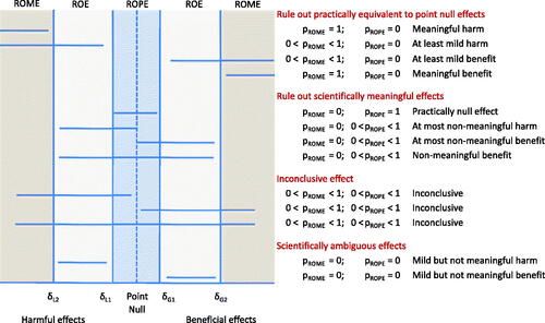
• p_ROPE = 0 & $p_{\mathit{\text{ROME}}}\ne 0$ is evidence to rule out effects practically equivalent to the point null.

• p_ROME = 0 & $p_{\mathit{\text{ROPE}}}\ne 0$ is evidence to rule out scientifically meaningful effects.

• p_ROPE = 0 & p_ROME = 0 is evidence for scientifically ambiguous effects only.

• Otherwise, the effect is of inconclusive merit.

3 Sequentially Monitoring PRISM

We introduce sequential monitoring rules for measuring SGPV evidence on PRISM hypotheses. While we measure evidence through the SGPV, false discovery rates are controlled by adjusting monitoring frequency and other design parameters. A scientifically meaningful conclusion can be made when p_ROPE or for p_ROME equals 0, that is when ruling out effects practically equivalent or worse than the point null or ruling out scientifically meaningful effects.

3.1 SeqSGPV PRISM Monitoring

A suite of monitoring frequency parameters can be modified to control error rates while maintaining a fixed level of evidence: initial wait time until the first assessment (W), the number of steps or observations between assessments (S), the number of steps or observations required to affirm a stopping indication (A), and maximum sample size (N) which may be unrestricted. A SeqSGPV design and monitoring scheme proceeds as follows:

1. Set PRISM: Based on scientific relevance, a-priori determine the PRISM with ROME and ROPE for a two-sided hypothesis or ROME and ROWPE for a one-sided hypothesis.

2. Set Monitoring Frequency: Choose W, S, A, and N to achieve desired operating characteristics.

3. Wait to Monitor: Begin monitoring at the Wth observation.

4. Monitor Evidence: At a monitoring frequency, S, calculate the SGPVs using an inferential interval of choice. Raise an alert when p_ROME = 0 or p_ROPE = 0. Intervals used for monitoring are called “monitoring intervals” because operating characteristics are only relevant to the final interval.

5. Affirm Alert: Continue monitoring until affirming the same alert after an additional A observations, that is, p_ROME or p_ROPE still equals 0. Or, if using a backward-looking alert, stop if the same alert was raised the Ath previous outcome.

6. Stop: Stop at affirming an alert or at N.

The choices for N, S, and W are made for pragmatic reasons. Funding limitations set a limit on N. A study’s practical logistics limit S. In the design phase, it may be tempting to set S = 1 to permit any S in the study implementation. However, we discourage this because it will make the design calculations overly conservative. It is better to select a realistic S given the anticipated workflow. A study is most vulnerable to large variations in the point estimate early in the trial. The wait time, W, is one of the best tools for reducing error rates. More importantly, it determines the maximum interval width the study could return. We recommend that researchers make a scientific judgment call on the maximum interval width they deem tolerable for publication under any of the SeqSGPV’s conclusions. They should use that maximum tolerable interval width to estimate the W which will ensure it.

Having set values for N, S, and W for pragmatic reasons, A can be calculated to achieve the desired performance. The error rates and distribution of the potential final sample size for a given set of N, S, W, and A are determined through simulation under an assumed outcome variability. Suppose the value of A needed to control error rates is too large, as revealed by the study almost always reaching the maximum N for a range of plausible effect sizes. W should increase and A should be recalculated as needed.

Under the PRISM hypotheses, ROE effects are the most likely to raise conflicting alerts. A stopping rule may indicate evidence against ROPE and an affirmation step may indicate against ROME after additional A observations (or vice-versa). This feature is consistent with the effects having the greatest scientific ambivalence. For this reason, the affirmation alert should affirm the same conclusion as when the most recent alert was raised. Simulated examples of SeqSGPV monitoring, which highlight the affirmation alert, are provided in the supplemental material.

The R package, SeqSGPV, facilitates designing a SeqSGPV trial and evaluating the sensitivity of operating characteristics to model misspecification. See the documentation for practical examples (https://github.com/chipmanj/SeqSGPV).

3.2 SeqSGPV Error Rates and Calibrating Designs to Type I Error

Regardless of the inferential framework, the US Food and Drug Administration (2010) guides trials to report estimates of Type I and II error rates for specific point hypotheses. Simulations are often used when an analytic solution to Type I error is not easily available. In the context of SeqSGPV, we define Type I error in a classical sense—if the point null is true, a Type I error occurs when the final interval excludes the point null. For example, if the parameter of interest is μ and 0 reflects no effect, a Type I error would occur if μ = 0 and the final interval excluded μ = 0 for a two-sided hypothesis or if it excluded $\mu \le 0$ for a one-sided hypothesis. This definition can draw fair comparisons across multiple designs. However, a disadvantage to focusing on this error rate is that it suggests the trial prioritizes statistical significance over scientific significance. Alternative error rates of interest include a ROPE error (the probability of ruling out ROPE given a ROPE effect) and a ROME error (similar but for a ROME effect).

In the following sections and the supplementary material, we use Type I error to evaluate SeqSGPV PRISM monitoring compared to alternative designs. Although SeqSGPV PRISM monitoring has desirable Type I error operating characteristics, it is important to emphasize that SeqSGPV conclusions should prioritize scientific relevance. For example, SeqSGPV can terminate with the conclusion of ruling out ROME with an interval considered statistically significant (i.e., ruling out the point hypothesis of zero effect). Although there is evidence of some effect, the supported effects include practically negligible effects and do not reach the minimum level of scientifically meaningful effects. The prioritized conclusion is that the effect is not scientifically meaningful. Furthermore, at a maximum sample size, an interval could exclude the point null but remain inconclusive regarding ROPE and ROME. If the true effect were the point null this would be considered a Type I error while PRISM-inconclusive. The prioritized conclusion is that there was insufficient data to draw a scientifically meaningful conclusion.

3.3 Alternative Metrics to Monitor PRISM

Likelihood ratios, critical values, posterior probabilities, and Bayes Factors are well-developed alternative metrics to monitor scientifically meaningful hypotheses given the data at hand (Royall 1997). Likelihood ratios compare the data-supported evidence between two simple hypotheses given a pre-specified likelihood. The simple hypotheses could represent composite hypotheses; however, multiple composite hypotheses could have the same likelihood ratio if they use the same representative simple hypotheses (see the supplementary material for an example relevant to PRISM hypotheses). Critical values are likelihood ratio thresholds set to choose between two simple hypotheses with a fixed or maximum Type I error and minimum Type II error; simple hypotheses can reflect composite hypotheses under a monotonicity assumption. Critical values account for study design intentions (Birnbaum 1962). Posterior probabilities and Bayes Factors marginalize composite hypotheses through a pre-specified prior distribution, typically unknown and investigator-specified. The SGPV makes no further assumptions beyond those that may be inherited by the inferential interval. It does not require a likelihood, prior, study design, or error rates. A key conclusion for all metrics for sequential monitoring, including the SGPV, is that a single metric is insufficient to learn what effects are most plausible from the study. A value of the SeqSGPV is the direct correspondence between stopping rules, estimation inference, and scientific relevance as highlighted in Section 5.

4 ROE Specification and Monitoring Frequency Error Control

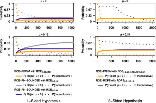
PRISM constrains the ROE to exclude the ROPE (Section 2). We assess operating characteristics when interval monitoring PRISM versus alternative ROE specifications. For a one-sided hypothesis, this includes comparing PRISM monitoring (ROE-PRISM) to a ROE that ranges from the point null to a minimally scientifically meaningful effect (ROE-PN-BOUNDED). For a two-sided hypothesis, we compare it to ROPE monitoring (ROE-ROPE).

Kruschke (2013) evaluated the limiting properties of ROE-ROPE monitoring using a 95% highest density interval for a two-armed randomized trial in which participants are randomized in blocks of size two and have standard normal outcomes under both arms. We replicated this setting and considered patients on the treatment arm to have outcomes drawn from $N({\mu }_T,1)$ with μ_T taking values of 0, 0.15, 0.325, and 0.50. Supposing a one-sided hypothesis, we set ROE-PRISM with ROE ${}_{(0.15,0.5)}$ and compared to two ROE-PN-BOUNDED designs specified by ROE ${}_{(0,0.5)}$ and ROE ${}_{(0,0.15)}$. In the two-sided hypothesis setting we set ROE-PRISM as with ROE ${}_{(-0.5,-0.15)\cup (0.15,0.5)}$ and compared to ROE-ROPE with a ROPE of [–0.15, 0.15]. For accumulating monitoring evaluations, we compared different ROE specifications regarding the probability of the SGPV to rule out the hypothesis $\mu \le 0$ (one-sided hypothesis) or μ = 0 (two-sided hypothesis) and of being SGPV inconclusive. We used unadjusted 95% confidence intervals for monitoring intervals starting with the fourth observation (i.e., monitoring frequencies: W = 4, S = 1, A = 0, and N = 5000). With a known variance, these intervals are mathematically equivalent to 6.83 support intervals and practically equivalent to 95% credible intervals with a flat prior on the mean.

From 20,000 Monte Carlo replicates, and under a one-sided hypothesis and treatment effect of 0, ROE-PRISM monitoring had a smaller limiting Type I error rate than monitoring either ROE-PN-BOUNDED hypothesis (Figure 3 and in supplemental material). Monitoring ROE-PN-BOUNDED with ROE ${}_{(0,0.5)}$ was slightly more quickly conclusive than ROE-PRISM monitoring. Under a two-sided hypothesis, the limiting SeqSGPV Type I error was nearly equivalent between ROE-PRISM and ROE-ROPE monitoring. Yet, ROE-PRISM monitoring was dramatically more quickly conclusive than ROPE monitoring which, at the ROPE boundary, had a risk of failing to be conclusive.

Fig. 3 Limiting probability of different ROE specifications for an interval to exclude μ = 0 (two-sided hypothesis) or $\mu \le 0$ (one-sided hypothesis) and of being PRISM inconclusive. In a one-sided hypothesis, setting the PRISM ROE to exclude practically equivalent or worse effects to the point null reduces Type I error. In a two-sided hypothesis, the PRISM closes monitoring for effects on ROPE boundaries compared to monitoring ROPE only. See Figure 2 for PRISM monitoring rules (also supplemental material) for limiting probabilities under other treatment effects.

In practice, many studies will not have the luxury of unrestricted monitoring or as large as 5000 observations. Under the same simulation setting, we impose a maximum sample size N ranging from W (the first monitoring evaluation) to 5000, and look at the Type I error trajectory across N for different monitoring frequencies (W, S, and A). We simulated 400,000 trials for each ROE monitoring scheme and a combination of W, S, and A. 100 different wait times were set to achieve an expected interval half-width of 0.05 to 0.75. To consider earlier wait times, an additional 10 wait times were set to achieve an expected interval width of from 0.75 to 1.96. S was set to 1 and 10 and A to 0 and 10. At each N from W to 5000, we estimated the proportion of trials making a Type I error at or before N.

Under these settings, monitoring the one-sided ROE-PRISM and ROE-PN-BOUNDED allowed for shorter minimum wait times than monitoring the two-sided ROE-PRISM and ROE-ROPE while controlling Type I error at 0.05 (Figure 4). Type I errors occurred more gradually under the one-sided ROE-PRISM than ROE-PN-BOUNDED. These results reemphasize the benefit of a ROPE in controlling Type I error and designing a trial that requires a smaller sample size. Increasing S and A better controlled Type I error across all designs and for both one- and two-sided hypotheses. Increasing to A = 10 had a bigger impact on controlling Type I error than increasing to S = 10 for all designs (see supplemental material). However, increasing S and A generally did not decrease the wait time required to control Type I error for most designs. Monitoring the one-sided ROE-PRISM was the exception. Increasing S and/or A allowed for shorter wait times while controlling Type I error. Monitoring frequencies worked synergistically with the one-sided PRISM to control Type I error. When monitoring the one-sided ROE-PRISM, the Type I error was less than 0.035 when S = 10 and A = 10 regardless of the maximum sample size and wait time.

Fig. 4 Type I error trajectory of different ROE specifications when SGPV interval monitoring given different monitoring frequencies W, S, A, and N. Given that μ = 0, an error occurs when, at a maximum sample size (N), an interval excludes the point null hypothesis. With an unadjusted 95% confidence interval, the first look W (denoted by circles) has an error rate of 0.05 for a two-sided hypothesis and 0.025 for a one-sided hypothesis. As accumulating data are evaluated at S and A, Type I error increases (trajectory following circle). Incorporating a ROPE can protect against Type I error. Except for ROE-PN-BOUNDED, the accumulating data can be large enough that interval estimation is entirely within ROPE (for the ROE-ROPE specification) or within ROME (for the ROE-PRISM specification) before stopping to exclude the point null. The non-monotone trajectory occurs because some intervals exclude the point null but are PRISM-inconclusive for the stopping rule at N; given a larger N, some of these intervals will stop without making a Type I error. Red trajectories are the earliest monitoring can begin while controlling Type I error at 0.05; orange trajectories have the smallest limiting Type I error. For scientific context, trajectories are overlayed upon the ROE specifications, and the x-axis includes the expected interval half-width (I-EHW).

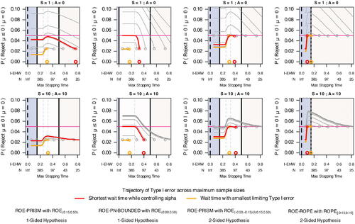
When monitoring ROE-PRISM and ROE-ROPE hypotheses, there was a point where Type I error decreased for increased maximum sample size. For PRISM monitoring, this point occurred when accumulated data had an expected interval half-width near the ROE midpoint. The decrease in Type I error occurred because, at a maximum sample size, a set of trials were PRISM- or ROPE-inconclusive despite their interval excluding the hypothesis of zero effect. These were counted as Type I errors for the maximum sample size. Yet, when followed until PRISM- or ROPE-conclusive, some of these trials no longer ended in a Type I error.

These simulations suggest that ROE-PRISM monitoring may have added Type I error benefits under delayed outcomes. Increasing S and/or A helps reduce the risk of reversing statistical significance when stopping a trial before delayed outcomes are observed (see supplementary material).

5 Interval versus Likelihood Ratio PRISM Monitoring

The goal of this work is to develop SeqSGPV for PRISM interval monitoring; however, we also consider monitoring PRISM using likelihood ratios. The likelihood ratio measures the evidence the data provides between two point-wise hypotheses. Wald (1945) developed the Sequential Probability Ratio Test to monitor accruing data until the likelihood ratio reaches a level of support for pre-specified hypotheses while controlling the false discovery rates. The symmetric Triangular Test by Anderson (1960) closes the sample size, which could be indefinite when the true parameter supports either hypothesis equally. In the supplementary material, we derive a symmetric, location-shifted Triangular Test used for one-sided PRISM monitoring, and we draw connections between likelihood ratios and likelihood support intervals. This section uses the location-shifted Triangular Test to compare and contrast PRISM monitoring using likelihood ratios (under the Triangular Test framework) versus likelihood support intervals. This comparison is not exhaustive in comparing the performance of different metrics in monitoring PRISM. However, it is a relevant starting point because likelihood ratios are foundational metrics to Bayes Factors and critical value hypothesis testing. These simulations highlight a key theme of this work of connecting stopping rules with the most plausible effects reflected by interval estimation.

Differences between SeqSGPV and the Triangular Test were investigated under the most simplistic setting: determining the effect of a single-arm study with independent observations drawn from $N(\mu ,1)$. A positive effect was considered beneficial, and a one-sided PRISM was supposed with ROE ${}_{(0.15,0.50)}$. Given the likelihood inferential framework of the Triangular Test, a 6.83 likelihood support interval is consistent with equal hypothesis error rates of 0.025. We compared three versions of the symmetric Triangular Test and a SeqSGPV design:

1. TT: Triangular Test comparing $H_1:\mu =0$ and $H_2:\mu ={\delta }_{G2}$, each with 0.025 error rates.

2. PRISM TT: Triangular Test comparing $H_1:\mu ={\delta }_{G1}$ and $H_2:\mu ={\delta }_{G2}$ with error rates for both of 0.025

3. PRISM TT T1E-Calibrated: Triangular Test comparing $H_1:\mu ={\delta }_{G1}$ and $H_2:\mu ={\delta }_{G2}$ with error rates equally calibrated so H₂ is supported at a rate of 0.025 when μ = 0.

4. PRISM SeqSGPV: Sequential SGPV monitoring of H_ROME and H_ROPE using 6.83 support intervals for monitoring with a 0.025 Type I error rate.

The Triangular Tests were fully sequential, beginning with the first observation. Fully sequential SeqSGPV began monitoring at the 12th observation to achieve the desired Type I error rate. We compared designs in their ability to draw consistent stopping rule conclusions with corresponding support intervals, their average sample size, and their probability of the SGPV rejecting the composite hypotheses: $\mu \le 0,\mu \in \mathit{\text{ROPE}},$ and $\mu \in \mathit{\text{ROME}}$. We drew estimates of these operating characteristics from 100K Monte Carlo simulations conditioning on μ ranging from–0.2 to 0.7.

Under μ = 0, the stopping rule conclusions were consistent with support intervals conclusions for TT, PRISM TT, and PRISM SeqSGPV (Figures 5). For TT and PRISM TT, the 6.83 support interval excluded H₂ when favoring H₁ (and vice-versa). By design, the PRISM SeqSGPV conclusion of ruling out ROPE or ROME was consistent with the 6.83 support interval excluding ROPE or ROME. In some SeqSGPV instances, ROME was ruled out while the 6.83 support interval excluded μ = 0. By prioritizing scientific relevance over statistical significance, the SeqSGPV PRISM conclusion is that scientifically meaningful effects are ruled out.

Fig. 5 SeqSGPV of a PRISM with ROE ${}_{(0.15,0.5)}$ is compared to three versions of the Triangular Test: TT compares μ = 0 to $\mu =0.5$ with 0.025 error rates; PRISM TT compares $\mu =0.15$ to $\mu =0.5$ with 0.025 error rates; and PRISM TT T1E-Calibrated compares $\mu =0.15$ to $\mu =0.5$ such that $\mu =0.5$ is favored at a rate of 0.025 when μ = 0. Top row: 6.83 support intervals at stopping under $\mu =0.325$ (ROE midpoint). 100K intervals are thinned to 200 intervals. Lighter shaded intervals in PRISM TT T1E-Calibrated do not exclude $\mu =0.5$ when $\mu =0.15$ is favored (and vice-versa). The rug in SeqSGPV are instances when an interval excludes zero-effect (i.e., statistically significant) and ROME. Bottom row: average sample size and error rates.

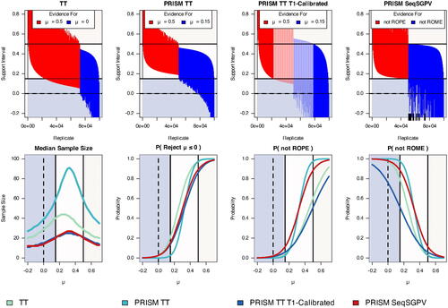
PRISM TT T1E-Calibrated conclusions were often consistent with support interval conclusions. When evidence favored H₂, μ = 0 was excluded from the support interval. However, the 6.83 support interval was sometimes inconsistent with stopping rule conclusions for $\mu =0.15$ and $\mu =0.5$. Some intervals included $\mu =0.15$ when the test provided evidence for $\mu =0.5$ (and vice-versa). This result is unsurprising because the design was calibrated to have a 0.025 error rate when μ = 0 yet allowed for error rates of 0.1385 for $\mu =0.15$ and 0.50. For consistent conclusions, the support interval’s boundaries for evidence should be set based on the error rates of the PRISM Triangular Test using 1.81 support intervals (mathematically equivalent to a 72% Confidence Interval). Alternatively, the error rates for H₁ and H₂ should be set to 0.025 as in PRISM TT.

Though not scientifically motivated, the Triangular Test induced a mathematical ROPE. When the TT design favored H₂, the support intervals had a lower bound no closer to 0 than 0.045. Still, this meant that when favoring H₂, some intervals provided evidence of effects practically equivalent to the point null (i.e., less than 0.15). PRISM TT T1E-Calibrated induced a stronger mathematical ROPE of 0.095 across all effects, though still less than 0.15. PRISM TT was the only Triangular Test considered to rule out ROPE when favoring H₂ and ROME when favoring H₁.

In contrast to TT, the remaining three PRISM-based designs had the desirable feature that ROME effects were supported 50% of the time at the ROE midpoint of 0.325 (Figure 5). The TT design favored H₂ in roughly 70% of the Monte Carlo replicates at the ROE midpoint. Closely related, the PRISM-based designs had the highest average sample size at the ROE midpoint, while TT had the largest average sample size at 0.25 (the midpoint of 0 and the ROME boundary).

PRISM SeqSGPV and PRISM TT T1E-Calibrated had essentially the same median sample size and were superior to TT and PRISM TT. At $\mu =0.25$, the average PRISM SeqSGPV sample size was half that of TT, and at $\mu =0.325$, the PRISM SeqSGPV average sample size was still lower than TT. In a tradeoff, TT and PRISM TT were more strongly powered for the 6.83 support interval to exclude $\mu \le 0$. PRISM SeqSGPV was more likely to rule out ROPE than TT and PRISM TT T1E-Calibrated. This was desirable for ROE and ROME effects, though undesirable for ROPE effects. Similarly, PRISM SeqSGPV had a higher probability of ruling out ROME effects which was desirable for ROE and ROPE effects but undesirable for ROME effects.

In summary, the Triangular Test has similarities to SeqSGPV by closing the monitoring sample size and comparing two pre-specified scientifically meaningful hypotheses. Both stopping rules are best aided by an end-of-study interval to estimate the most plausible values of the effect. In these simulations, the average sample size was largest at the midpoint between the two hypotheses under evaluation. Both sequential monitoring schemes induced a ROPE. The Triangular Test ROPE was mathematically induced and did not align with a scientifically meaningful ROPE. To mimic SeqSGPV monitoring, in which a 6.83 interval rules out ROPE or ROME effects, the PRISM Triangular Test required a large sample size for 0.025 error rates or a relaxation of error rates coupled with a less informative support interval. Differences in interpreting likelihood ratios versus SGPVs are highlighted in Section 3.3 and the supplemental material.

6 Applying SeqSGPV to the REACH Trial

The Rapid Education/Encouragement And Communications for Health (REACH) randomized clinical trial (Nelson et al. 2018; Mayberry et al. 2019, 2020; Nelson et al. 2021) was designed to help adults with type 2 diabetes improve glycemic control (as measured by HbA1c; for simplicity, we hereafter omit the unit of measurement which is %) and adhere to medication. Participants were randomized into one of three treatment arms with a 2:1:1 allocation ratio: enhanced treatment as usual (a text message when study HbA1c results are available), frequent diabetes self-care support text messages, and frequent diabetes self-care support text messages with monthly phone coaching. A meaningful, equally allocated two-group comparison in this study was enhanced treatment as usual versus frequent self-care support. Follow-up assessments occurred at 3, 6, 12, and 15 months with 12-month HbA1c as the primary outcome. The study recruited about six participants a week and 300 a year.

The median REACH baseline HbA1c was 8.20 [IQR of 7.20, 9.53], and in this population, lower HbA1c reflects improved glycemic control. A change from baseline HbA1c of no more than ± of 0.15 is considered practically equivalent to no change. In contrast, a decrease of HbA1c of 0.5 is scientifically meaningful to the point of adopting this novel intervention. The study was designed to test a two-sided hypothesis through significance testing and to report estimated confidence intervals. However, this approach does not directly connect to the pre-specified scientific interpretation. For these purposes, we simulate how this trial could have been conducted with monitoring a pre-specified PRISM using the SGPV, via SeqSGPV.

We simulated the operating characteristics of adaptively monitoring the REACH trial using SeqSGPV PRISM monitoring. For demonstration, we assumed instantaneous outcomes using a two-sided PRISM with ROE ${}_{(-0.50,-0.15)\cup (0.15,0.50)}$ and a one-sided PRISM with ROE ${}_{(-0.50,-0.15)}$ for N of 512, 650, and unrestricted. Then, to mimic real-life, we simulated a trial using a one-sided PRISM with 300 delayed outcomes for the same maximum sample sizes. To determine the minimum wait time, we suppose the trial would want an end-of-study interval width to be no more than 1.5 (the outcome standard deviation is 2), which means setting W to no less than 55 observations while achieving desired Type I error control.

The two-sided PRISM was monitored with frequencies W = 420, S = 25, A = 0, and N = 512, and the one-sided PRISM was monitored with frequencies W = 55, S = 25, A = 0, and N = 512. An ordinary least square regression model was fit on accumulating data, and SeqSGPV monitored unadjusted 95% confidence intervals to estimate the treatment effect. To reduce Type I error, we also monitored the one-sided PRISM with frequency W = 55, S = 25, and A = 25.

For treatment effects ranging from–1 to 1 by 0.025, we generated 120,000 bootstrap samples from REACH twelve-month HbA1c outcomes. In simulating the trial, participants were randomized in block two fashion to usual versus frequent self-care support. Outcomes followed the potential outcomes framework where Y(0) equaled the 12-month outcome if randomized to the control arm and Y(1) equaled Y(0) plus the treatment effect if randomized to treatment.

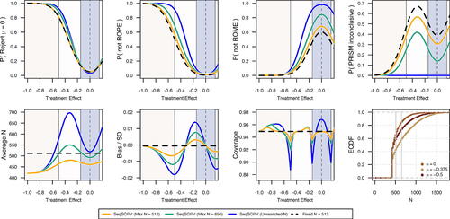
Under the two-sided PRISM and supposing immediate outcomes, the average sample size ranged from 421 to 480 under the constraint of $N=$512 (Figure 6). This was sufficient for the study to be 81% powered to reject $\mu \le 0$ for a treatment effect of–0.5 with a Type I error of 0.05. These error rates were equivalent to a single assessment at N = 512. The chance of stopping earlier under treatment effects of 0 and–0.5 were, respectively, 0.66 and 0.59. The average sample size was largest at the ROE midpoint of–0.325. Bias, defined as the expected value of the difference between the estimate and true effect, was no worse than an absolute standardized effect size of 0.02. There was no bias at the midpoint of ROE, and bias pulled toward the null for effects closer to the null and vice-versa. Compared to a single assessment at N = 512, the PRISM design was less likely to be PRISM inconclusive and more likely to find non-ROPE effects as non-ROPE and non-ROME effects as non-ROME.

Fig. 6 Operating characteristics from monitoring a two-sided PRISM on assumed immediate REACH trial outcomes.

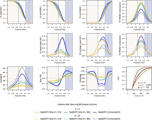
Supposing immediate outcomes with a one-sided PRISM, the average sample size ranged from 115 to 325 under the constraint of N = 512 and A = 0 (see supplemental material). This was sufficient to power the study as the two-sided PRISM with equivalent Type I error. Undercoverage was most extreme at the ROWPE and ROME boundaries and bias was as much as 0.1 of an absolute standardized effect size. Requiring A = 25 increased the average sample size yet reduced Type I error and bias. For unrestricted sample sizes, A = 25 increased the probability of finding non-ROPE effects as non-ROPE and non-ROME effects as non-ROME. However, under maximum sample sizes, A = 25 increased the probability of ending PRISM inconclusive.

In a real-life setting of 300 delayed outcomes, the average sample size for monitoring the one-sided PRISM ranged from 408 to 476 for A = 0 and 437 to 495 for A = 25 (Figure 7). Due in part to fewer monitoring opportunities, the Type I error was 0.025 for A = 0 and A = 25 and power was 0.78 for a treatment effect of–0.5. The chance of stopping early under a treatment effect of 0 was 0.58 (A = 0) and 0.44 (A = 25). The affirmation step of A = 25 decreased the risk of Type I error reversals from 0.03 (A = 0) to 0.01. For nonzero effects, the chance of newly rejecting H₀ was less under A = 25 than A = 0 when under a maximum sample size of 512 and 650. With an unrestricted sample size, the chance of newly rejecting H₀ for a treatment effect at the ROE mid-point was 0.08 for both A = 25 and A = 0. The following are possible end-of-study SGPV conclusions.

Fig. 7 Operating characteristics from monitoring a one-sided PRISM on data from the REACH trial in which outcomes were delayed by 300 observations.

1. The estimated mean difference was–0.51 (95% confidence interval:–0.86,–0.16) which is evidence that the treatment effect is at least practically better than the point null hypothesis (p_ROWPE = 0) with some evidence for being scientifically meaningful (p_ROME = 0.52).

2. The estimated mean difference was 0.03 (95% confidence interval:–0.49, 0.55) which is evidence that the treatment effect is not scientifically meaningful (p_ROME = 0) with some evidence for being practically equivalent or worse than the point null is (p_ROWPE =0.67).

3. The estimated mean difference was–0.29 (95% confidence interval:–0.56,–0.02) at the maximum sample size, which is inconclusive evidence to rule out practically equivalent or worse effect than the point null (p_ROWPE = 0.24) and scientifically meaningful effects (p ${}_{\mathit{\text{ROME}}}=0.11$). There is more evidence that the effect is practically equivalent or worse than the point null than scientifically meaningful.

Note that the third example prioritizes scientific relevance over statistical significance. For each conclusion, the following clarification may be provided for a design (in this case for N = 650 and A = 25): Based on simulations, there may be an absolute bias, in terms of effect size, as large as 0.01 of a standard deviation and interval coverage as low as 0.94.

7 Discussion, Limitations, and Extensions

SeqSGPV is a novel monitoring scheme tailored to SGPV inference. It connects trial design intentions, such as powering to detect a minimally scientifically meaningful effect, with end-of-study inference. In the context of interval monitoring of superiority studies, the PRISM closes the sample size which could continue indefinitely when only monitoring ROPE while still benefiting from reducing the Type I error. SeqSGPV prioritizes drawing conclusions on scientific relevance over statistical significance.

While this work lays out a general framework for SeqSGPV, it neither requires nor addresses how to estimate effects and intervals without bias and with correct coverage. This limitation can be reduced with fewer stopping rule evaluations and/or an increased affirmation step. “Repeated Confidence Intervals” is a strategy to correct coverage; and, an extension could be to monitor with bias-corrected intervals that account for PRISM monitoring. Because “Repeated Confidence Intervals” are based on group sequential methods and recursive calculations of error rates, study designs could be determined analytically with a reliance upon asymptotic theory as needed.

While the affirmation step has been used in dose-finding studies, we highlight it here in a broader context. In these simulations, it provides a means for reducing false discoveries and the risk of reversing conclusions under delayed outcomes. Further extensions to SeqSGPV could incorporate stopping rules that condition upon unobserved data, such as posterior probabilities of success and conditional power.

As with any monitoring scheme, it is imperative to evaluate the frequency properties under model misspecification. We suggest simulating departures from the model which is doable through the R package SeqSGPV.

Supplemental Materials

The supplemental material includes visual examples of SeqSGPV PRISM monitoring with an affirmation step; an overview of minimal assumptions and conclusions drawn from alternative sequential monitoring metrics; details on modifying the symmetric Triangular Test for PRISM monitoring; the beneficial impact of look frequency and an affirmation step when observing delayed outcomes; and additional figures expanding upon the simulation settings presented as main results.

Acknowledgments

The authors also thank the helpful feedback and reviews by the editor, associate editor, and reviewers.

Disclosure Statement

The authors report there are no competing interests to declare.

Additional information

Funding

This work was supported by the Center for High Performance Computing at the University of Utah, the Advanced Computing Center for Research and Education at Vanderbilt University, and the grant NIDDK R01 DK100694.

References

- Anderson, T. W. (1960), “A Modification of the Sequential Probability Ratio Test to Reduce the Sample Size,” The Annals of Mathematical Statistics, 101, 102505. DOI: 10.1214/aoms/1177705996.
- Birnbaum, A. (1962), “On the Foundations of Statistical Inference,” Journal of the American Statistical Association, 57, 269–306. DOI: 10.1080/01621459.1962.10480660.
- Blume, J. D., DAgostino McGowan, L., Dupont, W. D., and Greevy Jr., R. A. (2018), “Second-Generation P-Values: Improved Rigor, Reproducibility, & Transparency in Statistical Analyses,” PloS One, 13, e0188299. DOI: 10.1371/journal.pone.0188299.
- Blume, J. D., Greevy, R. A., Welty, V. F., Smith, J. R., and Dupont, W. D. (2019), “An Introduction to Second-Generation p-Values,” The American Statistician, 73, 157–167. DOI: 10.1080/00031305.2018.1537893.
- Freedman, L. S., Lowe, D., and Macaskill, P. (1984), “Stopping Rules for Clinical Trials Incorporating Clinical Opinion,” Biometrics, 40, 575–586.
- Goodman, S. N., Zahurak, M. L., and Piantadosi, S. (1995), “Some Practical Improvements in the Continual Reassessment Method for Phase I Studies,” Statistics in Medicine, 14, 1149–1161. DOI: 10.1002/sim.4780141102.
- Hobbs, B. P., and Carlin, B. P. (2008), “Practical Bayesian Design and Analysis for Drug and Device Clinical Trials,” Journal of Biopharmaceutical Statistics, 18, 54–80. DOI: 10.1080/10543400701668266.
- Jennison, C., and Turnbull, B. W. (1989), “Interim Analyses: The Repeated Confidence Interval Approach,” Journal of the Royal Statistical Society, Series B, 51, 305–334. DOI: 10.1111/j.2517-6161.1989.tb01433.x.
- Korn, E. L., Midthune, D., Chen, T. T., Rubinstein, L. V., Christian, M. C., and Simon, R. M. (1994), “A Comparison of Two Phase I Trial Designs,” Statistics in Medicine, 13, 1799–1806. DOI: 10.1002/sim.4780131802.
- Kruschke, J. K. (2011), “Bayesian Assessment of Null Values via Parameter Estimation and Model Comparison,” Perspectives on Psychological Science, 6, 299–312. DOI: 10.1177/1745691611406925.
- ——(2013), “Bayesian Estimation Supersedes the t test,” Journal of Experimental Psychology. General, 142, 573–603.
- ——(2018), “Rejecting or Accepting Parameter Values in Bayesian Estimation,” Advances in Methods and Practices in Psychological Science, 1, 270–280. DOI: 10.1177/2515245918771304.
- Mayberry, L. S., Berg, C. A., Greevy, R. A., Nelson, L. A., Bergner, E. M., Wallston, K. A., Harper, K. J., and Elasy, T. A. (2020), “Mixed-Methods Randomized Evaluation of FAMS: A Mobile Phone-Delivered Intervention to Improve Family/Friend Involvement in Adults’ Type 2 Diabetes Self-Care,” Annals of Behavioral Medicine, 55, 165–178. DOI: 10.1093/abm/kaaa041.
- Mayberry, L. S., Bergner, E. M., Harper, K. J., Laing, S., and Berg, C. A. (2019), “Text Messaging to Engage Friends/Family in Diabetes Self-Management Support: Acceptability and Potential to Address Disparities,” Journal of the American Medical Informatics Association, 26, 1099–1108. DOI: 10.1093/jamia/ocz091.
- Nelson, L. A., Greevy, R. A., Spieker, A., Wallston, K. A., Elasy, T. A., Kripalani, S., Gentry, C., Bergner, E. M., LeStourgeon, L. M., Williamson, S. E., and Mayberry, L. S. (2021), “Effects of a Tailored Text Messaging Intervention Among Diverse Adults With Type 2 Diabetes: Evidence From the 15-Month REACH Randomized Controlled Trial,” Diabetes Care, 44, 26–34. DOI: 10.2337/dc20-0961.
- Nelson, L. A., Wallston, K. A., Kripalani, S., Greevy Jr., R. A., Elasy, T. A., Bergner, E. M., Gentry, C. K., and Mayberry, L. S. (2018), “Mobile Phone Support for Diabetes Self-Care Among Diverse Adults: Protocol for a Three-Arm Randomized Controlled Trial,” JMIR Research Protocols, 7, e92. DOI: 10.2196/resprot.9443.
- Royall, R. (1997), Statistical Evidence: A Likelihood Paradigm (Vol. 71), Boca Raton, FL: CRC Press.
- Sirohi, D., Chipman, J., Barry, M., Albertson, D., Mahlow, J., Liu, T., Raps, E., Haaland, B., Sayegh, N., Li, H., Rathi, N., Sharma, P., Agarwal, N., and Knudsen, B. (2022), “Histologic Growth Patterns in Clear Cell Renal Cell Carcinoma Stratify Patients into Survival Risk Groups,” Clinical Genitourinary Cancer, 20, e233–e243. DOI: 10.1016/j.clgc.2022.01.005.
- Stewart, T. G., and Blume, J. (2019), “Second-Generation p-values, Shrinkage, and Regularized Models,” Frontiers in Ecology and Evolution, 7, 486. DOI: 10.3389/fevo.2019.00486.
- US Food and Drug Administration. (2010), Guidance for the Use of Bayesian Statistics in Medical Device Clinical Trials, Maryland: US Food and Drug Administration.
- Wald, A. (1945), “Sequential Tests of Statistical Hypotheses,” The Annals of Mathematical Statistics, 16, 117–186. DOI: 10.1214/aoms/1177731118.
- Zuo, Y., Stewart, T. G., and Blume, J. D. (2021), “Variable Selection With Second-Generation P-Values,” American Statistician, 76, 91–101. DOI: 10.1080/00031305.2021.1946150.