High-dimensional propensity score and its machine learning extensions in residual confounding control

Abstract

“The use of health care claims datasets often encounters criticism due to the pervasive issues of omitted variables and inaccuracies or mis-measurements in available confounders. Ultimately, the treatment effects estimated utilizing such data sources may be subject to residual confounding. Digital electronic administrative records routinely collect a large volume of health-related information; and many of which are usually not considered in conventional pharmacoepidemiological studies. A high-dimensional propensity score (hdPS) algorithm was proposed that utilizes such information as surrogates or proxies for mismeasured and unobserved confounders in an effort to reduce residual confounding bias. Since then, many machine learning and semi-parametric extensions of this algorithm have been proposed to better exploit the wealth of high-dimensional proxy information. In this tutorial, we will (i) demonstrate logic, steps and implementation guidelines of hdPS utilizing an open data source as an example (using reproducible R codes), (ii) familiarize readers with the key difference between propensity score vs. hdPS, as well as the requisite sensitivity analyses, (iii) explain the rationale for using the machine learning and double robust extensions of hdPS, and (iv) discuss advantages, controversies, and hdPS reporting guidelines while writing a manuscript.”

KEYWORDS:

• high-dimensional propensity score
• machine learning
• double robust
• electronic administrative records
• proxy

Disclaimer

As a service to authors and researchers we are providing this version of an accepted manuscript (AM). Copyediting, typesetting, and review of the resulting proofs will be undertaken on this manuscript before final publication of the Version of Record (VoR). During production and pre-press, errors may be discovered which could affect the content, and all legal disclaimers that apply to the journal relate to these versions also.

1 Introduction

Originally developed to address residual confounding in observational health administrative and claims data sources, the High-dimensional Propensity Score (hdPS) algorithm has proven its efficacy and versatility across various domains (Schneeweiss et al. 2009). Since its inception in 2009, the hdPS algorithm has been widely utilized in demonstrating the effectiveness of medical products and in conducting health services and utilization research (see Appendix Table 1 and Appendix Figure 1) (Schneeweiss 2018). Over time, the hdPS algorithm has been applied in the context of time-dependent confounding (Neugebauer et al. 2015) and unstructured free-text health information (Afzal et al. 2019). In terms of methodological advancements, in recent years, the hdPS algorithm has embraced the integration of machine learning techniques and double robust estimators, enhancing its ability to extract from big data sources and improving its statistical properties (Wyss et al. 2022; Ju et al. 2019b).

While methodologists have shown great enthusiasm for the algorithm and its extensions (Ju, Benkeser, and van Der Laan 2020; Cheng et al. 2020; Ju et al. 2019a; Wyss et al. 2018b; Shortreed and Ertefaie 2017), practitioners often encounter challenges in understanding the underlying rationale and in implementing the algorithm effectively in their own research endeavors. To bridge this gap, the objective of this tutorial is to provide a comprehensive and accessible guide to the hdPS approach. We will thoroughly explain the rationale, step-by-step procedures, and details involved in implementing the hdPS algorithm. By doing so, we aim to empower practitioners with a clear understanding of when and how to apply the hdPS approach appropriately in their specific research contexts.

To ensure the tutorial’s applicability and reproducibility, we will use the publicly available National Health and Nutrition Examination Survey (NHANES) data (for Disease Control and Prevention 2021). This dataset, being widely accessible, ensures readers can procure the necessary data. Additionally, we will illustrate the process using openly accessible R packages (Robert 2020; Greifer 2022; Zeileis, Köll, and Graham 2020; Friedman, Hastie, and Tibshirani 2010; Gruber and van der Laan 2012; Polley et al. 2023). The software codes embedded in this article, along with the linked Github repository (Karim 2023a), allow for easy replication of the methods discussed. By engaging with this tutorial, readers will be equipped with tools and resources for integrating the hdPS algorithm into their research projects.

2 Motivating example

We are going to be discussing diabetes, a metabolic condition characterized by elevated blood sugar levels and an inability to effectively utilize insulin, commonly known as insulin resistance. Various studies suggest that obesity plays a significant role in increasing the risk of diabetes (Klein et al. 2022). The potential explanation is that excess body fat may induce insulin resistance (Hardy, Czech, and Corvera 2012), thereby hampering the body’s capacity to maintain normal blood sugar levels.

Our focal point of research in this tutorial is, “Does obesity elevate the risk of diabetes development?” While the primary purpose of this tutorial is not to solve a clinical question or draw definitive conclusions about the connection between obesity and diabetes in the general populace, it does serve as an engaging scenario for illustrating how to deploy the hdPS algorithm by leveraging publicly available data.

Hypothesized Causal Diagram and Data Source

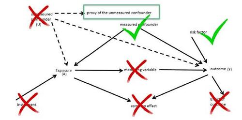
We have utilized a causal diagram (Greenland, Pearl, and Robins 1999) based on our comprehensive review of the literature (Figure 1) (Saydah et al. 2014; Liu et al. 2013; Kabadi, Lee, and Liu 2012; Ostchega et al. 2012). To address our research question, we have relied on the NHANES data, which can be obtained freely from the US Centers for Disease Control (CDC) and Prevention website (for Disease Control and Prevention 2021). We have specifically examined the available variables from three NHANES data cycles: 2013-2014, 2015-2016, and 2017-2018. A detailed overview of these variables is provided in Table 1. Due to the lengthy and often restricted process of acquiring claims databases, we opted to utilize publicly available survey data in order to ensure reproducibility of the results. The software codes can be accessed in the author’s GitHub repository (Karim 2023a).

Unmeasured confounding

Unfortunately, when working with secondary data sources such as NHANES, researchers do not have control over which variables are included in the survey. The same issue also occurs in the health administrative data settings, where the data is primarily collected for non-research (e.g., administrative and billing) purposes. Consequently, it is possible that some essential variables needed to address specific research questions may be unavailable. In our specific causal diagram, one of the known confounding factors for the association of interest is the burden of comorbidities or pre-existing medical conditions (Kong et al. 2013). Individuals with a greater overall burden of disease might be more likely to be obese due to various factors such as reduced physical activity, altered metabolic status, or the use of certain medications (Malone 2005). Simultaneously, those with a higher burden of comorbid conditions might be at an increased risk for developing diabetes due to the cumulative stress and metabolic impact of their multiple health conditions, irrespective of their obesity status (Longarela et al. 2000). Thus, a higher level of comorbidity might independently be associated with both obesity and diabetes.

Researchers often employ various comorbidity scores, such as the Charlson Comorbidity Index, Elixhauser Comorbidity Index, or Chronic Disease Score (Charlson et al. 1987; Elixhauser et al. 1998; Von Korff, Wagner, and Saunders 1992; Austin et al. 2015), to quantify this concept. Unfortunately, in the case of NHANES, the collection of certain disease-specific information necessary for calculating these comorbidity scores is lacking. The inability to account for such a confounding factor may introduce bias and residual confounding in the estimation of treatment effects (Schneeweiss and Maclure 2000; Lix et al. 2011, 2013).

Proxy Adjustment

In the epidemiological studies, a number of empirical criteria that are proposed to identify adjustment variables. Theses criteria are most useful in practical settings where causal diagrams are hard to draw, or when some variables in the minimum adjustment sets are unavailable. Modified disjunctive cause criterion, a popular approach, advocates to adjust for variables that are (a) causes of exposure or outcome or both, (b) discard known instrument(s), and (c) including good proxies for unmeasured common causes (VanderWeele 2019). Using this principle, in our present analysis, we could try to identify other variables that are good proxies of comorbidity burden.

Fortunately, within the NHANES survey, the Prescription Medications (RXQ_RX) component is available, which captures data on prescription medications taken within the past 30 days of the survey. These surveys are administered by trained interviewers, and efforts are made to ensure data cleanliness through quality control procedures. The International Classification of Diseases, 10th Revision, Clinical Modification (ICD-10-CM) is a standardized coding system used to classify diseases, disorders, and injuries (Hirsch et al. 2016). In the NHANES survey, the interviewers categorize and convert the collected information on prescription medications into ICD-10 codes.

It is worth noting that the ICD-10-CM system captures a wide range of prescriptions that are indicative of certain disease conditions (see Table 2 for a sample). Within the context of our specific research question, it remains unclear what role these prescriptions and conditions play, and how to appropriately summarize this vast amount of additional information for our data analysis. ‘Count of prescriptions’ is often used to measure comorbidity burden (Farley, Harley, and Devine 2006). This is not a perfect measure, but could serve as a crude proxy for our purpose according to the modified disjunctive cause criterion.

3 Key idea of High-dimensional Propensity score

Although many ICD-10-CM codes for various prescription medications may not be directly interpretable within the context of the research question (i.e., obesity elevating the risk of diabetes), they can still offer valuable insights into the overall health status of the patients from whom they are collected (Schneeweiss 2018). As a result, these codes could collectively serve as proxies, supplementing unmeasured information and contributing to our understanding of the research context.

Similarly, within broader health administrative data source contexts, diverse classifications are used to code diagnoses (e.g., ICD-9), procedures (e.g., Current Procedural Terminology: CPT), medications (e.g., National Drug Code: NDC, Anatomical Therapeutic Chemical classification: ATC), and other aspects (e.g., Primary Care Physician visits: PCP). As a result, these datasets may contain a plethora of additional codes related to patients. The challenge involves determining which codes are relevant for our analysis and which may introduce unnecessary noise.

To address this challenge, Schneeweiss and colleagues proposed a multi-step algorithm for effectively leveraging these codes in our analysis (Schneeweiss et al. 2009). The core idea involves empirically identifying and utilizing proxies that may provide valuable information related to unobserved or imprecisely observed confounders. Although it may not be feasible to directly measure the correlation between an unmeasured confounder (e.g., comorbidity burden in our example) and a measured proxy variable or code (e.g., simple count of existing prescriptions), we can explore the relationship between a measured proxy variable and the outcome variable while adjusting for the exposure variable. By doing so, we can assess whether the inclusion of proxy information has an impact on the crude association between the outcome and the exposure. This approach enables us to evaluate the potential relevance of various proxies and rank them based on their influence on the crude association, for us to be able to select an useful subset of proxies. This concept forms the fundamental basis of the hdPS algorithm.

The hdPS algorithm’s key implication is that using informative proxies collectively and eliminating irrelevant codes can lead to a more effective adjustment strategy than merely adjusting for one proxy of an unmeasured confounder (e.g., ‘Count of prescriptions’ variable, as previously outlined in our example). In the subsequent discussion, we will thoroughly explore each of the steps delineated in the original hdPS algorithm. This will provide a comprehensive overview of the sequential procedures involved in implementing the algorithm, allowing for a deeper understanding of its complexities and potential benefits. See Table 3 for an overview of these steps.

Step 0: Creating analytic data based on eligibility criteria

Identify key variables: This initial step serves as a preparatory stage prior to conducting the hdPS analysis. It involves the creation of an analytic dataset, similar to conventional epidemiological studies, that includes variables with clearly defined roles based on the causal diagram (or a suitable empirical criterion) of the research question are included. These variables typically encompass the outcome, exposure, confounders, and risk factors associated with the outcomes of interest.

Merge data: To carry out this step, we accessed data from three cycles of the NHANES dataset, which were obtained from the US CDC website. These datasets underwent a standardization process to ensure consistency across cycles. Specifically, we included the same variables mentioned in Table 1 for each cycle, and each variable was coded uniformly across all cycles. By merging the data from the three cycles, we created a unified and comprehensive analytic dataset.

Eligibility criteria: To facilitate the explanation of the hdPS algorithm, we narrowed our focus to a specific study population based on eligibility criteria. We defined eligible individuals as those who met the following criteria: a) aged 20 years or older and b) not pregnant during the data collection period. This exclusion of pregnant individuals is due in part to the transient nature of gestational diabetes, which typically resolves post-pregnancy and is driven by unique physiological mechanisms (McIntyre et al. 2019). For this tutorial, we have adopted a streamlined approach, considering only complete case data and requiring participants to have available ICD-10-CM codes, thereby ensuring the availability of sufficient proxy information for subsequent analysis, as discussed in the next step. This strategic choice highlights the explanation of the hdPS algorithm and its implementation, allowing us to present it in a clear and concise manner. Consequently, it avoids the need to engage with additional complexities and analytic steps needed to mitigate issues arising from missing or sparse data for investigator-specified and proxy covariates, respectively.

Step 1: Identification of proxy data sources (dimensions)

The first step of this algorithm is to identify additional data sources (or dimensions) linked to the analytical data, from which proxy variables will be created. For example, in a previous study based on data from the United Kingdom’s Clinical Practice Research Datalink, authors used p = 4 data sources or dimensions: (a) general practice data, (b) diagnosis data, (c) procedure data, and (d) medication data (Karim, Pang, and Platt 2018) (see Figure 2).

In the context of our tutorial, NHANES includes a component in the Sample Person Questionnaire that focuses on dietary supplements and prescription medications. Specifically, the questionnaire dedicated to prescription medication (RXQ_RX) gathers data regarding the usage of such drugs in the past 30 days leading up to the interview date of the participant. In our tutorial, we only include this prescription domain of ICD-10-CM codes. Hence the number of data source or dimension, p = 1 in this exercise. In selection of the ICD-10-CM codes, we need to consider two points:

1. Covariate assessment window (CAW): Analysts selectively collect proxy information within a CAW to establish the temporal window from which the ICD-10-CM codes will be obtained. It is crucial to ensure that this proxy information is collected prior to the commencement of the study or before measuring the exposure variable (Connolly et al. 2019; Schneeweiss et al. 2009), as illustrated in Figure 3. Intentionally collection of proxy information from a pre-exposure window aims to minimize the possibility of incorporating mediators or colliders in the subsequent analyses. During the NHANES interview conducted at the mobile examination center, information on body measures, which serve as the exposure status in our study, was collected. In our specific case, the CAW was defined as the 30-day window preceding the interview. Typically, in longitudinal claims databases, a 6-month CAW is considered, although durations of 1-2 years or more are also feasible (Thurin et al. 2022; Tazare et al. 2020). A longer CAW allows for the integration of more proxy information. However, depending on the study context, shorter CAW is also possible (e.g., 90 days prior to pregnancy start) (Suarez et al. 2023).

2. Omit duplicated information: We need to remove ICD-10-CM codes that could be close proxies of exposure and/or outcome (see Table 4), or other investigator-specified covariates we have already selected in step 0 to avoid any duplication. In general, excluding related codes or close proxies for investigator-specified covariates from the hdPS algorithm is crucial to avoid the risk of double-adjusting for variables or concepts already included in the final model (Judkins et al. 2007). While an automated process aids in proxy selection in later stages, a comprehensive understanding of the dataset by the analyst team is vital for the early identification and manual removal of problematic variables (Rassen et al. 2023b). This involves using clinical judgment to manually exclude codes, particularly those that are duplicates or closely related to investigator-specified variables (Schneeweiss et al. 2009). Additionally, the team must be vigilant against other potentially problematic variables, such as near-instrument variables (those predicting exposure but unrelated to the outcome) and colliders (a common effect of multiple variables), consistent with practices in previous hdPS studies (Brookhart, Rassen, and Schneeweiss 2010; Myers et al. 2011; Patrick et al. 2011). For studies spanning the transition from ICD-9 to ICD-10, utilizing mapping tables to align codes across these versions for the same data dimension is essential. R Code chunk 1 (see Appendix R code chunks) illustrates the exclusion of specific ICD-10-CM codes associated with the exposure and outcome from further analysis.

Other than these points, the proximity of the proxy information relative to exposure (temporally) has been considered in a few hdPS applications (Rassen et al. 2023b; Schneeweiss 2018). However, given CAW is short in our example, we did not consider this point.

Table 5 shows an example of 3 digit codes for 1 patient with subject ID “100001” following the exclusion of duplicate information related to exposure and outcome. We create the same for all patients. We merge all such proxy information with the analytic data created in step 0. After applying the eligibility criteria, we ended up with 7, 585 patients (see Appendix Figure 2).

Step 2: Identify the candidate empirical covariates based on prevalence

The granularity of the ICD-10-CM code, referring to the level of specificity or detail provided by the number of digits in the code, is a crucial decision that must be determined. For instance, codes with more digits (e.g., E11.4: Type 2 diabetes mellitus with neurological complications) generally indicate a more specific diagnosis, whereas codes with fewer digits offer a broader categorization of a condition (e.g., E11: Type 2 diabetes mellitus). In our case, we have chosen 3-digit codes to define the level of specificity in detailing medical diagnoses, striking a balance between generalized categorization and detailed diagnostic information.

Table 6 provides the frequency of the ICD-10-CM codes, truncated to three digits, in our dataset during the covariate assessment window. Some codes may exhibit lower counts, such as those below 20 or 10. Dealing with low counts or rare events in data modeling can substantially impact the precision and reliability of statistical estimates, potentially yielding results that do not accurately mirror the underlying population. This issue becomes especially problematic in scenarios where statistical models or machine learning algorithms are applied, as the model might overfit to these infrequent occurrences or generate unreliable predictions (Ogundimu 2019).

The main objective of this step is to identify and eliminate these less frequent codes to prevent numerical instability during our analysis. To achieve this, we can consider one of the following strategies:

1. Analysts can order the codes by prevalence (from high to low), and then select the top n ICD-10-CM codes with the highest prevalence. In the original algorithm, n was suggested to be 200 (Schneeweiss et al. 2009). However, there has been concern that this restriction might exclude some useful proxies (Schuster, Pang, and Platt 2015). A factor’s lower prevalence does not necessarily imply that it cannot influence or confound a relationship.

2. Another approach is to discard the codes with zero variance, i.e., codes that are either present for everyone or absent for everyone (Franklin et al. 2015; Karim, Pang, and Platt 2018). Although this methods effectively avoids multicolinearity, this method might still retain some low-prevalence codes (e.g., that are very close to zero).

3. Finally, analysts could specify a minimum number of patients, for example, 20, that must have a particular code for it to be included in the list (Robert 2020). This method likely provides a balanced compromise between the first two strategies.

By adopting the third approach, we have identified a total of n = 126 codes that meet the criteria for inclusion as ‘candidate empirical covariates.’ These covariates are referred to as ‘candidate empirical covariates’ because the algorithm will employ a proxy selection strategy on them later. Not all proxy variables created at this stage will necessarily be included in the final analysis. R Code chunk 2 (see Appendix R code chunks) demonstrates how to implement this step in R.

It is important to note that when working with multiple data dimensions, we need to calculate the empirical covariates separately for each data source or dimension. The decision regarding the granularity of the codes does not necessarily have to be the same across all data dimensions.

Step 3: Generate recurrence covariates based on frequency

In this step, we determine the frequency of occurrence of each ICD-10-CM code for each patient during the covariate assessment window (Schneeweiss et al. 2009). For each candidate empirical covariate identified in the previous step, we generate three binary recurrence covariates (R) based on the following criteria: (1) occurred at least once, (2) occurred sporadically (at least more than the median), and (3) occurred frequently (at least more than the 75th percentile). Table 7 provides examples of the three binary recurrence covariates created for each candidate empirical covariate from step 2, illustrating the process. The Bross formula used in Step 4 (see below) requires all variables of interest (exposure, outcome, and recurrence covariates) to be binary. To satisfy this requirement, we have transformed the empirical covariates into binary recurrence variables in the current step. R Code chunk 3 (see Appendix R code chunks) shows how to implement this step.

Given that we had one source or dimension of proxy data, denoted as p = 1, and we identified 126 candidate empirical covariates in step 2 (with the minimum number of patients in each code set to 20), we theoretically could have had a maximum of $p\times n\times 3$ binary recurrence covariates, which equals $1\times 126\times 3=378$. In the original hdPS algorithm, all possible binary recurrence covariates were stored and used in the next step (step 4) (Schneeweiss et al. 2009). However, later implementations considered a reduced number of recurrence covariates. In these implementations, if two or all three recurrence covariates are identical, only one distinct recurrence covariate is considered (Robert 2020). In our tutorial, we have adopted this latter strategy. For example, if most patients in our dataset experienced at least one episode of the common cold during the covariate assessment window, the ICD-10-CM code ‘J00 Acute nasopharyngitis [common cold]’ may result in three binary recurrence covariates with identical values, meeting the minimum thresholds for all recurrent covariates. Considering this restriction that prevents identical covariates, we retained 143 distinct recurrence covariates in our example. Table 8 presents a sample of binary recurrence covariates for two columns and six patients to illustrate the concept.

Step 4: Apply the Bross formula on the recurrence covariates

Bross formula

The Bross formula is a useful tool for assessing the potential bias caused by unmeasured confounding in a binary variable (Bross 1966; Schneeweiss 2006). This formula quantifies the impact of not adjusting for a binary confounder on the estimated effect. To estimate the impact of an unmeasured confounder using the Bross formula, we need to make educated guesses or assumptions about three components: (1) the prevalence of a binary unmeasured confounder among the exposed, (2) its prevalence among the unexposed, and the association between that binary unmeasured confounder and the outcome. As explained earlier, Bross formula requires all variables of interest (exposure, outcome and unmeasured confounder) be binary. By inputting these components into the Bross formula, we can calculate the amount of bias (known as the ‘Bias Multiplier’) resulting from omitting the adjustment for the unmeasured confounder.

Calculating impact of a recurrence covariate

Unlike unmeasured confounders, we can directly calculate the prevalence of recurrence covariates without making assumptions. We use each recurrence covariate R from Step 3 to calculate the following components one by one: (1) prevalence of a binary recurrence variable among exposed ( $P_{R{A}_1}$), (2) prevalence of that binary recurrence variable among unexposed ( $P_{R{A}_0}$), and (3) association between that binary recurrence variable and the outcome ( $R{R}_{RY}=\frac{P_{R{Y}_1}}{P_{R{Y}_0}}$). Here, RR_RY represents the crude risk ratio between the recurrence covariate R and the outcome Y.

We can calculate the bias amount (or convert it to log-absolute-bias) for all recurrence covariates from the linked data in Step 3 by simply plugging in these three components for each recurrence covariate into the equation 1 (Schneeweiss et al. 2009; Wyss et al. 2018a).(1) $${\text{Bias}}_R=\frac{P_{R{A}_1}(R{R}_{RY}-1)+1}{P_{R{A}_0}(R{R}_{RY}-1)+1}$$(1)

Table 9 presents the top ten recurrence covariates ranked by log-absolute-bias in descending order. It is worth noting that some empirical covariates mentioned in the table, such as Hypertension and Elevated blood glucose level, have been previously shown to be associated with the outcome of interest (diabetes) (Choi and Shi 2001). This ranking may provide insights into the relevance of these covariates within the context of our association of interest. R Code chunk 4 (see Appendix R code chunks) shows implementing this step in R.

Step 5: Prioritize the recurrence covariates to identify hdPS covariates

We rank the recurrence covariates in descending order based on the calculated log-absolute-bias. We select top few recurrence covariates, determined by the log-absolute-bias metric, for inclusion in the subsequent hdPS analyses. As shown in Table 9, hypertension (rec_dx_I10_once) was the recurrence covariate with the highest log-absolute-bias. In our case, we selected or prioritized the top k = 100 recurrence covariates using the hdPS algorithm, referring to them as ‘hdPS covariates’.

To visualize the distribution of the calculated absolute log of the Bias Multipliers, Figure 4 displays a density plot. Absolute log of the Bias Multiplier has a null value of 0. Anything above 0 is an indication of confounding bias adjusted by the adjustment of the associated recurrent covariate. For large proxy data sources, it is suggested to select the top k = 500 recurrence covariates (Schneeweiss et al. 2009).

Step 6: Fit the propensity score model based on investigator-specified and hdPS covariates

In the propensity score model, we include two types of covariates: (1) the top k hdPS variables (proxies) selected in step 5, and (2) investigator-specified covariates. Investigator-specified covariates are typically chosen based on the variables in the causal diagram (refer to Figure 1) that are available in the dataset.

In our study, we had a total of 25 investigator-specified covariates (C), 100 hdPS variables (top 100 recurrent variables, R_i ), one outcome variable (Y), one exposure variable (A), and one ID variable, resulting in a dataset with a total of 128 columns. We insert these variables in a logistic regression model (Equation (2)), and calculate the resulting propensity scores. The right side of the Equation (2) is structured to output a value between 0 and 1, representing a probability, based on the input covariates and the estimated parameters (β₀, ${\beta }_{1C}$ and ${\beta }_1,\dots ,{\beta }_{100}$). The propensity score is the conditional probability of being exposed (A = 1) given the covariates (C and R_i s). This calculated propensity score, derived from integrating both investigator-specified covariates and the top hdPS variables, can henceforth be regarded similarly to any score generated by a conventional propensity score model, offering a refined tool for adjusting confounding in observational studies.(2) $$Pr(A=1|C)=\frac{\hspace{0.17em}\exp \hspace{0.17em}({\beta }_0+{\beta }_{1C}C+\sum _{i=1}^{\text{top}\mathrm{ }100}{\beta }_i{R}_i)}{1+\hspace{0.17em}\exp \hspace{0.17em}({\beta }_0+{\beta }_{1C}C+\sum _{i=1}^{\text{top}\mathrm{ }100}{\beta }_i{R}_i)}$$(2)

We should also add necessary interactions of these investigator-specified covariates (Cs), or add other useful model-specifications (e.g., polynomials). These propensity scores then can be used as matching, weighting, stratifying variables, or as covariates (usually in deciles) in outcome model (Wyss et al. 2022). The R Code chunk 5 (see Appendix R code chunks) shows the implementation of the propensity score model fitting in R.

In this tutorial, we focus on presenting results obtained from the inverse probability weighting approach. We particularly chose this approach because it is straightforward to extend to double robust versions (discussed later). Readers interested in delving deeper into the weighting approach may find valuable insights in relevant references (Austin and Stuart 2015). It is recommended to assess the quality of the estimated weights by examining the following diagnostics: (1) overlap of the propensity scores (refer to Appendix Figure 3; ‘common support’ in propensity score analysis refers to the requirement that there should be overlap in the range of propensity scores between exposed and unexposed groups to ensure valid comparisons), (2) identifying the presence of extreme weights (e.g., whether weights from a few patients are unduly influencing the analysis; refer to Appendix Figure 5), and (3) evaluating balance diagnostics for the covariates (both investigator-specified and prioritized proxy covariates) in the weighted data (measured by standardized mean differences [SMDs], 0.1 being the cut-off point to determine imbalance (Normand et al. 2001); refer to Appendix Figure 4). These additional steps ensure the validity and reliability of the propensity score weighting approach.

Step 7: Fit the outcome-exposure association model

We conducted analyses to assess the crude association between the exposure variable and the outcome variable using weighted regressions. Table 10 presents the estimated results from the hdPS analyses.

In the first analysis, we employed an inverse probability weighted logistic regression to calculate the log-odds. The estimated log-odds ratio (log-OR) between the exposure and the outcome was found to be 0.42. By exponentiating this value, we obtained an estimated odds ratio (OR) of $\hspace{0.17em}\exp \hspace{0.17em}(0.42)=1.52$. This indicates that the odds of the outcome are 1.52 times higher in the exposed group compared to the unexposed group. R Code chunk 6 (see Appendix R code chunks) demonstrates how to estimate the effect from the weighted outcome model. The use of ORs for causal effects is, however, problematic due to non-collapsibility, leading to inconsistent interpretations. Logistic regression’s conditional estimates do not necessarily represent population-wide marginal effects, complicating their use as clear measures of association or causality (Whitcomb and Naimi 2021).

In the second analysis, we used inverse probability weighted linear regression to estimate the risk difference (RD) between the exposure and the outcome. We estimated the standard error using the sandwich estimator (Naimi and Whitcomb 2020; Zeileis, Köll, and Graham 2020) (see R Code chunk 6). The estimated RD was found to be 0.08, implying that the exposed group, on average, has an 8% higher risk of the outcome compared to the unexposed group.

During our analyses, we opted not to include any investigator-specified (or any recurrent) covariates in the outcome models. We made this decision because we found that the weighted data achieved satisfactory balance, with all SMDs below 0.1. However, it is important to note that users have the flexibility to adjust for covariates that are known to be risk factors for the outcome. Such adjustments can improve the efficiency of the effect estimates (Brookhart et al. 2006).

In traditional propensity score analyses, it is common to adjust for investigator-specified covariates in the outcome model. However, in the context of hdPS, including hdPS variables in the outcome model can present challenges in interpretation. Therefore, for hdPS analyses, the focus is often on using hdPS variables as proxies for unmeasured confounders in the propensity score model development stage, rather than adjusting for them in the outcome model.

4 Sensitivity analyses

Propensity score-based methods rely on the assumption that all confounding variables are appropriately measured and included in the propensity score model (Rosenbaum and Rubin 1983). It’s essential to understand that, similar to the conventional propensity score approach, hdPS can control only for observed variables. In our example, the comorbidity burden is an unmeasured confounder, and a simple count of existing prescriptions serves as its proxy. While our example highlights a single unmeasured confounder supplemented by a closely related proxy variable, the implications of incorporating hdPS variables into an analysis extend beyond this. In its effort to include additional proxy information for reducing residual confounding from the results, the hdPS algorithm assumes that these proxies (i.e., hdPS variables) collectively account for all or most unmeasured or residual confounding.

This is a strong assumption, and analysts cannot empirically guarantee the complete or near complete elimination of residual confounding (Enders, Ohlmeier, and Garbe 2018). Nor can they determine the exact magnitude or direction of any remaining confounding effects (VanderWeele 2019). The effectiveness in reducing residual confounding also depends on the quality of the proxy information incorporated (Karim, Pang, and Platt 2018). Therefore, conducting sensitivity analyses and performing model diagnostics are essential steps to evaluate the robustness of hdPS results.

4.1 Conventional Propensity score with only investigator-specified covariates

During the hdPS analysis, it is recommended to perform a separate propensity score analysis using only the investigator-specified covariates (ignoring the information from the proxy dimension(s)) (Tazare et al. 2022; Karim, Pang, and Platt 2018). This analysis provides insights into the usefulness of the proxy adjustment. The results from this conventional propensity score analysis are presented in Figure 5 and Appendix Table 2 (the second row). In this analysis, the outcome association is reported using a weighted logistic regression model, considering satisfactory balance diagnostics, absence of extreme weights, and adequate overlap in the estimated propensity scores. Exponentiating the Log-OR of 0.68 gives us the estimated OR: $\hspace{0.17em}\exp \hspace{0.17em}(0.68)\approx 1.98$. This means that the odds of the outcome are approximately 1.98 times higher in the exposed group compared to the unexposed group, when ignoring the proxy variables. This estimate indicates a higher magnitude of association compared to the estimate obtained from the hdPS analysis, suggesting that the inclusion of proxy variables in the analysis may have attenuated the association between the exposure and the outcome. R Code chunk 7 (see Appendix R code chunks) demonstrates fitting the conventional propensity score model.

4.2 Sensitivity analysis for k

The selection of the number of proxies (k in step 5) to be included in the propensity score model is not clearly defined in the literature, making it uncertain how many proxies should be chosen. To evaluate the sensitivity of this parameter choice, an analyst can perform iterations by changing the value of k in step 5 and obtaining the estimated effect estimates for each value (Tazare et al. 2022; Rassen et al. 2023b). In our example, we varied k from 10 to 140. The OR estimates stabilized around 1.5, with variability of ORs observed below k = 50 and above k = 110 (see Figure 6).

4.3 Sensitivity analysis for n

In step 2 of the hdPS algorithm, the suggestion is to identify candidate empirical covariates based on their prevalence, such as choosing the top n prevalent codes. However, it has been suggested in the literature that imposing a strict restriction on the value of n can have detrimental effects (Schuster, Pang, and Platt 2015). Including all codes in the analysis, regardless of their prevalence (particularly when codes are very rare), can introduce potential issues such as numerical instability or multicollinearity. Therefore, it is recommended to conduct a sensitivity analysis by varying the value of n to assess the impact of this choice. In our study, we performed iterations by varying the n parameter in step 2 from 10 to 120 and obtained the OR estimates for each n (see Figure 7).

5 Challenges and limitations of hdPS algorithm

Unawareness of Concurrent Selections: In the original hdPS algorithm, the prioritization of hdPS variables was based on the individual log absolute bias component for each recurrent covariate. However, this approach did not account for potential correlations between these hdPS variables, which might lead to multicollinearity or near multicollinearity (Atems and Bergtold 2016). This oversight can result in results with inflated variance and, when multiple recurrent covariates offer similar information, might exacerbate the multicollinearity issue.

Challenges with Determining the Number of Proxies: Propensity score models often involve numerous covariates and incorporate functional specifications such as interactions and polynomials (Ho et al. 2007). While overfitting is generally seen as less problematic given satisfactory overlap and balance diagnostics, there are boundaries. The model is primarily descriptive for the data on hand and not meant for broad generalization (Judkins et al. 2007). Still, overfitting has been shown to unduly inflate the variance of the treatment effect estimate (Schuster, Lowe, and Platt 2016). Therefore, while the standard errors from the propensity score model might not be a focal point, inspecting them can serve as a good diagnostic assessment (Platt et al. 2019). Including excessive number of proxies, especially irrelevant or highly correlated ones, can produce extreme predictions, such as the exposed group heavily leaning towards 1 and the unexposed towards 0 (Pang et al. 2016a). This can hinder achieving balance between exposure groups and inflate the effect estimate’s variance. Large number of unnecessary proxies also introduce computational complexities.

This issue presents a significant challenge in the hdPS algorithm: determining the appropriate number of top recurrent covariates to include (k). There is no definitive guideline for selecting k. Sensitivity analysis for k can assist in monitoring the trend of the resulting effect estimates, but making a judgement on the accuracy of the variance estimate is less straightforward. Choosing an excessively high value for k could lead to overfitting and inflated variance of estimated ORs (Schuster, Lowe, and Platt 2016). On the other hand, a low value may not adequately address residual confounding. While the propensity score model is not designed for extrapolation beyond the study sample, incorporating too many irrelevant or correlated covariates can introduce instability and jeopardize the model’s validity.

The Proposed ‘Single Multivariate Model’ Solution: To navigate these complexities, it is vital to balance the number of relevant proxies in the propensity score model. This ensures the model’s stability and facilitates result interpretation. A promising approach to mitigate the highlighted problems is adopting a multivariate structure (Karim, Pang, and Platt 2018; Schneeweiss et al. 2017; Franklin et al. 2015). By incorporating all investigator-specified and proxy variables in a singular model, relationships among input variables are effectively addressed, reducing many of the aforementioned issues (Karim, Pang, and Platt 2018).

6 Machine learning and double robust extensions

Machine learning-based variable selection methods, such as LASSO and elastic net methods, can be valuable alternative to the regular hdPS approach (where proxies are selected and prioritized based on the Bross formula) in addressing potential multicollinearity issue discussed in the previous section (Franklin et al. 2015; Karim, Pang, and Platt 2018). These techniques automatically select the most relevant variables while effectively handling correlated covariates. Integrating such variable selection methods should enhance the stability of the hdPS model and mitigate the potential problems associated with multicollinearity.

Unfortunately, variance estimates of the effect estimates are often not correct while using machine learning methods or variable selection approaches (Zivich and Breskin 2021; Naimi, Mishler, and Kennedy 2023; Balzer and Westling 2023). Double robust methods can offer researchers a flexible and robust framework to obtain estimates with more attractive statistical properties in terms of bias and efficiency in the context of causal inference, particularly when machine learning methods are used. Based on our search in the hdPS literature (see Appendix Table 3), we have categorized the hdPS extensions into four parts (Benasseur et al. 2022; Tian, Schuemie, and Suchard 2018; Franklin et al. 2015; Neugebauer et al. 2015; Wyss et al. 2018b; Karim, Pang, and Platt 2018; Schneeweiss 2018; Pang et al. 2016a,b; Ju et al. 2019b,a; Schneeweiss et al. 2017; Weberpals et al. 2021; Low, Gallego, and Shah 2016): (1) pure and (2) hybrid machine learning methods, (3) super learning and (4) Targeted Maximum Likelihood Estimation (TMLE).

6.1 Pure machine learning methods

Why Bross formula can not be used

In the previous section, we talked about developing a single multivariate model to select useful covariates from a multivariate structure. Unfortunately, Bross formula cannot accommodate more than one covariate. This necessitates a return to the initial planning stages to reconsider our strategy for selecting proxy variables.

Understanding what types of variables are helpful to include in the propensity score model

Extensive literature exists that explores the influence of adding variables to the propensity score model based on their relevance to the association of interest (see Figure 8) (Rubin and Thomas 1996; Rubin 1997; Brookhart et al. 2006). For instance, the adjustment of confounders can mitigate bias. Nevertheless, the adjustment for covariates with strong association to the exposure might potentially exacerbate bias in the effect estimate while also increasing the standard error (SE). Conversely, adjusting for covariates that are highly related to the outcome can reduce the SE of the effect estimate. However, adjusting for covariates with little to no association with either the outcome or exposure typically results in an increase in the SE of the effect estimate. This implies that only confounders and risk factors of outcomes are beneficial for including in the propensity score models. The shared element among these variables is their direct influence on the outcome.

Building propensity score model with useful proxies

Similar strategies of variable selection for the propensity score modelling can prove useful when selecting proxies. However, since we do not know the role of most of these proxies in terms of directionality of the associations, we will now rely on empirical association. For instance, if our search for advantageous proxies is based on empirical associations, we might want to identify proxies that have a strong correlation with the outcome (based on the logic from previous paragraph). In this regard, we could select variables generally empirically associated with the outcome, provided they are not mediators, colliders, or effects of the outcome. In hdPS modeling, we choose proxies during the covariate assessment window (a timeframe preceding the exposure, making sure post-exposure measurements of the proxies are not captured; see Figure 3), which diminishes the likelihood of these proxies being mediators, colliders, or effects of the outcome.

Using LASSO to identify proxies associated with the outcome

To select useful proxies, we can build an initial outcome regression using LASSO method (a machine learning variable selection approach) based on the investigator-specified covariates (C) as well as all distinct recurrent covariates (R_i ; from step 3) as in Equation 3, and see which recurrent covariates are selected by the LASSO method. It is also possible to add the exposure variable in this model.(3) $$f(Y|C,R)={\alpha }_0+{\alpha }_{1C}C+\sum _{i=1}^{\text{All}}{\alpha }_i{R}_i$$(3)

If 100 proxies associated with outcome were selected by LASSO method (associated with non-zero coefficients), then we would include those selected proxies in the propensity score model building process (see Equation 4 for the formulation of the logistic regression model).(4) $$Pr(A=1|C)=\frac{\hspace{0.17em}\exp \hspace{0.17em}({\beta }_0+{\beta }_{1C}C+\sum _{i=1}^{\text{selected}\mathrm{ }100}{\beta }_i{R}_i)}{1+\hspace{0.17em}\exp \hspace{0.17em}({\beta }_0+{\beta }_{1C}C+\sum _{i=1}^{\text{selected}\mathrm{ }100}{\beta }_i{R}_i)}$$(4)

It is crucial to note that in Equation 3, the variable selection process is specifically applied to proxy variables. Investigator-specified variables, on the other hand, are given preference and are not subjected to any variable selection in the propensity score model. This distinction ensures that investigator-specified variables retain their importance and are included in the model regardless of their correlation with the proxy variables. R Code chunk 8 (see Appendix R code chunks) shows the selection of proxies based on LASSO, and then using these selected proxies in building the propensity score model.

Using Elastic net to identify proxies associated with the outcome

LASSO is a variable selection method known for its aggressive nature. When dealing with a group of correlated proxy variables, LASSO tends to select only one variable from the group (Zou and Hastie 2005). It is important to note that the specific set of selected proxies can vary depending on the choice of hyperparameters and seed values. On the other hand, ridge regression (another machine learning approach to address multicollinearity and to prevent overfitting) is known for providing more stable results, but it does not reduce the number of variables. As a result, variable selection is not possible using ridge regression alone. To strike a balance between stability and variable selection, elastic net, another version of the same shrinkage estimators, is often preferred (Karim, Pang, and Platt 2018). Researchers often prefer the elastic net approach over LASSO when conducting variable selection in the context of hdPS. This is because elastic net tends to select a larger number of covariates, which can improve the stability of the estimates. To implement this approach, we would replace LASSO with elastic net in modeling Equation 3.

6.2 Hybrid machine learning methods

Instead of relying solely on machine learning variable selection methods, some researchers have adopted a hybrid approach that combines hdPS prioritization based on the Bross formula and machine learning variable selection methods (such as LASSO). In this approach, analysts begin by selecting hdPS variables using the hdPS algorithm (from step 5) as a starting point (as shown in Equation 5). They then employ machine learning variable selection methods (e.g., LASSO) to further refine the selected variables (Karim, Pang, and Platt 2018; Franklin et al. 2015). R Code chunk 9 (see Appendix R code chunks) shows the refinement of proxies selected by hdPS via a LASSO, and then using these selected proxies in building the propensity score model.(5) $$f(Y|C,R)={\alpha }_0+{\alpha }_{1}C+\sum _{i=1}^{\text{hdPS}\mathrm{ }\text{covariates}}{\alpha }_i{R}_i$$(5)

This combined approach leverages the strengths of both hdPS prioritization and machine learning techniques to enhance the variable selection process in research studies. Other researchers have started with the machine learning variable selection, and then applied Bross’s formula on top of it (Schneeweiss et al. 2017).

6.3 Super learning

A super learner refers to an ensemble learning method that incorporates multiple candidate learners and combines their predictions using weighted averaging (Phillips et al. 2023; Naimi and Balzer 2018; Rose 2013). The super learning approach offers versatility and robustness by combining multiple candidate learners, leveraging their collective predictive power for the exposure model. This approach has been shown to improve the robustness of estimates obtained from propensity score approaches, especially when there are concerns about model misspecification (Pirracchio, Petersen, and Van Der Laan 2015) (e.g., interactions or polynomials are not specified properly). To construct the super learner, a diverse set of candidate learners can be included, such as parametric models (e.g., logistic regression), flexible learners (e.g., Multivariate Adaptive Regression Splines (MARS)) (Friedman 1991), and variable selection methods (e.g., LASSO). By incorporating various learners, the super learner can adapt to different data patterns and capture complex relationships. In the context of hdPS, super learners have also been utilized (Ju et al. 2019a). R Code chunk 10 (see Appendix R code chunks) shows the implementation of super learner (with Logistic regression, LASSO and MARS as candidate learners), and then using the selected proxies in building the propensity score model.

It is important to note that the super learning approach differs from pure machine learning or LASSO approaches discussed earlier. In the super learning framework, all candidate learners are trained using the exposure as the outcome variable, and their predictions are aggregated to obtain predictions for the exposure model. Hence, this approach deliberately selects variables that are highly associated with the exposure, irrespective of their relationship with the outcome. This distinguishes it from the previous 2-step approach where (1) proxy variable selection is performed based on an outcome model first, and then (2) the propensity score model is built based on the chosen proxy variables and investigator-specified covariates.

Instead of relying on different types of candidate learners with the same set of investigator-specified covariates and proxies, it is also possible to use super learner to combine the predictions of various hdPS models (e.g., where k = 25, 100, 200, $\dots$, 500), assigning different weights based on their performance (Wyss et al. 2018b). This method adapts to the difficulties of the hdPS analysis (e.g., when analysts do not know which k is optimal), making it a robust choice for estimating propensity scores in studies with high-dimensional proxy data.

6.4 Targeted Maximum Likelihood Estimation (TMLE)

Targeted Maximum Likelihood Estimation (TMLE) is a semi-parametric estimation framework that aims to estimate causal effects or other target parameters in a manner that is doubly robust. In this context, doubly robust means it can provide consistent estimates even if either the outcome model or the exposure model is misspecified, but not both. Two studies by the same research group demonstrate the application of TMLE within the context of hdPS analysis to address potential model misspecification. One study conducted a real data analysis (Pang et al. 2016a), while the other involved simulations (Pang et al. 2016b), allowing researchers to explore the statistical properties of hdPS procedures based on repeatedly sampling from a known and controlled setting. Interestingly, both studies opted for parametric modeling in the exposure model instead of utilizing the super learner approach commonly used with TMLE. This decision was motivated by the time and resource complexity associated with handling a large set of proxy variables in the super learner framework. Both studies highlighted the importance of considering practical aspects of TMLE, such as variable selection, sensitivity to near practical non-positivity violations (Petersen et al. 2012), and model performance with different covariate specifications. R Code chunk 11 (see Appendix R code chunks) shows the implementation of TMLE. Besides TMLE, other double robust methods such as augmented inverse probability weighting (AIPW) are also widely used in the epidemiologic literature (Robins and Rotnitzky 1995). Although implementing this approach in the hdPS context is less common, it should be straightforward to implement. Readers interested in the implementation of this closely related approach can refer to relevant software package documentation (Zhong et al. 2021).

Extensions of TMLE in the hdPS context: Below we discuss two extensions of TMLE, but for the scope of this tutorial, we will not delve further into these details.

1. An extension of TMLE called Collaborative Targeted Maximum Likelihood Estimation (C-TMLE) has been proposed. C-TMLE updates the propensity score model iteratively while keeping the outcome model fixed. However, this iterative approach can lead to higher computational complexity and potential instability in the estimation process. Recently, there have been suggestions to use this C-TMLE extension, along with some scalable versions of it, within the hdPS framework (Ju et al. 2019b,a,c; Benasseur et al. 2022).

2. In constructing the super learner for TMLE, we incorporated candidate learners such as logistic regression, MARS, and LASSO. These learners are generally regarded as well-behaved and capable of achieving near nominal coverage, owing to their propensity to fulfill the Donsker class conditions in most applications. For complex data-generating processes that necessitate more adaptable and sophisticated learners, the flexible candidate learners might sometimes deviate from the Donsker class condition, potentially leading to coverage that significantly diverges from the nominal level. To mitigate such issues, methodologies such as cross-fitting and double cross-fitting emerge as pivotal, not only for bias reduction but also for achieving closer to nominal coverage (Chernozhukov et al. 2018; Newey and Robins 2018; Zivich and Breskin 2021). These approaches can be utilized through available software packages (Zivich 2021; Mondol and Karim 2023; Ahrens et al. 2023). A recent simulation study has found the double cross-fitting procedure to be helpful within the hdPS context (Karim 2023c).

7 General guideline for reporting

Numerous reporting guidelines have been established for propensity score analysis (Karim et al. 2022; Simoneau et al. 2022). Several of these guidelines can be suitably adapted for the high-dimensional propensity score (hdPS) context, especially when dealing with investigator-specified covariates. However, it is essential to acknowledge that hdPS analysis introduces additional complexities, primarily centered around the handling of proxy information, which serves as the primary focus of this section.

Recent years have seen the publication of two review articles that shed light on hdPS analysis. In particular, one review by Schneeweiss et al. (Schneeweiss 2018) delves into the automated approaches, while another by Wyss et al. (Wyss et al. 2022) emphasizes the application of machine learning methods within the hdPS framework.

Moreover, researchers have put forth two guideline articles, authored by Rassen et al. (Rassen et al. 2023b) and Tazare et al. (Tazare et al. 2022), respectively. These guidelines offer valuable recommendations regarding the essential information to be reported in manuscripts, aiming to enhance reader comprehension and promote result reproducibility whenever feasible. The ultimate goal of these guidelines is to foster transparency and facilitate the proper and judicious use of hdPS in epidemiological research studies.

Based on our analysis, we have organized the reporting into three main sections:

1. Reproducing hdPS Analysis (Table 11): This section focuses on replicating the hdPS analysis, emphasizing the essential aspects related to hdPS methodology.

2. Diagnostics of Propensity Score Quality (Table 12): In this section, we address the diagnostics used to assess the quality of the propensity scores obtained from the hdPS analysis. We have provided insights into standardized mean differences, the weight summary assessment, propensity score distributions, and absolute log bias, all of which contribute to the reliability of the analysis.

3. Sensitivity Analyses (Table 13): we perform sensitivity analysis to understand the impact of varying parameters and proxies on the hdPS results. This helps us identify key factors influencing the estimates and their stability. In the above-mentioned tables, we primarily concentrate on the hdPS analysis. However, for machine learning or double robust versions of the analysis, additional details become crucial. These details include specifying the name of the machine learning method, the candidate learners used for the super learner, hyperparameters, and other relevant information that contribute to the robustness and accuracy of the model.

8 Discussion

Summary of Main Ideas

Healthcare research often utilizes healthcare administrative databases, which are frequently subject to residual confounding. hdPS offers a solution for mitigating and reducing biases in epidemiological observational studies. By harnessing vast amounts of data in electronic health records or surveys, hdPS offers strong capabilities to reduce the confounding effect. Essentially, hdPS employs proxies to diminish the influence of potential unmeasured confounders. It leverages high-dimensional proxy information often overlooked in traditional epidemiological research, aiming to address unmeasured or inaccurately measured confounders. The hdPS analysis involves various stages, and this tutorial elucidates the principles and application of hdPS.

Recent developments in hdPS have incorporated machine learning techniques. Rather than relying entirely on the traditional Bross formula, researchers now use algorithms such as LASSO or elastic net for enhanced proxy selection and prioritization. Hybrid strategies, merging traditional hdPS prioritization with machine learning variable selection, have also surfaced. This fusion refines hdPS variables through these algorithms, reducing the bias from the propensity score model results. Ensemble methods such as super learners bolster hdPS’s robustness by integrating various machine learning models. The statistical advantages of the double robust approach, such as TMLE, are well-established. Researchers have expanded the hdPS methodology within the TMLE framework. This tutorial delves deeply into their rationale, steps, and distinct benefits.

Applications of hdPS in real-world healthcare situations, such as drug safety evaluations and intervention assessments, demonstrate its adaptability and pertinence. As hdPS gains momentum in the research domain, there is a push for clear reporting guidelines to ensure clarity, comprehension, and reproducibility. Because hdPS rests on specific assumptions, it is imperative for researchers to conduct sensitivity analyses, enhancing confidence in results’ robustness. In this tutorial, we discuss essential reporting elements regarding proxy data, its selection, prioritization processes, diagnostics of the propensity score’s quality, and a number of supplementary sensitivity analyses.

Estimates from the Data Analysis Example

Our illustrative results in Figure 5 contrast the estimates, with comprehensive numerical details in Appendix Table 2. Most hdPS methods, including their machine learning extensions, show similar performance, displaying odds ratios between 1.51 and 1.6. In comparison, the traditional propensity score method (without proxies) yields an odds ratio of 1.98.

Strengths and Limitations of this Tutorial

Designed for epidemiologists and statisticians, this tutorial offers practical examples replete with open-source R codes, executed using an open data source. It provides a comprehensive guide on hdPS and its machine learning and double robust extensions. Detailed explanations and ready-to-use R codes simplify the complex hdPS application process, catering to researchers of diverse backgrounds.

Yet, while concentrating on elucidating the multi-faceted hdPS process, we have streamlined the analysis. We omitted complex topics such as missing data or survey data analysis, believing that delving deeper might compromise the tutorial’s accessibility. Readers keen on such topics can refer to specific resources (Yusuf, Tang, and Karim 2022; Austin, Jembere, and Chiu 2018; DuGoff, Schuler, and Stuart 2014; Karim 2023b). In our materials, we employed cross-sectional complex survey data, inappropriate for establishing temporality or drawing causal claims, calculating accurate variance estimates, or national representativeness. Furthermore, we have chosen obesity as an exposure, a condition with various temporal dynamics. Its long-term impact, evolving over years or fluctuating, can challenge accurate assessments based on measurements taken shortly before surveys (Hernán and Taubman 2008). Moreover, obesity, as a condition, cannot be directly manipulated without addressing its underlying causes. This fact renders the concept of a direct causal effect somewhat ill-defined and highlights the importance of specifying well-defined interventions when exploring potential outcomes in causal research (Hernán and Robins 2023). Considering these limitations, our examination of obesity’s association with diabetes risk serves solely as a methodological example, devoid of clinical implications. At the same time, we acknowledge the broader academic debate on the complexities of defining and measuring causal effects in the context of inherently multifactorial conditions such as obesity. In the sensitivity analysis section, we proposed conducting a conventional propensity score approach with investigator-specified covariates, which would provide valuable insights into the role of proxy variables when compared with results from the hdPS analysis. However, this approach may not fully address concerns related to unmeasured confounders that are unrelated to the proxies used. Recent literature in sensitivity analysis presents methodologies to estimate the extent of unmeasured confounding necessary to challenge the observed treatment effect (Dorn and Guo 2023; Zhao, Small, and Bhattacharya 2019). These approaches may offer a more comprehensive understanding of the robustness of study findings against such hidden biases.

Controvery and Pragmatic Solutions

Some researchers argue that the traditional PS model offers a more disciplined adjustment method for confounding in observational studies without inducing bias. However, during the prioritization process (via the Bross formula or machine learning), analysts examine outcome data and their relationships with proxies to determine their utility. This contrasts the standard guidelines for constructing a conventional propensity score model, emphasizing determination of model specification prior to examining outcome data to maintain objectivity (Rubin 2001), and the separation of design stage from the analysis stage. In real-world contexts with unmeasured confounding, regression or propensity score analyses may yield biased results. In such cases, hdPS emerges as a pragmatic solution, refining effect estimates by considering additional proxies associated with exposure and outcomes, potentially minimizing residual confounding. Fortunately, standardized hdPS implementation, clear reporting guidelines (Tazare et al. 2020; Rassen et al. 2023b), publicly available software packages (Robert 2020; Tazare et al. 2023; Rassen et al. 2023a) and myriad of sensitivity analyses have been proposed, aiming for consistency and minimizing disagreements. Transparent reporting, including sharing codes and data when possible, fosters trust and reproducibility.

Despite hdPS’s merits, areas for enhancement exist. Future initiatives might focus on optimizing computation time for larger datasets and crafting further sensitivity analysis tools tailored for hdPS. Collaborations among statisticians, epidemiologists, and other professionals can anchor hdPS application in statistical tenets and field-specific insights. Educative resources, such as the current tutorial, can prevent misuse and misunderstandings, deflecting potential controversies.

Concluding Remarks

Recognizing ongoing debates and the need for stringent reporting standards, this tutorial highlights the value of hdPS in elevating the quality and trustworthiness of healthcare data findings. The hands-on guidance offered herein renders this advanced technique more accessible to practitioners.

Acknowledgement(s)

Parts of this work have been presented at the following conferences: (1) R/Medicine Conference 2023, June 5, 2023 (the session recording is available on the R Consortium YouTube Channel), (2) 2023 Society of Epidemiologic Research Workshops, May 4, 2023, and (3) 2024 Society of Epidemiologic Research Workshops, May 10, 2024. The author thanks Fardowsa Yusuf and Md. Belal Hossain for their feedback on a previous version of the draft.

Disclosure statement/Conflict of interest

MEK has been supported by the Michael Smith Foundation for Health Research Scholar award. Over the past three years, MEK has received consulting fees from Biogen Inc. for consulting unrelated to this current work.

Funding

This work was supported by MEK’s Natural Sciences and Engineering Research Council of Canada (NSERC) Discovery Grant (PG#: 20R01603) and Discovery Launch Supplement (PG#: 20R12709).

Ethics approval

Ethics for this study was covered by item 7.10.3 in University of British Columbia’s Policy #89: Research and Other Studies Involving Human Subjects 19 and Article 2.2 in of the Tri-Council Policy Statement: Ethical Conduct for Research Involving Humans (TCPS2).

Consent to participate

The National Health and Nutrition Examination Survey (NHANES), conducted by the U.S. Centers for Disease Control and Prevention (CDC), involves collecting data through direct physical examinations, laboratory testing, and interviews. The CDC already obtains consent from participants when collecting this data. When researchers use NHANES data for their studies, they are typically using de-identified, publicly available data. This means that the information cannot be linked back to individual participants, and therefore, additional consent from participants is not required for researchers to use this data.

Availability of data and material

NHANES data is publicly accessible and can be retrieved from the NHANES website. The datasets generated and/or analyzed during the current study are available in the NHANES repository, https://www.cdc.gov/nchs/ nhanes/index.htm

Code availability

The software codes can be accessed in the author’s GitHub repository (Karim 2023a). Also the Appendix ‘R code chunks’ contains relevant codes. Any use of the provided code should be cited appropriately in subsequent publications or presentations.

Abbreviations: hdPS: High-dimensional Propensity Score; NHANES: National Health and Nutrition Examination Survey; CDC: Centers for Disease Control and Prevention; ICD-10-CM: International Classification of Diseases, 10th Revision, Clinical Modification; CAW: Covariate Assessment Window; SMD: Standardized Mean Differences; IPW: Inverse Probability Weight; TMLE: Targeted Maximum Likelihood Estimation; C-TMLE: Collaborative Targeted Maximum Likelihood Estimation; LASSO: Least Absolute Shrinkage and Selection Operator; MARS: Multivariate Adaptive Regression Splines; OR: Odds Ratio; RD: Risk Difference; GLM: Generalized Linear Model; SL: Super Learner; PS: Propensity Score; ATE: Average Treatment Effect.

AMS CLASSIFICATION

62-XX: Statistics, specifically, 62Jxx: Linear inference, regression and 62Hxx: Multivariate analysis; 62P10: Applications to biology and medical sciences

Table 1 Variables based on the hypothesized directed acyclic graph that were available in the NHANES 2013-2014, 2015-2016, 2017-2018 cycles. 14 demographic, behavioral, and health history-related factors (mostly categorical) and 11 laboratory-related factors (mostly continuous) are included.

Role	NHANES data component names	Variables considered
Outcome (Y)	Diabetes (DIQ)	Have diabetes^1
Exposure (A)	Body Measures (BMX)	Obese; BMI $\ge$ 30
Confounder and risk factors	Demographic: Demographic Variables and Sample Weights (DEMO)	Age, Sex, Education, Race/ethnicity, Marital status, Annual household income, County of birth, Survey cycle year
	Behaviour: Smoking - Cigarette Use (SMQ), Physical Activity (PAQ), Sleep Disorders (SLQ), Diet Behavior and Nutrition (DBQ)	Smoking^2, Vigorous work activity, Sleep^3, Diet^4
	Health history / access: Diabetes (DIQ), Hospital Utilization and Access to Care (HUQ)	Diabetes family history, Access to care^5
	Laboratory: Blood Pressure (BPX), Blood Pressure and Cholesterol (BPQ), Standard Biochemistry Profile (BIOPRO)	Blood pressure (systolic, diastolic)^6, Cholesterol, Uric acid, Total Protein, Total Bilirubin, Phosphorus, Sodium, Potassium, Globulin, Total Calcium

NHANES: Nutrition Examination Survey

¹ combination of (a) Doctor told you have diabetes, (b) Taking insulin now, (c) Take diabetic pills to lower blood sugar.

² cigarette use (at least 100 cigarettes in life)

³ Sleep hours/workdays

⁴ How healthy is the diet

⁵ Routine place to go for healthcare

⁶ average of 4 measurements

Table 2 Sample of ICD-10-CM codes from NHANES Prescription Medications component (3-7 characters, 1st character being alpha, 2-end are numberic, often with a dot) assigned to reasons for using medication

ICD-10-CM code	Description
A49.9	Bacterial infection, unspecified
A49.9P	Prevent bacterial infection
A60.9	Anogenital herpesviral infection, unspecified
B00.1	Herpesviral vesicular dermatitis
B00.9	Herpesviral infection, unspecified
B02	Zoster [herpes zoster]
B20	Human immunodeficiency virus [HIV] disease
B34.9	Viral infection, unspecified
B34.9P	Prevent viral infection
B35	Dermatophytosis
B37	Candidiasis
B96.81	Helicobacter pylori [H. pylori] as the cause of diseases classified elsewhere
B99.9	Unspecified infectious disease
C50	Malignant neoplasm of breast
C50.P	Prevent breast cancer
C61	Malignant neoplasm of prostate
C61.P	Prevent prostate cancer
C80.1	Malignant (primary) neoplasm, unspecified
C80.1P	Prevent cancer
D64.9	Anemia, unspecified
D75.9P	Prevent blood clots

ICD-10-CM: International Classification of Diseases, 10th Edition, Clinical Modification; NHANES: National Health and Nutrition Examination Survey.

Table 3 Steps for implementing a High-dimensional Propensity Score Analysis.

Step	Description	Key Considerations
0	Creating Analytic Data	Begin with clearly-defined roles of investigator-specified covariates based on the causal diagram or a suitable empirical criterion. Organize the analytic data according to eligibility criteria set for the study.
1	Identifying Proxy Data Sources	Set the covariate assessment window, eliminate duplicate information, and link proxy information to the analytic data (from step 0).
2	Identifying Candidate Empirical Covariates	Decide on the granularity of codes (from step 1) and determine strategies for managing low-frequency codes (consider prevalence and a minimum number of patients) to determine empirical covariates.
3	Generating Recurrence Covariates	Transform empirical covariates (from step 2) to binary recurrence covariates based on frequency to facilitate the use of the Bross formula later, and limit to unique recurrence covariates.
4	Applying the Bross Formula to Recurrence Covariates	Calculate the Bias Multiplier of each recurrence covariate (from step 3) and convert it to log-absolute-bias.
5	Prioritizing Recurrence Covariates	Rank and select the top covariates (i.e., hdPS covariates) based on calculated biases (from step 4). These hdPS covariates are chosen for subsequent analyses.
6	Fitting the Propensity Score Model	Integrate both hdPS (from step 5) and investigator-specified covariates (from step 0) into a logistic regression model to derive propensity scores. As with propensity score analyses, ensure you review diagnostics.
7	Fitting the Outcome-Exposure Association Model	Reflect on the interpretation of results from the outcome model. This step also hinges on how the propensity scores (calculated in step 6) were applied (e.g., matching or weighting).

hdPS: High-dimensional Propensity Score.

Table 4 Sample ICD-10-CM codes from NHANES that could be close proxies of exposure (obesity) and/or outcome (diabetes) in the current study

ICD-10-CM code	Description
E10	Type 1 diabetes mellitus
E11	Type 2 diabetes mellitus
E11.2	Type 2 diabetes mellitus with kidney complications
E11.2P	Prevent diabetic kidney disease
E11.4	Type 2 diabetes mellitus with neurological complications
E11.8	Type 2 diabetes mellitus with unspecified complications
E11.P	Prevent diabetes
E66	Overweight and obesity

ICD-10-CM: International Classification of Diseases, 10th Edition, Clinical Modification; NHANES: National Health and Nutrition Examination Survey

Table 5 ICD-10-CM Codes for the patient with ID: 100001

ID	ICD 10 codes (3 digit)	Description
100001	F33	Major depressive disorder, recurrent
100001	I10	Hypertension
100001	M62	Muscle spasm
100001	F32	Major depressive disorder, single episode
100001	M25	Joint disorder/pain
100001	K21	Gastro-esophageal reflux disease
100001	M79	musculoskeletal pain conditions
100001	R12	Heartburn

Table 6 ICD-10-CM Code Frequencies from the NHANES data. Only top 10 prevalent codes are shown.

ICD10 Code	Count
I10	5,742
E78	2,965
F32	1,135
F41	1,090
K21	911
M79	870
E03	807
M54	772
G47	697
J45	626

Table 7 Example of 3 binary recurrence covariates (hypothetical) created based on the candidate empirical covariates.

ICD-10-CM code (source / dimension 1)	Code appeared at least once	Code appeared at least more than the median	Code appeared at least more than the 75th percentile
D64.9 Anemia	rec_dx_D64_once	rec_dx_D64_sporadic	rec_dx_D64_frequent
D75.9P Blood clots	rec_dx_D75_once	rec_dx_D75_sporadic	rec_dx_D75_frequent
D89.9 Immune disorder	rec_dx_D89_once	rec_dx_D89_sporadic	rec_dx_D89_frequent
…	…	…	…
E07.9 Disorder of thyroid	rec_dx_E07_once	rec_dx_E07_sporadic	rec_dx_E07_frequent

Table 8 Example of binary recurrence covariates for only 2 columns for 6 patients

Patient ID	rec_dx_B20_once	rec_dx_B20_frequent
6317	1	1
6889	1	0
6980	1	1
7007	1	0
7409	1	0
7461	1	1

* B20: Human immunodeficiency virus [HIV] disease. Sporadic column is omitted as it was not unique.

Table 9 Calculated log-absolute-bias for each recurrence covariate

Recurrence Covariate	Code meaning	Log-absolute-bias Amount
rec_dx_I10_once	Hypertension	0.115
rec_dx_R73_once	Elevated blood glucose level	0.088
rec_dx_I10_frequent	Hypertension	0.068
rec_dx_R60_once	Edema	0.054
rec_dx_E78_once	Pure hypercholesterolemia	0.038
rec_dx_M79_once	Musculoskeletal pain	0.017
rec_dx_E87_once	Hypokalemia	0.015
rec_dx_I51_once	Heart disease	0.013
rec_dx_I50_once	Heart failure	0.011

Table 10 Estimates of log-odds and risk difference resulting from the high-dimensional propensity score analysis investigating the association between obesity and the risk of developing diabetes.

Measure	Estimate	Std. Error	P-value	95% Confidence interval
Log-Odds (with proxies)	0.42	0.04	0.00	0.35 - 0.49
RD (with proxies)	0.08	0.01	0.00	0.06 - 0.10

RD = Risk Difference, Log-OR = log of odds ratio.

Table 11 Information for reproducing high-dimensional propensity score analyses.

Information	Description	Our Example
Proxy data dimensions	The number of data dimensions (p) used.	We had only one proxy data source or dimension available from medication usage in our study, represented as p = 1 (See Step 1).
Removal of problematic proxies	Proxies of outcome, exposure, and those identified as instruments, mediators, or colliders were discarded.	Codes related to obesity and diabetes were removed (see Step 1, Table 4).
Proxy feature parameters	The parameters used to select proxy features, including granularity (g), prevalence filter (n), and the minimum number of patients (m).	We set g = 3, n = 200, and m = 20^1 (see Step 2).
Recurrence parameters	The number of recurrence variables per code (r) and CAW.	We considered r = 3 recurrence variables and used a covariate assessment window of 30 days (see Step 3; Figure 7)^2.
Prioritization process	The process used to prioritize proxy features, such as machine learning, Bross, or hybrid methods.	To prioritize the recurrence covariates for the hdPS analysis, we used the Bross formula to calculate the absolute log of the multiplicative bias. We then ranked them based on magnitude (see Step 4)^3.
Selected proxies	The number of proxies selected (k) for the model.	For the hdPS model, we selected k = 100 proxies (see Step 5)^4.
Software	The software used for the analysis.	We performed the analysis using the R package ”autoCovariateSelection.”

CAW: covariate assessment window; hdPS: high-dimensional propensity score.

¹ The software’s default settings were primarily used for these parameters. Choosing the options resulted in 126 empirical covariates.

² This resulted in 143 distinct recurrence covariates.

³ Additionally, we used LASSO and elastic net separately for pure and hybrid machine learning methods.

⁴ We have conducted additional sensitivity analyses later to select or justify k.

Table 12 Model Diagnostics from the High-dimensional Propensity Score Analyses.

Diagnostics	Our Example	Figure
SMD	In the hdPS analysis, SMDs were found to be within 0.1^1.	Appendix Figure 4
IPW summary assessment	Within the hdPS analysis, the IPW summary was deemed somewhat reasonable, with a maximum value of approximately 54^2.	Appendix Figure 5
Comparison of propensity score distributions	The propensity score distributions between each exposure group (exposed and unexposed) exhibited overlapping regions, ensuring common support for both groups^3.	Appendix Figure 3
Assessment of absolute log bias	Most bias multiplier values were close to null (0), indicating little bias in the model due to omitting most of the proxies. However, a few values deviated from null, warranting further investigation via hdPS analyses.	Appendix Figure 4

SMD: Standardized mean differences; hdPS: high-dimensional propensity score; IPW: inverse probability weight.

¹ Low SMD indicates a balanced distribution of covariates between exposure groups.

² Maximum IPW being not extreme means that the results would not be heavily reliant on a few patients only.

³ Sufficient overlap is needed for meaningful comparison.

Table 13 Sensitivity Analyses from the High-dimensional Propensity Score Analyses.

Sensitivity Analysis	Our Example	Figure
Varying the prevalence filter (n) in Step 2.	The OR estimates stabilize around 1.5, especially for values above n = 60.	See Figure 7
Varying the number of selected proxies (k) in Step 5.	The OR estimates stabilize around 1.5, with variability below k = 50 and above 110.	See Figure 6
Comparison with regular propensity score	The estimates obtained from the hdPS analysis were slightly towards null.	Figure 5

OR: odds ratio.

Figure 1 Hypothesized Directed acyclic graph drawn based on analyst’s best understanding of the literature

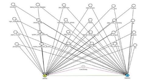
Figure 2 In our tutorial, we illustrated the use of a single data dimension or source to collect proxy information. To demonstrate how multiple proxy data dimensions can be employed, we will now present an example from the literature: the derivation of proxy variables from four data dimensions using the United Kingdom’s Clinical Practice Research Datalink.

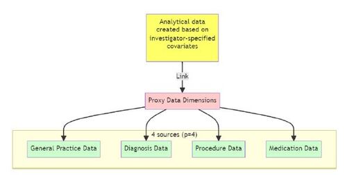
Figure 3 Covariate assessment window applicable for the proxy information.

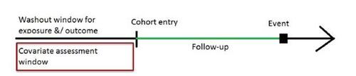
Figure 4 Desnity plot of bias multiplier calculated using the Bross formula for the NHANES dataset.

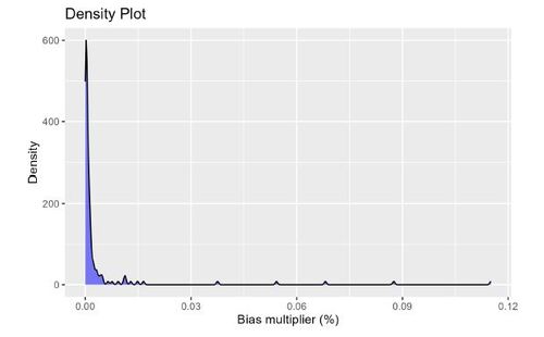
Figure 5 Comparing effect estimates employing various high-dimensional propensity score (hdPS) weighting methods, as well as crude and conventional propensity score (PS) weighting methods using the NHANES dataset. The methods considered include Generalized Linear Model (GLM) or logistic regression (GLM), Least Absolute Shrinkage and Selection Operator (LASSO), Multivariate Adaptive Regression Splines (MARS), Super Learner (SL), PS weighting approach without the inclusion of hdPS variables, and hdPS weighting approach incorporating both investigator-specified covariates and proxies selected by the respective methods.

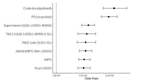
Figure 6 Assessing the impact of choosing different k values (between 10 and 140) to prioritize the recurrence covariates to identify hdPS covariates.

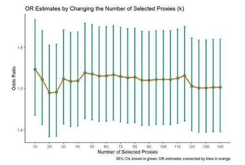
Figure 7 Assessing the impact of choosing different n top prevalent ICD-10-CM codes to identify the candidate empirical covariates.

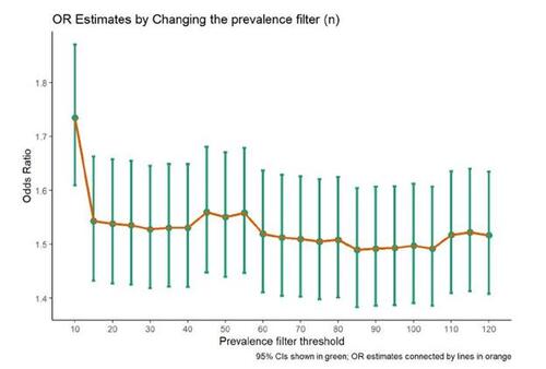
Figure 8 Role of variables in the association of interest, and their usefullness as a variable to be included in the propensity score model. Only confounders and risk factors of outcomes are known to be useful.