Distance Covariance, Independence, and Pairwise Differences

Abstract

Distance covariance (Székely et al. 2007) is a fascinating recent notion, which is popular as a test for dependence of any type between random variables X and Y. This approach deserves to be touched upon in modern courses on mathematical statistics. It makes use of distances of the type $|X-X^{\prime }|$ and $|Y-Y^{\prime }|$, where $(X^{\prime },Y^{\prime })$ is an independent copy of $(X,Y)$. This raises natural questions about independence of variables like $X-X^{\prime }$ and $Y-Y^{\prime }$, about the connection between $\text{Cov}(|X-X^{\prime }|,|Y-Y^{\prime }|)$ and the covariance between doubly centered distances, and about necessary and sufficient conditions for independence. We show some basic results and present a new and nontechnical counterexample to a common fallacy, which provides more insight. We also show some motivating examples involving bivariate distributions and contingency tables, which can be used as didactic material for introducing distance correlation.

Keywords:

• Bivariate distributions
• Correlation
• Doubly centered distances
• Independent random variables

Disclaimer

As a service to authors and researchers we are providing this version of an accepted manuscript (AM). Copyediting, typesetting, and review of the resulting proofs will be undertaken on this manuscript before final publication of the Version of Record (VoR). During production and pre-press, errors may be discovered which could affect the content, and all legal disclaimers that apply to the journal relate to these versions also.

1 Introduction

Independence of random variables is an important and nontrivial topic in probability and statistics. There are many subtleties concerning independence and correlation, see e.g. Mukhopadhyay (2022), Rodgers and Nicewander (1988), and Rousseeuw and Molenberghs (1994). It is often emphasized in class that two real random variables X and Y having zero covariance does not imply their independence. The recent work of Székely et al. (2007) provided a surprising contrast, since the distance covariance they introduced does characterize independence. In our opinion this topic would be a valuable addition to a graduate course on mathematical statistics, because distance covariance is a general method with interesting properties and wide ranging applications, for instance in variable selection (Chen et al. 2018), sparse contingency tables (Zhang 2019), independent component analysis (Matteson and Tsay 2017), and time series (Davis et al. 2018). It can be computed fast (Huo and Székely 2016; Chaudhuri and Hu 2019), and there are interesting connections with other dependence measures (Edelmann and Goeman 2022). Its robustness to outliers was studied recently (Leyder et al. 2024).

The formulation of the distance covariance, described in Section 3, is very simple but contains some subtleties that often give rise to misunderstandings. It is based on pairwise differences $X-X^{\prime }$ and $Y-Y^{\prime }$, where $(X^{\prime },Y^{\prime })$ is an independent copy of $(X,Y)$. In order to provide a context for the role of these pairwise differences, we establish some connections between independence of X and Y and independence relations involving $X-X^{\prime }$ and $Y-Y^{\prime }$. We have not found these results in the literature, and we believe they could provide a pedagogic background.

We also construct an elementary counterexample to a common misunderstanding, with the aim of clarifying why the distance covariance approach requires “double centering” of the interpoint distances $|X-X^{\prime }|$ and $|Y-Y^{\prime }|$.

Most of the material in this paper is accessible to students who took an introductory course in probability and statistics. Only the statements of Proposition 1(b) and Proposition 2(c) and the proofs in the Appendix require knowledge of characteristic functions, but this is not needed to follow the examples.

2 Some results on pairwise differences

Let us denote independence of a pair of real random variables as $X\perp \perp Y$. We start by looking at pairwise differences of only one of the variables, say X. We consider an independent copy $X^{\prime }$ of X, that is, $X^{\prime }\sim X$ and $X^{\prime }\perp \perp (X,Y)$. Then the following implications hold.

Proposition 1 .

For a pair of random variables $(X,Y)$ it holds that

(a) $X\perp \perp Y$ implies $(X-X^{\prime })\perp \perp Y$ .

(b) If the characteristic function of X has no roots or only isolated roots, or the

characteristic function of $(X,Y)$ is analytic, then $(X-X^{\prime })\perp \perp Y$ implies $X\perp \perp Y$ .

The proof can be found in the Appendix. Part (a) is general, as it does not require any conditions on X or Y, such as the existence of certain moments. Part (b) is a bit more involved. We have been unable to find this proposition in the literature, but since part (a) is straightforward we expect that it is known.

The conditions on the characteristic functions in part (b) of Proposition 1 look quite stringent, but there are many relevant cases. The characteristic functions of the Gaussian, Student, exponential, Poisson, chi-square, Gamma, Laplace, logistic, Cauchy, and stable distributions have no roots. Distributions whose characteristic functions have non-isolated zeroes are unusual, but some examples do exist, see e.g. Ushakov (1999), page 265. The alternative condition that ${\varphi }_{(X,Y)}$ is analytic is satisfied whenever X and Y are bounded, see e.g. Berezin (2016), page 147.

Next we consider pairwise differences of both X and Y. For this we take an independent copy $(X^{\prime },Y^{\prime })$ of $(X,Y)$, that is, $(X^{\prime },Y^{\prime })\sim (X,Y)$ and $(X^{\prime },Y^{\prime })\perp \perp (X,Y)$.

Proposition 2 .

For a pair of random variables $(X,Y)$ it holds that

(a) $X\perp \perp Y$ implies $(X-X^{\prime })\perp \perp (Y-Y^{\prime })$ .

(b) $(X-X^{\prime })\perp \perp (Y-Y^{\prime })$ and $(X-X^{\prime })\perp \perp Y$ together imply $X\perp \perp Y$.

(c) If $(X,Y)$ is symmetric and its characteristic function has no roots or is analytic,

$(X-X^{\prime })\perp \perp (Y-Y^{\prime })$ implies $X\perp \perp Y$.

We could not find these results in the literature either, and in our opinion they could provide a useful background when the notion of distance covariance is taught. Also, parts (a) of Propositions 1 and 2 could be used as exercises in a chapter on characteristic functions. Together with the partial converses in these propositions they would make a viable homework assignment, as long as the exact statements of the propositions are provided, and perhaps also those of the lemmas in the Appendix.

It is worth noting that the converse of part (a) of Proposition 2 does not hold without further conditions, because there exists a nontrivial counterexample (Gabor Székely 2024, personal communication). Therefore also the converse of Proposition 1(a) cannot hold without further conditions, or else we could prove the converse of Proposition 2(a) by applying the converse of Proposition 1(a) twice.

3 Connection with distance covariance

If $X\perp \perp Y$ we obtain from Proposition 2(a) that $(X-X^{\prime })\perp \perp (Y-Y^{\prime })$. But then it follows that also $|X-X^{\prime }|\perp \perp |Y-Y^{\prime }|$, since the absolute value is a continuous function. If X and Y have second moments, that is, $\mathbb{E}[X^2]$ and $\mathbb{E}[Y^2]$ are finite, also $\mathbb{E}[|X-X^{\prime }{|}^2]$ and $\mathbb{E}[|Y-Y^{\prime }{|}^2]$ are finite. Therefore the covariance of $|X-X^{\prime }|$ and $|Y-Y^{\prime }|$ exists as well, and since $|X-X^{\prime }|\perp \perp |Y-Y^{\prime }|$ we have(1) $$\text{Cov}(|X-X^{\prime }|,|Y-Y^{\prime }|)=0.$$(1)

Therefore, when the second moments of X and Y exist, $\text{Cov}(|X-X^{\prime }|,|Y-Y^{\prime }|)=0$ is a necessary condition for $X\perp \perp Y$. However, it is not a sufficient condition. In order to illustrate this, we set out to construct a simple counterexample.

Example 1. The smallest example we were able to produce is a probability distribution on 4 points in the plane. Table 1 lists the coordinates of $(X,Y)$, and the 4 points are plotted in the top panel of Figure 1. Note that X and Y are uncorrelated but not independent, since the distribution of $Y|X=x$ depends on x. The $Y\sim X$ regression line is horizontal. The resulting distribution of $(|X-X^{\prime }|,|Y-Y^{\prime }|)$ contains 5 points, given in the middle panel of Table 1 with their probabilities, and plotted in the bottom left panel of Figure 1. It is easily verified that $\text{Cov}(|X-X^{\prime }|,|Y-Y^{\prime }|)$ is exactly zero. So this is an example with non-independent X and Y for which $\text{Cov}(|X-X^{\prime }|,|Y-Y^{\prime }|)=0.$

Székely et al. (2007) proposed to use another function. Instead of the interpoint distances $|X-X^{\prime }|$ above, they compute their doubly centered version given by(2) $$\begin{array}{cc}\Delta (X,X^{\prime })=|X-X^{\prime }|-{\mathbb{E}}_{X^{″}}\left[\right|X-X^{″}\left|\right]\hfill & \hfill \\ -{\mathbb{E}}_{X^{″}}\left[\right|X^{″}-X^{\prime }\left|\right]+{\mathbb{E}}_{X^{″},X^{″\prime }}\mathbb{E}\left[\right|X^{″}-X^{″\prime }\left|\right]\hfill & \hfill \end{array}$$(2)

where $X^{″}$ and $X^{″\prime }$ are also independent copies of X. For $\Delta (X,X^{\prime })$ to exist it is necessary that $E[|X|]$ is finite. Note that $\Delta (X,X^{\prime })=\Delta (X^{\prime },X)$ is not a distance itself, since it also takes on negative values. Moreover, ${\mathbb{E}}_X[\Delta (X,X^{\prime })]$ is zero, and the same holds for ${\mathbb{E}}_{X^{\prime }}[\Delta (X,X^{\prime })]$ and ${\mathbb{E}}_{X,X^{\prime }}[\Delta (X,X^{\prime })]$. This explains the name ‘doubly centered’. It turns out that the second moments of $\Delta (X,X^{\prime })$ exist as well.

If also $\mathbb{E}[|Y|]$ is finite, Székely et al. (2007) compute what they call the distance covariance of X and Y, given by(3) $$\text{dCov}(X,Y):=\text{Cov}(\Delta (X,X^{\prime }),\Delta (Y,Y^{\prime })).$$(3)

(In fact they took the square root of the right hand side, but we prefer not to because the units of (3) are those of X times Y.) They proved the amazing result that when the first moments of X and Y exist, it holds that(4) $$X\perp \perp Y\iff \text{dCov}(X,Y)=0.$$(4)

This yields a necessary and sufficient condition for independence. The implication $�$ is not obvious at all, and was proved by complex analysis. Their work also made it clear that always $\text{dCov}(X,Y)\mathrm{⩾}0$ because they can write $\text{dCov}(X,Y)$ as an integral of a nonnegative function.

The bottom panel of Table 1 lists the coordinates of the $(\Delta (X,X^{\prime }),\Delta (Y,Y^{\prime }))$ and their probabilities, and these points are plotted in the bottom right panel of Figure 1. Note that we now have 7 points instead of 5. Indeed, the atom $\{(a,a),(b,b),(c,c),(d,d)\}$ of $(|X-X^{\prime }|,|Y-Y^{\prime }|)$ has split into three atoms of $(\Delta (X,X^{\prime }),\Delta (Y,Y^{\prime }))$. Even though all four pairs have the same $(X-X^{\prime },Y-Y^{\prime })=(0,0)$, they can obtain different $(\Delta (X,X^{\prime }),\Delta (Y,Y^{\prime }))$ because different means were subtracted from their $|X-X^{\prime }|=0$ and $|Y-Y^{\prime }|=0$. This implies that the doubly centered distance $\Delta (X,X^{\prime })$ cannot be written as a function of $X-X^{\prime }$.

In spite of the name ‘distance covariance’, dCov is thus fundamentally different from the covariance of distances in (1). As we just saw, dCov is not a function of the pairwise differences $X-X^{\prime }$ and $Y-Y^{\prime }$ alone: to compute $\Delta (x,x^{\prime })$ we need to know the actual values of x and $x^{\prime }$. So the arrow $\Rightarrow$ in (4) is not an immediate consequence of $|X-X^{\prime }|\perp \perp |Y-Y^{\prime }|$ or even of the fact that $X-X^{\prime }\perp \perp Y-Y^{\prime }$ , instead it is truly derived from $X\perp \perp Y$. (If $\Delta (X,X^{\prime })$ were a function of $X-X^{\prime }$ it would follow from $(X-X^{\prime })\perp \perp (Y-Y^{\prime })$ that $\text{dCov}(X,Y)=0$ and hence $X\perp \perp Y$, which we know is not true in general.)

In the example we obtain exactly $\text{dCov}(X,Y)=0.1>0$, which confirms the dependence of X and Y. The example thus illustrates that the double centering in $\text{dCov}(X,Y)$ is necessary to characterize independence, since without it we obtained $\text{Cov}(|X-X^{\prime }|,|Y-Y^{\prime }|)=0$ which provided no clue about the dependence of X and Y.

The regression line in the bottom right panel of Figure 1 is not horizontal but goes up. Its slope must be positive or zero because it is a positive multiple of $\text{dCov}(X,Y)$, which we know is always nonnegative. The regression line also has to pass through the origin $(0,0)$, because the doubly centered distances of X as well as Y have zero mean, so the average of the points in this plot is the origin. In this tiny example the regression line also happens to pass through one of the points in the plot, but that is a coincidence. The line does not have to pass through any point, as can be verified by e.g. changing the first x-coordinate of the original data from -1.0 to -1.5 .

Székely et al. (2007) also derived a different expression for dCov. Working out the covariance in (3) yields $4\times 4=16$ terms, that exist when X and Y also have second moments. With elementary manipulations and a lot of patience these terms can be reduced to three:$$\begin{array}{cc}\text{dCov}(X,Y)=\mathbb{E}\left[\right|X-X^{\prime }\left|\right|Y-Y^{\prime }\left|\right]+\mathbb{E}\left[\right|X-X^{\prime }\left|\right]\mathbb{E}\left[\right|Y-Y^{\prime }\left|\right]\hfill & \hfill \\ -2\mathbb{E}\left[\right|X-X^{\prime }\left|\right|Y-Y^{″}\left|\right].\hfill & \hfill \end{array}$$

Combining the first term on the right with minus the second, and the third with twice the second, Székely and Rizzo (2023) obtain$$\text{dCov}(X,Y)=\text{Cov}(|X-X^{\prime }|,|Y-Y^{\prime }|)-2\text{Cov}(|X-X^{\prime }|,|Y-Y^{″}|)$$

which connects dCov with the covariance of distances in (1). Since we have seen that $X\perp \perp Y$ implies that $\text{Cov}(|X-X^{\prime }|,|Y-Y^{\prime }|)=0$, the only way that X and Y can be independent is when both terms on the right hand side are zero. In the example $\text{Cov}(|X-X^{\prime }|,|Y-Y^{\prime }|)=0$ but X and Y are dependent, so the second term has to be nonzero, and indeed $\text{Cov}(|X-X^{\prime }|,|Y-Y^{″}|)=-0.05$ .

4 Distance correlation and finite samples

Since the units of $\text{dCov}(X,Y)$ are those of X times Y, and $\text{dCov}(aX,bY)=ab\hspace{0.17em}\text{dCov}(X,Y)$, one often uses the unitless distance correlation defined as(5) $$\text{dCor}(X,Y)=\frac{\text{dCov}(X,Y)}{\sqrt{\text{dCov}(X,X)\text{dCov}(Y,Y)}}$$(5)

which always lies between 0 and 1. Note that the conventional definition is the square root of (5).

So far we have worked with population distributions, but dCov and dCor can also be used for finite samples. One can simply apply them to the empirical distribution of the sample. In particular, for a univariate sample $X_n=(x_1,\dots ,x_n)$ we denote $d_{ij}:=|x_i-x_j|$ for $i,j=1,\dots ,n$ as well as(6) $$\overline{d_{i·}}=\frac{1}{n}\sum _{j=1}^n{d}_{ij}\mathrm{\hspace{1em}}\mathrm{\hspace{1em}}\overline{d_{·j}}=\frac{1}{n}\sum _{i=1}^n{d}_{ij}\mathrm{\hspace{1em}}\mathrm{\hspace{1em}}\overline{d_{··}}=\frac{1}{n^2}\sum _{i,j=1}^n{d}_{ij}\hspace{0.17em}\hspace{0.17em}.$$(6)

Double centering yields the values$${\Delta }_{ij}^{X_n}:=d_{ij}-\overline{d_{i·}}-\overline{d_{·j}}+\overline{d_{··}}$$

so that ${\sum }_{j=1}^n{\Delta }_{ij}^{X_n}=0$ for all i and ${\sum }_{i=1}^n{\Delta }_{ij}^{X_n}=0$ for all j. The dCov of a bivariate sample is then defined as(7) $$\text{dCov}(X_n,Y_n)=\frac{1}{n^2}\sum _{i,j=1}^n{\Delta }_{ij}^{X_n}{\Delta }_{ij}^{Y_n}\hspace{0.17em}\hspace{0.17em}.$$(7)

The dCor of a bivariate sample is analogous to (5). When based on an i.i.d. sample of size n from a pair of random variables $(X,Y)$ with first moments, the finite-sample $\text{dCov}(X_n,Y_n)$ converges almost surely to $\text{dCov}(X,Y)$ when $n\to \infty$ (Székely et al. 2007).

5 Examples

The material in this section and the next one can be used as exercises for students, in a lab session or a homework assignment.

Example 2. The distance covariance can be applied to contingency tables. For instance, $2\times 2$ contingency tables can be modeled by Bernoulli variables X and Y, that can only take on the values 0 and 1. We denote their joint probability as $p_{ij}=P(X=i,Y=j)$ and the marginal probabilities as $p_{i·}=p_{i0}+p_{i1}$ and $p_{·j}=p_{0j}+p_{1j}$ . It can be verified that(8) $$\text{dCov}(X,Y)=\sum _{i=0}^1\sum _{j=0}^1{(p_{ij}-p_{i·}{p}_{·j})}^2.$$(8)

Therefore $\text{dCov}(X,Y)=0$ iff $p_{ij}=p_{i·}{p}_{·j}$ for all $i,j=0,1$, which is equivalent to $X\perp \perp Y$. Note that (8) is similar to Pearson’s chi-square statistic, but not identical. If we divide the chi-square statistic by the sample size, and let the sample size grow, it converges to the population version$$\sum _{i=0}^1\sum _{j=0}^1{(\frac{p_{ij}-p_{i·}{p}_{·j}}{p_{i·}{p}_{·j}})}^2$$

which is not equivalent to (8). It is not too difficult to derive that(9) $$\text{Cov}(|X-X^{\prime }|,|Y-Y^{\prime }|)=2(p_{00}{p}_{11}+p_{01}{p}_{10}-2p_{0·}{p}_{1·}{p}_{·0}{p}_{·1}).$$(9)

Now it is easy to see that $X\perp \perp Y$ implies that (9) becomes zero. But it is not true the other way around. A counterexample is given by $(p_{00},p_{01},p_{10},p_{11})=(10,5,14,11)/40$. This zeroes $\text{Cov}(|X-X^{\prime }|,|Y-Y^{\prime }|)$, but X and Y are not independent and $\text{dCov}(X,Y)=0.025$ is strictly positive. (Unlike Example 1 in Table 1, here the plain $\text{Cov}(X,Y)$ is not zero.)

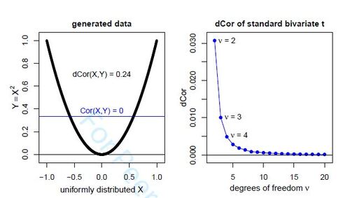
Example 3. The main advantage of dCor over the usual product-moment correlation Cor is that from $\text{dCor}(X,Y)=0$ it follows that $X\perp \perp Y$. Most introductory statistics books stress that this does not hold for Cor. A typical illustrative example is to take a univariate variable X with a distribution that has a second moment and is symmetric about zero, and to put $Y=X^2$. (If a bivariate density is desired, one can add a Gaussian error term to Y.) Let us take the simple case where X follows the uniform distribution on $[-1,1]$. Clearly X and Y are dependent, but by symmetry $\text{Cor}(X,Y)=0$. However, we will see that $\text{dCor}(X,Y)$ is strictly positive.

The computation of $\text{dCor}(X,Y)$ offers an opportunity for carrying out a simple numerical experiment. First we have to generate a sample of size n from this bivariate distribution. This is easy, for instance in R we can run X = runif(n,min=-1,max = 1) followed by Y = X^2 . This yields the left panel of Figure 2, in which the horizontal regression line illustrates that the classical correlation $\text{Cor}(X,Y)$ is zero. To compute the sample distance correlation we can use the R package energy (Rizzo and Székely 2022) or the package dccpp (Berrisch 2023). In the first case we run energy::dcor2d(X,Y) which uses the algorithm of Huo and Székely (2016), and in the second case the command is dccpp::dcor(X,Y)^2 which carries out the algorithm of Chaudhuri and Hu (2019). Both algorithms for dCor are very fast as their computation time is only $O(n\hspace{0.17em}\log \hspace{0.17em}(n))$, and they do not store the $n\times n$ matrices of all ${\Delta }_{ij}^{X_n}$ and ${\Delta }_{ij}^{Y_n}$ . When we let n grow, the answer quickly converges to approximately $0.2415>0$. The result stabilizes even faster if we use an equispaced set X = seq(from=-1,to = 1,by = 2/(n-1)), so the computation becomes a crude numerical integration.

Example 4. In the previous example the left panel of Figure 2 immediately reveals the dependence, because the conditional expectation $E[Y|X=x]=x^2$ depends on x. But there are more subtle situations, where for instance the conditional expectation is constant but some other moment is not. A nice example is the bivariate t-distribution. When its center is $(0,0)$ and its scatter matrix is the identity matrix, it is called the standard bivariate t-distribution with density(10) $$f(x,y)=\frac{1}{2\pi }{(1+\frac{x^2+y^2}{\nu })}^{-(\nu +2)/2}$$(10)

where $\nu$ is the degrees of freedom parameter. The marginal distribution of Y is the usual univariate t-distribution with center 0 given by(11) $$f_t(y;s^2,\nu )=\frac{c(\nu )}{s}{(1+\frac{{(y/s)}^2}{\nu })}^{-(\nu +1)/2}$$(11)

where $c(\nu )$ is the constant needed to make the density integrate to 1, and the scale parameter s equals 1 here. In general $\text{Var}(Y)=s^2\nu /(\nu -2)$ when $\nu >2$. A plot of the bivariate density (10) looks a lot like that of the standard bivariate Gaussian distribution, with circular symmetry. When $\nu >2$ the correlation $\text{Cor}(X,Y)$ exists and is zero. But whereas X and Y are independent in the standard Gaussian setting, they are no longer here, since the bivariate density (10) does not equal the product of the marginal densities of X and Y. The conditional density of Y given $X=x$ is now(12) $$f(y|X=x)=f_t(y;\frac{\nu +x^2}{\nu +1},\nu +1)$$(12)

(Ding 2016), so it is again a univariate t with center 0, but now with $\nu +1$ degrees of freedom and a scale parameter that depends on x. Due to the increased degrees of freedom, the conditional expectation already exists for $\nu >0$ and equals zero, so it is constant. The conditional variance exists for any $\nu >1$ and equals $(\nu +x^2)/(\nu -1)$. It is thus lowest for $x=0$ and increases with $\left|x\right|$.

We now study the distance correlation of these dependent but uncorrelated variables X and Y. An analytic derivation of $\text{dCov}(X,Y)$ may not be possible, but in R we can easily generate data from the standard bivariate t-distribution by rmvt(n,df = df) where df is the degrees of freedom $\nu$. The function rmvt is in the R package mvtnorm (Genz et al. 2023). We can then compute the distance correlation in exactly the same way as in Example 3 above. Figure 2 shows the resulting estimates of $\text{dCor}(X,Y)$ obtained for $n=$100 000 and $\nu$ ranging from 2 to 20, a computation that took under one minute. The distance correlation goes down to zero for increasing $\nu$, which is understandable because for $\nu \to \infty$ the standard bivariate t-distribution converges to the standard Gaussian distribution, where X and Y are indeed independent.

6 Testing for independence

Now suppose we have an i.i.d. sample $(X_n,Y_n)$ from a bivariate random variable $(X,Y)$, and we want to test the null hypothesis $H_0$ that X and Y are independent. If we know that $(X,Y)$ is bivariate Gaussian, $X\perp \perp Y$ is equivalent to the true parameter ${\Sigma }_{12}$ being zero, where $\Sigma$ is the unknown covariance matrix of $(X,Y)$. In that particular situation $H_0$ can be tested by computing the sample correlation coefficient of $(X_n,Y_n)$ and comparing it to its null distribution for that sample size.

However, in general we do not know whether data come from a Gaussian distribution, and the bivariate point cloud may have a different shape. We have illustrated in Examples 1, 3, and 4 that dependent variables can be uncorrelated, so a test of $\text{Cov}(X,Y)$ would not suffice anyway. What we need is a distribution-free independence test, meaning that it works for any distribution of $(X,Y)$. Since we know that $X\perp \perp Y$ is characterized by $\text{dCov}(X,Y)=0$, a natural idea is to compute the test statistic $\text{dCov}(X_n,Y_n)$ from the sample. Larger values of $\text{dCov}(X_n,Y_n)$ provide more evidence against $H_0$ than smaller values, but how can we compute the p-value when we do not know the kind of distribution that $(X,Y)$ has?

Since all we have is the dataset $(X_n,Y_n)$, this is what we must use. Whatever the distribution of $(X,Y)$, a random permutation of $Y_n$ will be independent of $X_n$ . More formally, if we draw a permutation $\tau$ from the uniform distribution on all $n!$ permutations on $(1,\dots ,n)$, we have $Y_n^{\tau }:=(y_{\tau (1)},\dots ,y_{\tau (n)})\perp \perp X_n$ . If n is very small we can use all possible permutations $\tau$, and otherwise we can draw many of them, say $m=1000$ permutations ${\tau }_1,\dots ,{\tau }_m$ . We can then estimate the p-value by counting how often $\text{dCov}(X_n,Y_n^{{\tau }_m})$ with the permuted $Y_n^{{\tau }_m}$ is larger than the observed $\text{dCov}(X_n,Y_n)$:$$\widehat{p}=\frac{1}{m+1}(\#\{m|\hspace{0.17em}\text{dCov}(X_n,Y_n^{{\tau }_m})>\text{dCov}(X_n,Y_n)\}+1).$$

The $+1$ stems from the fact that the original $Y_n$ corresponds to the identical permutation $(1,\dots ,n)$ and is independent of $X_n$ under $H_0$ , and has the advantage that $\widehat{p}$ cannot become exactly zero, which would be unrealistic.

The permutation test is simple, and it is fast due to the fast algorithms for dCov. Note that it would make no difference if we would replace dCov by dCor, since the denominator ${(\text{dCov}(X_n,X_n)\text{dCov}{(Y_n^{{\tau }_m},Y^{{\tau }_m})}_n)}^{1/2}={(\text{dCov}(X_n,X_n)\text{dCov}(Y_n,Y_n))}^{1/2}$ of dCor is constant, so it is easiest to stick with dCov. Also, it does not matter whether we square dCov or not. More information about testing independence can be found in (Székely and Rizzo 2023). A potential exercise for students would be to generate samples from the bivariate distributions in Example 3 or 4 of Section 5 and compute $\widehat{p}$ for different sample sizes. In that setting they can also estimate the power of the permutation test for a fixed level, for instance by rejecting $H_0$ when $\widehat{p}<0.05$, using simulation.

Supplementary Material. This is an R script that reproduces the examples.

A. Appendix with proofs

In order to prove Proposition 1, it turns out that the following lemma is very helpful.

Lemma 1 .

If $(X,Y)$ is a pair of random variables and we construct an independent copy $X^{\prime }$ of X, that is, $X^{\prime }\sim X$ and $X^{\prime }\perp \perp (X,Y)$, then $(X-X^{\prime })\perp \perp Y$ is equivalent to the condition

$\mathit{for\; all\; t}\hspace{0.17em}\hspace{0.17em}\mathit{with}$ ${\varphi }_{(X,Y)}(t,0)\ne 0:$ $\hspace{0.17em}\hspace{0.17em}{\varphi }_{(X,Y)}(t,v)={\varphi }_{(X,Y)}(t,0){\varphi }_{(X,Y)}(0,v).$ (13)

Proof of Lemma 1.

For the direction $\Rightarrow$ we compute the characteristic functions$$\begin{array}{c}{\varphi }_{(X,-X^{\prime },Y)}(s,t,v)={\varphi }_{-X^{\prime }}(t){\varphi }_{(X,Y)}(s,v)\hfill \\ {\varphi }_{(X-X^{\prime },Y)}(t,v)={\varphi }_{X-X^{\prime }}(t){\varphi }_Y(v)={\varphi }_X(t){\varphi }_{-X^{\prime }}(t){\varphi }_Y(v).\hfill \end{array}$$

On the subset $\{s=t\}$ both left hand sides equal $\mathbb{E}[e^{it(X-X^{\prime })+\mathit{ivY}}]$ so(14) $${\varphi }_{(X,Y)}(t,v){\varphi }_X(-t)={\varphi }_X(t){\varphi }_X(-t){\varphi }_Y(v).$$(14)

Since ${\varphi }_X$ is Hermitian its set of roots is symmetric, so we have that ${\varphi }_X(t)\ne 0\Rightarrow {\varphi }_X(-t)\ne 0$ and in that case ${\varphi }_X(-t)$ cancels in (14), yielding (13).

For the direction $\Leftarrow$ we compute$$\begin{array}{cc}{\varphi }_{(X-X^{\prime },Y)}(t,v)=\mathbb{E}\left[e^{it(X-X^{\prime })+\mathit{ivY}}\right]=\mathbb{E}\left[e^{\mathit{itX}}{e}^{-it{X}^{\prime }}{e}^{\mathit{ivY}}\right]\hfill & \hfill \\ ={\varphi }_{-X^{\prime }}(t){\varphi }_{(X,Y)}(t,v)\hspace{1em}\text{due}\mathrm{ }\text{to}\mathrm{ }{X}^{\prime }\perp \perp (X,Y).\hfill & \hfill \end{array}$$

In this equality we can replace ${\varphi }_{(X,Y)}(t,v)$ by ${\varphi }_X(t){\varphi }_Y(v)$ whenever ${\varphi }_X(-t)\ne 0$, so then(15) $${\varphi }_{(X-X^{\prime },Y)}(t,v)={\varphi }_{X-X^{\prime }}(t){\varphi }_Y(v).$$(15)

But this also holds when ${\varphi }_X(-t)=0$ because then ${\varphi }_{-X^{\prime }}(t){\varphi }_{(X,Y)}(t,v)=0={\varphi }_X(-t){\varphi }_X(t){\varphi }_Y(v)$. Therefore (15) holds unconditionally, hence $(X-X^{\prime })\perp \perp Y$. ▪

Proof of Proposition 1.

For (a) we use the fact that $X\perp \perp Y$ implies ${\varphi }_{(X,Y)}(t,v)={\varphi }_X(t){\varphi }_Y(v)$ for any t and v, which is stronger than condition (13) in Lemma 1, hence $(X-X^{\prime })\perp \perp Y$.

For (b) we also start from condition (13) in Lemma 1. If the characteristic function of X has no roots we always have ${\varphi }_X(-t)\ne 0$ so(16) $${\varphi }_{(X,Y)}(t,v)={\varphi }_X(t){\varphi }_Y(v)\hspace{1em}\mathrm{ }\text{for}\mathrm{ }\text{all}\mathrm{ }(t,v)$$(16)

hence $X\perp \perp Y$.

Suppose that ${\varphi }_X$ does have roots but they are isolated, implying that the non-roots form a dense set. That is, any root t is the limit of a sequence of non-roots $t_n$ for $n\to \infty$. In each $t_n$ we have ${\varphi }_{(X,Y)}(t_n,v)={\varphi }_X(t_n){\varphi }_Y(v)$ by condition (13). Since characteristic functions are absolutely continuous we can pass to the limit, again yielding (16).

If we assume nothing about roots but ${\varphi }_{(X,Y)}$ is analytic, so are ${\varphi }_X(t)={\varphi }_{(X,Y)}(t,0)$ and ${\varphi }_Y(v)={\varphi }_{(X,Y)}(0,v)$. All characteristic functions take the value 1 at the origin, and are absolutely continuous. Therefore there is a $\delta >0$ such that for all $(t,v)$ in the disk $B((0,0),\delta )$ it holds that ${\varphi }_{(X,Y)}(t,v)$ as well as ${\varphi }_X(t)$ and ${\varphi }_Y(v)$ are nonzero. On that disk we can thus divide by ${\varphi }_X(-t)$ in (14), hence ${\varphi }_{(X,Y)}(t,v)={\varphi }_X(t){\varphi }_Y(v)$ holds on it. Since ${\varphi }_X(t)$ and ${\varphi }_Y(v)$ are analytic, so is their product. By analytic continuation (16) holds, so again $X\perp \perp Y$. ▪

We now consider pairwise differences of both variables X and Y. This requires a second lemma.

Lemma 2 .

If $(X,Y)$ is a pair of random variables and we construct an independent copy $(X^{\prime },Y^{\prime })$ of it, that is, $(X^{\prime },Y^{\prime })\sim (X,Y)$ and $(X^{\prime },Y^{\prime })\perp \perp (X,Y)$, then $(X-X^{\prime })\perp \perp (Y-Y^{\prime })$ is equivalent to the condition (17) $$|{\varphi }_{(X,Y)}(t,v)|=|{\varphi }_{(X,Y)}(t,0)||{\varphi }_{(X,Y)}(0,v)|\hspace{1em}\mathrm{ }\text{for}\mathrm{ }\text{all}\mathrm{ }(t,v).$$(17)

Proof of Lemma 2.

For the direction $\Rightarrow$ we compute the characteristic functions$$\begin{array}{c}{\varphi }_{(X,-X^{\prime },Y,-Y^{\prime })}(s,t,u,v)={\varphi }_{(X,Y)}(s,u){\varphi }_{(-X^{\prime },-Y^{\prime })}(t,v)={\varphi }_{(X,Y)}(s,u){\varphi }_{(X,Y)}(-t,-v)\hfill \\ {\varphi }_{(X-X^{\prime },Y-Y^{\prime })}(t,v)={\varphi }_{X-X^{\prime }}(t){\varphi }_{Y-Y^{\prime }}(v)={\varphi }_X(t){\varphi }_{-X^{\prime }}(t){\varphi }_Y(v){\varphi }_{-Y^{\prime }}(v).\hfill \end{array}$$

On the subset $\{s=t,u=v\}$ both left hand sides equal $\mathbb{E}[e^{it(X-X^{\prime })+iv(Y-Y^{\prime })}]$. Therefore$$|{\varphi }_{(X,Y)}(t,v){|}^2={\varphi }_{(X,Y)}(t,v){\varphi }_{(X,Y)}(-t,-v)={\varphi }_{X-X^{\prime }}(t){\varphi }_{Y-Y^{\prime }}(v)=|{\varphi }_X(t){|}^2|{\varphi }_Y(v){|}^2.$$

For the direction $\Leftarrow$ we compute$$\begin{array}{cc}{\varphi }_{(X-X^{\prime },Y-Y^{\prime })}(t,v)=\mathbb{E}\left[e^{\mathit{itX}}{e}^{-it{X}^{\prime }}{e}^{\mathit{ivY}}{e}^{-iv{Y}^{\prime }}\right]\hfill & \hfill \\ =\mathbb{E}\left[e^{\mathit{itX}+\mathit{ivY}}\right]\mathbb{E}\left[e^{-it{X}^{\prime }-iv{Y}^{\prime }}\right]\hspace{1em}\text{due}\mathrm{ }\text{to}\mathrm{ }(X^{\prime },Y^{\prime })\perp \perp (X,Y)\hfill & \hfill \\ ={\varphi }_{(X,Y)}(t,v)\overline{{\varphi }_{(X,Y)}(t,v)}=|{\varphi }_{(X,Y)}(t,v){|}^2\hfill & \hfill \\ =|{\varphi }_X(t){|}^2|{\varphi }_Y(v){|}^2\hspace{1em}\text{from} (17)\hfill & \hfill \\ ={\varphi }_{X-X^{\prime }}(t){\varphi }_{Y-Y^{\prime }}(v)\hfill & \hfill \end{array}$$

hence $(X-X^{\prime })\perp \perp (Y-Y^{\prime })$. □

Proof of Proposition 2.

For (a) we use the fact that $X\perp \perp Y$ implies that ${\varphi }_{(X,Y)}(t,v)={\varphi }_X(t){\varphi }_Y(v)$ for any t and v, hence $|{\varphi }_{(X,Y)}(t,v)|=|{\varphi }_X(t)||{\varphi }_Y(v)|$ which is condition (17) in Lemma 2, so $(X-X^{\prime })\perp \perp (Y-Y^{\prime })$.

For (b), $(X-X^{\prime })\perp \perp Y$ implies ${\varphi }_{(X,Y)}(t,v)={\varphi }_X(t){\varphi }_Y(v)$ for all t with ${\varphi }_X(t)\ne 0$ by Lemma 1. In the remaining points $(t,v)$ it holds that ${\varphi }_X(t)=0$ and then $|{\varphi }_{(X,Y)}(t,v)|=|{\varphi }_X(t)||{\varphi }_Y(v)|=0$ by condition (17) of Lemma 2, so ${\varphi }_{(X,Y)}(t,v)=0={\varphi }_X(t){\varphi }_Y(v)$ as well. The combination yields (16), hence $X\perp \perp Y$.

Part (c). By symmetry of $(X,Y)$ and hence of X and Y we know that ${\varphi }_{(X,Y)}(t,v)$ as well as ${\varphi }_X(t)$ and ${\varphi }_Y(v)$ are real and even, hence condition (17) yields(18) $${\varphi }_{(X,Y)}^2(t,v)={\varphi }_X^2(t){\varphi }_Y^2(v).$$(18)

If ${\varphi }_{(X,Y)}(t,v)$ has no roots, it follows from ${\varphi }_{(X,Y)}(0,0)=1$ and continuity of ${\varphi }_{(X,Y)}$ that always ${\varphi }_{(X,Y)}(t,v)>0$. Therefore also ${\varphi }_X(t)={\varphi }_{(X,Y)}(t,0)>0$ and ${\varphi }_Y(v)={\varphi }_{(X,Y)}(0,v)>0$. Taking square roots on both sides of (18) yields (16), hence $X\perp \perp Y$.

If, on the other hand, ${\varphi }_{(X,Y)}$ is analytic, so are ${\varphi }_X(t)={\varphi }_{(X,Y)}(t,0)$ and ${\varphi }_Y(v)={\varphi }_{(X,Y)}(0,v)$. All characteristic functions take the value 1 at the origin, and are absolutely continuous. Therefore there is a $\delta >0$ such that for all $(t,v)$ in the disk $B((0,0),\delta )$ it holds that ${\varphi }_{(X,Y)}(t,v)$ as well as ${\varphi }_X(t)$ and ${\varphi }_Y(v)$ are strictly positive. On that disk we can thus take square roots of (18), yielding ${\varphi }_{(X,Y)}(t,v)={\varphi }_X(t){\varphi }_Y(v)$ on it. Since ${\varphi }_X(t)$ and ${\varphi }_Y(v)$ are analytic, so is their product. By analytic continuation the equality must hold everywhere, yielding (16) so again $X\perp \perp Y$. □

Table 1: Example 1: $\text{Cov}(|X-X^{\prime }|,|Y-Y^{\prime }|)=0$ but X and Y are dependent.

atom	X	Y	probability
a	−1	1	1/4
b	1	1	1/4
c	0	0.6	1/4
d	0	−1	1/4
atom	$|X-X^{\prime }|$	$|Y-Y^{\prime }|$	probability
$(a,a),(b,b),(c,c),(d,d)$	0	0	1/4
$(c,d)$	0	1.6	1/8
$(a,c),(b,c)$	1	0.4	1/4
$(a,d),(b,d)$	1	2	1/4
$(a,b)$	2	0	1/8
atom	$\Delta (X,X^{\prime })$	$\Delta (Y,Y^{\prime })$	probability
$(a,a),(b,b)$	−1.25	−0.40	1/8
$(d,d)$	−0.25	−2.00	1/16
$(c,c)$	−0.25	−0.40	1/16
$(c,d)$	−0.25	0.40	1/8
$(a,c),(b,c)$	0.25	0.00	1/4
$(a,d),(b,d)$	0.25	0.80	1/4
$(a,b)$	0.75	−0.40	1/8

Figure 1: Example with a distribution on 4 points, from Table 1. Top: plot of Y versus X. Bottom left: plot of pairwise distances $|Y-Y^{\prime }|$ of Y versus those of X. Bottom right: doubly centered distances $\Delta (Y,Y^{\prime })$ of Y versus those of X.

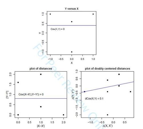
Figure 2: Left: dependent variables generated in Example 3, with horizontal regression line illustrating that X and Y are uncorrelated. Right: Plot of the distance correlation of the standard bivariate t-distribution in Example 4, for a range of $\nu$.