On the second-order asymptotical regularization of linear ill-posed inverse problems

ABSTRACT

In this paper, we establish an initial theory regarding the second-order asymptotical regularization (SOAR) method for the stable approximate solution of ill-posed linear operator equations in Hilbert spaces, which are models for linear inverse problems with applications in the natural sciences, imaging and engineering. We show the regularizing properties of the new method, as well as the corresponding convergence rates. We prove that, under the appropriate source conditions and by using Morozov's conventional discrepancy principle, SOAR exhibits the same power-type convergence rate as the classical version of asymptotical regularization (Showalter's method). Moreover, we propose a new total energy discrepancy principle for choosing the terminating time of the dynamical solution from SOAR, which corresponds to the unique root of a monotonically non-increasing function and allows us to also show an order optimal convergence rate for SOAR. A damped symplectic iterative regularizing algorithm is developed for the realization of SOAR. Several numerical examples are given to show the accuracy and the acceleration effect of the proposed method. A comparison with other state-of-the-art methods are provided as well.

COMMUNICATED BY:

• Michael Klibanov

KEYWORDS:

• Linear ill-posed problems
• asymptotical regularization
• second-order method
• convergence rate
• source condition
• index function
• qualification
• discrepancy principle

AMS SUBJECT CLASSIFICATIONS:

• 47A52
• 65J20
• 65F22
• 65R30

1. Introduction

We are interested in solving linear operator equations, (1) $Ax=y,$(1) where A is an injective and compact linear operator acting between two infinite dimensional Hilbert spaces $\mathcal{X}$ and $\mathcal{Y}$. For simplicity, we denote by $⟨\cdot ,\cdot ⟩$ and $\parallel \cdot \parallel$ the inner products and norms, respectively, for both Hilbert spaces. Since A is injective, the operator equation (1(1) $Ax=y,$(1) ) has a unique solution $x^{†}\in \mathcal{X}$ for every y from range $\mathcal{R}\left(A\right)$ of the linear operator A. In this context, $\mathcal{R}\left(A\right)$ is assumed to be an infinite dimensional subspace of $\mathcal{Y}$.

Suppose that, instead of the exact right-hand side $y=A{x}^{†}$, we are given noisy data $y^{\delta }\in \mathcal{Y}$ obeying the deterministic noise model $\parallel y^{\delta }-y\parallel \le \delta$ with noise level $\delta >0$. Since A is compact and $\dim \left(\mathcal{R}\right(A\left)\right)=\mathrm{\infty }$, we have $\mathcal{R}\left(A\right)\ne \overline{\mathcal{R}\left(A\right)}$ and the problem (1(1) $Ax=y,$(1) ) is ill-posed. Therefore, regularization methods should be employed for obtaining stable approximate solutions.

Loosely speaking, two groups of regularization methods exist: variational regularization methods and iterative regularization methods. Tikhonov regularization is certainly the most prominent variational regularization method (cf., e.g. [1]), while the Landweber iteration is the most famous iterative regularization approach (cf., e.g. [2,3]). In this paper, our focus is on the latter, since from a computational viewpoint the iterative approach seems more attractive, especially for large-scale problems.

For the linear problem (1(1) $Ax=y,$(1) ), the Landweber iteration is defined by (2) $x_{k+1}=x_k+\mathrm{\Delta }t{A}^{\ast }(y^{\delta }-A{x}_k),\mathrm{\Delta }t\in (0,2/\parallel A{\parallel }^2),$(2) where $A^{\ast }$ denotes the adjoint operator of A. We refer to [2, Section 6.1] for the regularization property of the Landweber iteration. The continuous analogue of (2(2) $x_{k+1}=x_k+\mathrm{\Delta }t{A}^{\ast }(y^{\delta }-A{x}_k),\mathrm{\Delta }t\in (0,2/\parallel A{\parallel }^2),$(2) ) can be considered as a first-order evolution equation in Hilbert spaces (3) $\dot{x}\left(t\right)+A^{\ast }Ax\left(t\right)=A^{\ast }{y}^{\delta }$(3) if an artificial scalar time t is introduced, and $\mathrm{\Delta }t\to 0$ in (2(2) $x_{k+1}=x_k+\mathrm{\Delta }t{A}^{\ast }(y^{\delta }-A{x}_k),\mathrm{\Delta }t\in (0,2/\parallel A{\parallel }^2),$(2) ). Here and later on, we use Newton's conventions for the time derivatives. The formulation (3(3) $\dot{x}\left(t\right)+A^{\ast }Ax\left(t\right)=A^{\ast }{y}^{\delta }$(3) ) is known as Showalter's method, or asymptotic regularization [4,5]. The regularization property of (3(3) $\dot{x}\left(t\right)+A^{\ast }Ax\left(t\right)=A^{\ast }{y}^{\delta }$(3) ) can be analysed through a proper choice of the terminating time. Moreover, it has been shown that by using Runge–Kutta integrators, all of the properties of asymptotic regularization (3(3) $\dot{x}\left(t\right)+A^{\ast }Ax\left(t\right)=A^{\ast }{y}^{\delta }$(3) ) carry over to its numerical realization [6].

From a computational viewpoint, the Landweber iteration, as well as the steepest descent method and the minimal error method, is quite slow. Therefore, in practice accelerating strategies are usually used; see [3,7] and references therein for details.

Over the last few decades, besides the first-order iterative methods, there has been increasing evidence to show that the discrete second-order iterative methods also enjoy remarkable acceleration properties for ill-posed inverse problems. The well-known methods are the Levenberg–Marquardt method [8], the iteratively regularized Gauss–Newton method [9], the ν-method [2, Section 6.3], and the Nesterov acceleration scheme [10]. Recently, a more general second-order iterative method – the two-point gradient method – has been developed in [11]. In order to understand better the intrinsic properties of the discrete second-order iterative regularization, we consider in this paper the continuous version (4) $\begin{array}{rl}& \ddot{x}\left(t\right)+\eta \dot{x}\left(t\right)+A^{\ast }Ax\left(t\right)=A^{\ast }{y}^{\delta },\\ & x\left(0\right)=x_0,\dot{x}\left(0\right)={\dot{x}}_0\end{array}$(4) of the second-order iterative method in the form of an evolution equation, where $x_0\in \mathcal{X}$ and ${\dot{x}}_0\in \mathcal{X}$ are the prescribed initial data and $\eta >0$ is a constant damping parameter.

From a physical viewpoint, the system (4(4) $\begin{array}{rl}& \ddot{x}\left(t\right)+\eta \dot{x}\left(t\right)+A^{\ast }Ax\left(t\right)=A^{\ast }{y}^{\delta },\\ & x\left(0\right)=x_0,\dot{x}\left(0\right)={\dot{x}}_0\end{array}$(4) ) describes the motion of a heavy ball that rolls over the graph of the residual norm square functional $\mathrm{\Phi }\left(x\right)=\parallel y^{\delta }-Ax{\parallel }^2$ and that keeps rolling under its own inertia until friction stops it at a critical point of $\mathrm{\Phi }\left(x\right)$. This nonlinear oscillator with damping, which is called the Heavy Ball with Friction (HBF) system, has been considered by several authors from an optimization viewpoint, establishing different convergence results and identifying the circumstances under which the rate of convergence of HBF is better than the one of the first-order methods; see [12–14]. Numerical algorithms based on (4(4) $\begin{array}{rl}& \ddot{x}\left(t\right)+\eta \dot{x}\left(t\right)+A^{\ast }Ax\left(t\right)=A^{\ast }{y}^{\delta },\\ & x\left(0\right)=x_0,\dot{x}\left(0\right)={\dot{x}}_0\end{array}$(4) ) for solving some special problems, e.g. inverse source problems in partial differential equations, large systems of linear equations, and the nonlinear Schrödinger problem, etc., can be found in [15–18]. The main goal of this paper is the intrinsic structure analysis of the theory of the second-order iterative regularization and the development of new iterative regularization methods based on the framework (4(4) $\begin{array}{rl}& \ddot{x}\left(t\right)+\eta \dot{x}\left(t\right)+A^{\ast }Ax\left(t\right)=A^{\ast }{y}^{\delta },\\ & x\left(0\right)=x_0,\dot{x}\left(0\right)={\dot{x}}_0\end{array}$(4) ).

The remainder of the paper is structured as follows: in Section 2, we extend the theory of general affine regularization schemes for solving linear ill-posed problems to a more general setting, adapted for the analysis of the second-order model (4(4) $\begin{array}{rl}& \ddot{x}\left(t\right)+\eta \dot{x}\left(t\right)+A^{\ast }Ax\left(t\right)=A^{\ast }{y}^{\delta },\\ & x\left(0\right)=x_0,\dot{x}\left(0\right)={\dot{x}}_0\end{array}$(4) ). Then, the existence and uniqueness of the second-order flow (4(4) $\begin{array}{rl}& \ddot{x}\left(t\right)+\eta \dot{x}\left(t\right)+A^{\ast }Ax\left(t\right)=A^{\ast }{y}^{\delta },\\ & x\left(0\right)=x_0,\dot{x}\left(0\right)={\dot{x}}_0\end{array}$(4) ), as well as some of its properties, are discussed in Section 3. Section 4 is devoted to the study of the regularization property of the dynamical solution to (4(4) $\begin{array}{rl}& \ddot{x}\left(t\right)+\eta \dot{x}\left(t\right)+A^{\ast }Ax\left(t\right)=A^{\ast }{y}^{\delta },\\ & x\left(0\right)=x_0,\dot{x}\left(0\right)={\dot{x}}_0\end{array}$(4) ), while Section 5 presents the results about convergence rates under the assumption of conventional source conditions. In Section 6, based on the Störmer–Verlet method, we develop a novel iterative regularization method for the numerical implementation of the second-order asymptotical regularization (SOAR). Some numerical examples, as well as a comparison with four existing iterative regularization methods, are presented in Section 7. Finally, concluding remarks are given in Section 8.

2. General affine regularization methods

In this section, we consider general affine regularization schemes based on a family of pairs of piecewise continuous functions $\left\{g_{\alpha }\right(\lambda ),{\phi }_{\alpha }(\lambda ){\}}_{\alpha }$ ($0<\lambda \le \parallel A{\parallel }^2$) for regularization parameters $\alpha \in (0,\overline{\alpha }]$. Once a pair of generating functions $\left\{g_{\alpha }\right(\lambda ),{\phi }_{\alpha }(\lambda \left)\right\}$ is chosen, the approximate solution to (1(1) $Ax=y,$(1) ) can be given by the procedure (5) $x_{\alpha }^{\delta }=(1-A^{\ast }A{g}_{\alpha }(A^{\ast }A\left)\right)x_0+{\phi }_{\alpha }\left(A^{\ast }A\right){\dot{x}}_0+g_{\alpha }\left(A^{\ast }A\right)A^{\ast }{y}^{\delta }.$(5)

Remark 2.1

The affine regularization procedure defined by formula (5(5) $x_{\alpha }^{\delta }=(1-A^{\ast }A{g}_{\alpha }(A^{\ast }A\left)\right)x_0+{\phi }_{\alpha }\left(A^{\ast }A\right){\dot{x}}_0+g_{\alpha }\left(A^{\ast }A\right)A^{\ast }{y}^{\delta }.$(5) ) is designed in particular for the second-order evolution equation (4(4) $\begin{array}{rl}& \ddot{x}\left(t\right)+\eta \dot{x}\left(t\right)+A^{\ast }Ax\left(t\right)=A^{\ast }{y}^{\delta },\\ & x\left(0\right)=x_0,\dot{x}\left(0\right)={\dot{x}}_0\end{array}$(4) ). If one sets $(x_0,{\dot{x}}_0)=(0,0)$, the proposed regularization method coincides with the classical linear regularization schema for general linear ill-posed problems; see, e.g.  [19]. However, as the numerical experiments in Section 7 will show, the initial data influence the behaviour of the regularized solutions obtained by (4(4) $\begin{array}{rl}& \ddot{x}\left(t\right)+\eta \dot{x}\left(t\right)+A^{\ast }Ax\left(t\right)=A^{\ast }{y}^{\delta },\\ & x\left(0\right)=x_0,\dot{x}\left(0\right)={\dot{x}}_0\end{array}$(4) ). By finding an appropriate choice of the triple $(x_0,{\dot{x}}_0,\eta )$, the second-order analogue of the asymptotical regularization yields an accelerated procedure with approximate solutions of higher accuracy.

To evaluate the regularization error $e(x^{†},\alpha ,\delta ):=\parallel x_{\alpha }^{\delta }-x^{†}\parallel$ for the procedure (5(5) $x_{\alpha }^{\delta }=(1-A^{\ast }A{g}_{\alpha }(A^{\ast }A\left)\right)x_0+{\phi }_{\alpha }\left(A^{\ast }A\right){\dot{x}}_0+g_{\alpha }\left(A^{\ast }A\right)A^{\ast }{y}^{\delta }.$(5) ) in combination with the noise-free intermediate quantity (6) $x_{\alpha }:=(1-A^{\ast }A{g}_{\alpha }(A^{\ast }A\left)\right)x_0+{\phi }_{\alpha }\left(A^{\ast }A\right){\dot{x}}_0+g_{\alpha }\left(A^{\ast }A\right)A^{\ast }A{x}^{†},$(6) where evidently $e(x^{†},\alpha ,\delta )\le \parallel x_{\alpha }-x^{†}\parallel +\parallel x_{\alpha }^{\delta }-x_{\alpha }\parallel$, we introduce the concepts of index functions and profile functions from [19,20], as follows:

Definition 2.1

A real function $\varphi :(0,\mathrm{\infty })\to (0,\mathrm{\infty })$ is called an index function if it is continuous, strictly increasing and satisfies the condition $\underset{\lambda \to 0+}{lim}\varphi \left(\lambda \right)=0$.

Definition 2.2

An index function f, for which $\parallel x_{\alpha }-x^{†}\parallel \le f\left(\alpha \right)(\alpha \in (0,\overline{\alpha }\left]\right)$ holds, is called a profile function to $x^{†}$ under the assumptions stated above.

Having a profile function f estimating the noise-free error $\parallel x_{\alpha }-x^{†}\parallel$ and taking into account that $\delta \parallel g_{\alpha }\left(A^{\ast }A\right)A^{\ast }\parallel$ is an upper bound for the noise-propagation error $\parallel x_{\alpha }^{\delta }-x_{\alpha }\parallel$, which is independent of $x^{†}$, we can estimate the total regularization error $e(x^{†},\alpha ,\delta )$ as (7) $e(x^{†},\alpha ,\delta )\le f\left(\alpha \right)+\delta \parallel g_{\alpha }\left(A^{\ast }A\right)A^{\ast }\parallel$(7) for all $\alpha \in (0,\overline{\alpha }]$. If we denote by (8) $r_{\alpha }\left(\lambda \right)=1-\lambda g_{\alpha }\left(\lambda \right),\lambda \in (0,\parallel A{\parallel }^2]$(8) the bias function related to the major part of the regularization method $g_{\alpha }$ from (5(5) $x_{\alpha }^{\delta }=(1-A^{\ast }A{g}_{\alpha }(A^{\ast }A\left)\right)x_0+{\phi }_{\alpha }\left(A^{\ast }A\right){\dot{x}}_0+g_{\alpha }\left(A^{\ast }A\right)A^{\ast }{y}^{\delta }.$(5) ), then $f\left(\alpha \right)=\parallel r_{\alpha }\left(A^{\ast }A\right)(x_0-x^{†})+{\phi }_{\alpha }\left(A^{\ast }A\right){\dot{x}}_0\parallel$ is evidently a profile function to $x^{†}$ and we have (9) $e(x^{†},\alpha ,\delta )\le \parallel r_{\alpha }\left(A^{\ast }A\right)(x_0-x^{†})+{\phi }_{\alpha }\left(A^{\ast }A\right){\dot{x}}_0\parallel +\delta \parallel g_{\alpha }\left(A^{\ast }A\right)A^{\ast }\parallel .$(9)

Proposition 2.1

Assume that the pairs of functions $\left\{g_{\alpha }\right(\lambda ),{\phi }_{\alpha }(\lambda ){\}}_{\alpha }$ are piecewise continuous in α and satisfy the following three conditions:

1. For any fixed $\lambda \in (0,\parallel A{\parallel }^2]$: $\underset{\alpha \to 0}{lim}{r}_{\alpha }\left(\lambda \right)=0$ and $\underset{\alpha \to 0}{lim}{\phi }_{\alpha }\left(\lambda \right)=0$.

2. Two constants ${\gamma }_1$ and ${\gamma }_2$ exist such that $|r_{\alpha }\left(\lambda \right)|\le {\gamma }_1$ and $|{\phi }_{\alpha }\left(\lambda \right)|\le {\gamma }_2$ hold for all $\alpha \in (0,\overline{\alpha }]$.

3. A constant ${\gamma }_{\ast }$ exists such that $\sqrt{\lambda }|g_{\alpha }\left(\lambda \right)|\le {\gamma }_{\ast }/\sqrt{\alpha }$ for all $\alpha \in (0,\overline{\alpha }]$.

Then, if the regularization parameter $\alpha =\alpha (\delta ,y^{\delta })$ is chosen so that $\underset{\delta \to 0}{lim}\alpha =\underset{\delta \to 0}{lim}{\delta }^2/\alpha =0,$ the approximate solution in (5(5) $x_{\alpha }^{\delta }=(1-A^{\ast }A{g}_{\alpha }(A^{\ast }A\left)\right)x_0+{\phi }_{\alpha }\left(A^{\ast }A\right){\dot{x}}_0+g_{\alpha }\left(A^{\ast }A\right)A^{\ast }{y}^{\delta }.$(5) ) converges to the exact solution $x^{†}$ as $\delta \to 0$.

Proof.

From the properties (i) and (ii) of Proposition 2.1 we deduce for $\alpha \to 0$ point-wise convergence $r_{\alpha }\left(A^{\ast }A\right)x_1\to 0$ and ${\phi }_{\alpha }\left(A^{\ast }A\right)x_2\to 0$ for any $x_{1,2}\in \mathcal{X}$ (see, e.g.  [2, Theorem 4.1]). Therefore, by the estimate (9(9) $e(x^{†},\alpha ,\delta )\le \parallel r_{\alpha }\left(A^{\ast }A\right)(x_0-x^{†})+{\phi }_{\alpha }\left(A^{\ast }A\right){\dot{x}}_0\parallel +\delta \parallel g_{\alpha }\left(A^{\ast }A\right)A^{\ast }\parallel .$(9) ) we can derive that $e(x^{†},\alpha ,\delta )\le \parallel r_{\alpha }\left(A^{\ast }A\right)(x_0-x^{†})\parallel +\parallel {\phi }_{\alpha }\left(A^{\ast }A\right){\dot{x}}_0\parallel +{\gamma }_{\ast }\delta /\sqrt{\alpha }\to 0$ as $\delta \to 0$.

Proposition 2.1 motivates us to call the procedure (5(5) $x_{\alpha }^{\delta }=(1-A^{\ast }A{g}_{\alpha }(A^{\ast }A\left)\right)x_0+{\phi }_{\alpha }\left(A^{\ast }A\right){\dot{x}}_0+g_{\alpha }\left(A^{\ast }A\right)A^{\ast }{y}^{\delta }.$(5) ) a regularization method for the linear inverse problem (1(1) $Ax=y,$(1) ) if the pair of functions $\left\{g_{\alpha }\right(\lambda ),{\phi }_{\alpha }(\lambda ){\}}_{\alpha }$ satisfies the three requirements (i), (ii) and (iii).

Example 2.1

For the Landweber iteration (2(2) $x_{k+1}=x_k+\mathrm{\Delta }t{A}^{\ast }(y^{\delta }-A{x}_k),\mathrm{\Delta }t\in (0,2/\parallel A{\parallel }^2),$(2) ) with the step size $\mathrm{\Delta }t\in (0,2/\parallel A{\parallel }^2)$, we have ${\phi }_{\alpha }\left(\lambda \right)=0$ and $g_{\alpha }\left(\lambda \right)=(1-(1-\mathrm{\Delta }t\lambda {)}^{\lfloor 1/\alpha \rfloor })/\lambda$. It is not difficult to show, e.g. in [19,21], that $g_{\alpha }\left(\lambda \right)$ is a regularization method by Proposition 2.1 with constants ${\gamma }_2=0$, ${\gamma }_1=1$ and ${\gamma }_{\ast }=\sqrt{2\mathrm{\Delta }t}$.

Consider the continuous version of the Landweber iteration (3(3) $\dot{x}\left(t\right)+A^{\ast }Ax\left(t\right)=A^{\ast }{y}^{\delta }$(3) ), i.e. Showalter's method. It is not difficult to show that ${\phi }_{\alpha }\left(\lambda \right)=0$ and $g_{\alpha }\left(\lambda \right)=(1-{\mathrm{e}}^{-\lambda /\alpha })/\lambda$, and hence $r_{\alpha }\left(\lambda \right)={\mathrm{e}}^{-\lambda /\alpha }$. Obviously, $g_{\alpha }\left(\lambda \right)$ is a regularization method with ${\gamma }_2=0$, ${\gamma }_1=1$ and ${\gamma }_{\ast }=\theta$ by noting that $\underset{\lambda \in {\mathbf{R}}_{+}}{sup}\sqrt{\lambda }{g}_{\alpha }\left(\lambda \right)=\theta \sqrt{\alpha }$ and $\theta =\underset{\lambda \in {\mathbf{R}}_{+}}{sup}\sqrt{\lambda }(\lambda -{\mathrm{e}}^{-\lambda })\approx 0.6382$ [5].

Note that the three requirements (i)–(iii) in Proposition 2.1 are not enough to ensure rates of convergence for the regularized solutions. More precisely, for rates in the case of ill-posed problems, additional smoothness assumptions on $x^{†}$ in correspondence with the forward operator A and the regularization method under consideration have to be fulfilled. This allows us to verify the specific profile functions $f\left(\alpha \right)$ in formula (7(7) $e(x^{†},\alpha ,\delta )\le f\left(\alpha \right)+\delta \parallel g_{\alpha }\left(A^{\ast }A\right)A^{\ast }\parallel$(7) ) that are specified for our second-order method in formula (9(9) $e(x^{†},\alpha ,\delta )\le \parallel r_{\alpha }\left(A^{\ast }A\right)(x_0-x^{†})+{\phi }_{\alpha }\left(A^{\ast }A\right){\dot{x}}_0\parallel +\delta \parallel g_{\alpha }\left(A^{\ast }A\right)A^{\ast }\parallel .$(9) ). Once a profile function f is given, together with the property (iii) in Proposition 2.1, we obtain from the estimate (7(7) $e(x^{†},\alpha ,\delta )\le f\left(\alpha \right)+\delta \parallel g_{\alpha }\left(A^{\ast }A\right)A^{\ast }\parallel$(7) ) that (10) $e(x^{†},\alpha ,\delta )\le f\left(\alpha \right)+{\gamma }_{\ast }\delta /\sqrt{\alpha }\mathrm{forall}\alpha \in (0,\overline{\alpha }].$(10) Moreover, if we consider the auxiliary index function (11) $\mathrm{\Theta }\left(\alpha \right):=\sqrt{\alpha }f\left(\alpha \right),$(11) and choose the regularization parameter a priori as ${\alpha }_{\ast }={\mathrm{\Theta }}^{-1}\left(\delta \right)$, then we can easily see that (12) $e(x^{†},{\alpha }_{\ast },\delta )\le (1+{\gamma }_{\ast })f\left({\mathrm{\Theta }}^{-1}\right(\delta \left)\right).$(12) Hence, the convergence rate $f\left({\mathrm{\Theta }}^{-1}\right(\delta \left)\right)$ of the total regularization error as $\delta \to 0$ depends on the profile function f only, but for our suggested approach, f is a function of $x^{†},g_{\alpha },{\phi }_{\alpha },x_0,{\dot{x}}_0,A$ and on the damping parameter η.

In order to verify the profile function f in detail, it is of interest to consider how sensitive the regularization method is with respect to a priori smoothness assumptions. In this context, the concept of qualification can be exploited for answering this question: the higher its qualification, the more the method is capable of reacting to smoothness assumptions. Expressing the qualification by means of index functions ψ, the traditional concept of qualifications with monomials $\psi \left(\lambda \right)={\lambda }^{\kappa }$ for $\kappa >0$ from [5] (see also [2]) has been extended in [19,20] to general index functions ψ. We adapt this generalized concept to our class of methods (5(5) $x_{\alpha }^{\delta }=(1-A^{\ast }A{g}_{\alpha }(A^{\ast }A\left)\right)x_0+{\phi }_{\alpha }\left(A^{\ast }A\right){\dot{x}}_0+g_{\alpha }\left(A^{\ast }A\right)A^{\ast }{y}^{\delta }.$(5) ) in the following definition.

Definition 2.3

Let ψ be an index function. A regularization method (5(5) $x_{\alpha }^{\delta }=(1-A^{\ast }A{g}_{\alpha }(A^{\ast }A\left)\right)x_0+{\phi }_{\alpha }\left(A^{\ast }A\right){\dot{x}}_0+g_{\alpha }\left(A^{\ast }A\right)A^{\ast }{y}^{\delta }.$(5) ) for the linear operator equation (1(1) $Ax=y,$(1) ) generated by the pair $\left\{g_{\alpha }\right(\lambda ),{\phi }_{\alpha }(\lambda \left)\right\}(0<\lambda \le \parallel A{\parallel }^2)$ is said to have the qualification ψ with constant $\gamma >0$ if both inequalities (13) $\underset{\lambda \in (0,\parallel A{\parallel }^2]}{sup}|r_{\alpha }\left(\lambda \right)|\psi \left(\lambda \right)\le \gamma \psi \left(\alpha \right)\mathrm{and}\underset{\lambda \in (0,\parallel A{\parallel }^2]}{sup}|{\phi }_{\alpha }\left(\lambda \right)|\psi \left(\lambda \right)\le \gamma \psi \left(\alpha \right)$(13) are satisfied for all $0<\alpha \le \parallel A{\parallel }^2$.

Remark 2.2

Since the bias function of Showalter's method equals $r_{\alpha }\left(\lambda \right)={\mathrm{e}}^{-\lambda /\alpha }$ and ${\phi }_{\alpha }\left(\lambda \right)=0$, set $\xi =\lambda$ in the following identity: (14) $\underset{0\le \xi <\mathrm{\infty }}{sup}{\mathrm{e}}^{-\xi /\alpha }{\xi }^p=(p/e{)}^p{\alpha }^p$(14) to conclude that for all exponents p>0 the monomials $\psi \left(\lambda \right)={\lambda }^p$ are qualifications for Showalter's method. We will show that an analogue result also holds for the SOAR method – see Proposition 4.1 – and will apply this fact to obtaining associated convergence rates.

3. Properties of the second-order flow

We first prove the existence and uniqueness of strong global solutions of the second-order equation (4(4) $\begin{array}{rl}& \ddot{x}\left(t\right)+\eta \dot{x}\left(t\right)+A^{\ast }Ax\left(t\right)=A^{\ast }{y}^{\delta },\\ & x\left(0\right)=x_0,\dot{x}\left(0\right)={\dot{x}}_0\end{array}$(4) ). Then, we study the long-term behaviour of the dynamical solution $x\left(t\right)$ of (4(4) $\begin{array}{rl}& \ddot{x}\left(t\right)+\eta \dot{x}\left(t\right)+A^{\ast }Ax\left(t\right)=A^{\ast }{y}^{\delta },\\ & x\left(0\right)=x_0,\dot{x}\left(0\right)={\dot{x}}_0\end{array}$(4) ) and the residual norm functional $\parallel Ax\left(t\right)-y^{\delta }\parallel$.

Definition 3.1

$x:[0,+\mathrm{\infty })\to \mathcal{X}$ is a strong global solution of (4(4) $\begin{array}{rl}& \ddot{x}\left(t\right)+\eta \dot{x}\left(t\right)+A^{\ast }Ax\left(t\right)=A^{\ast }{y}^{\delta },\\ & x\left(0\right)=x_0,\dot{x}\left(0\right)={\dot{x}}_0\end{array}$(4) ) with initial data $(x_0,{\dot{x}}_0)$ if $x\left(0\right)=x_0\in \mathcal{X},\dot{x}\left(0\right)={\dot{x}}_0\in \mathcal{X}$, and

• $x(\cdot ),\dot{x}(\cdot ):[0,+\mathrm{\infty })\to \mathcal{X}$ are locally absolutely continuous [22],

• $\ddot{x}\left(t\right)+\eta \dot{x}\left(t\right)+A^{\ast }Ax\left(t\right)=A^{\ast }{y}^{\delta }$ holds for almost every $t\in [0,+\mathrm{\infty })$.

Theorem 3.1

For any pair $(x_0,{\dot{x}}_0)\in \mathcal{X}\times \mathcal{X}$ there exists a unique strong global solution of the second-order dynamical system (4(4) $\begin{array}{rl}& \ddot{x}\left(t\right)+\eta \dot{x}\left(t\right)+A^{\ast }Ax\left(t\right)=A^{\ast }{y}^{\delta },\\ & x\left(0\right)=x_0,\dot{x}\left(0\right)={\dot{x}}_0\end{array}$(4) ).

Proof.

Denote by $\mathbf{z}=(x,\dot{x}{)}^{\mathrm{T}}$, and rewrite (4(4) $\begin{array}{rl}& \ddot{x}\left(t\right)+\eta \dot{x}\left(t\right)+A^{\ast }Ax\left(t\right)=A^{\ast }{y}^{\delta },\\ & x\left(0\right)=x_0,\dot{x}\left(0\right)={\dot{x}}_0\end{array}$(4) ) as a first-order differential equation (15) $\dot{\mathbf{z}}\left(t\right)=B\mathbf{z}\left(t\right)+\mathbf{d},$(15) where $B=[0,I;-A^{\ast }A,-\eta I]$, $\mathbf{d}=[0;A^{\ast }{y}^{\delta }]$ and I denotes the identity operator in $\mathcal{X}$. Since A is a bounded linear operator, both $A^{\ast }$ and B are also bounded linear operators. Hence, by the Cauchy–Lipschitz–Picard theorem, the first-order autonomous system (15(15) $\dot{\mathbf{z}}\left(t\right)=B\mathbf{z}\left(t\right)+\mathbf{d},$(15) ) has a unique global solution for the given initial data $(x_0,{\dot{x}}_0)$.

Now, we start to investigate the long-term behaviours of the dynamical solution and the residual norm functional. These properties will be used for the study of convergence rate in Section 5.

Lemma 3.1

Let $x\left(t\right)$ be the solution of (4(4) $\begin{array}{rl}& \ddot{x}\left(t\right)+\eta \dot{x}\left(t\right)+A^{\ast }Ax\left(t\right)=A^{\ast }{y}^{\delta },\\ & x\left(0\right)=x_0,\dot{x}\left(0\right)={\dot{x}}_0\end{array}$(4) ). Then, $\dot{x}(\cdot )\in L^2\left(\right[0,\mathrm{\infty }),\mathcal{X})$ and $\dot{x}\left(t\right)\to 0$ as $t\to \mathrm{\infty }$. Moreover, we have the following two limit relations: (16) $\underset{t\to \mathrm{\infty }}{lim}\parallel Ax\left(t\right)-y^{\delta }\parallel \le \delta$(16) and (17) $\underset{t\to \mathrm{\infty }}{lim}\parallel Ax\left(t\right)-y^{\delta }{\parallel }^2+\parallel \dot{x}\left(t\right){\parallel }^2=\underset{x^{\ast }\in \mathcal{X}}{inf}\parallel A{x}^{\ast }-y^{\delta }{\parallel }^2.$(17)

The proof of the above lemma uses the idea given in [14], and can be found in Appendix A.1. If $y^{\delta }$ does not belong to the domain $\mathcal{D}\left(A^{†}\right)$ of the Moore–Penrose inverse $A^{†}$ of A, it is not difficult to show that there is a ‘blow-up’ for the solution $x\left(t\right)$ of the dynamical system (4(4) $\begin{array}{rl}& \ddot{x}\left(t\right)+\eta \dot{x}\left(t\right)+A^{\ast }Ax\left(t\right)=A^{\ast }{y}^{\delta },\\ & x\left(0\right)=x_0,\dot{x}\left(0\right)={\dot{x}}_0\end{array}$(4) ) in the sense that $\parallel x\left(t\right)\parallel \to \mathrm{\infty }$ as $t\to \mathrm{\infty }$. Contrarily, for $y^{\delta }\in \mathcal{D}\left(A^{†}\right)$, i.e. if the noisy data $y^{\delta }$ satisfy the Picard condition, one can show more assertions concerning the long-term behaviour of the solution to the evolution equation (4(4) $\begin{array}{rl}& \ddot{x}\left(t\right)+\eta \dot{x}\left(t\right)+A^{\ast }Ax\left(t\right)=A^{\ast }{y}^{\delta },\\ & x\left(0\right)=x_0,\dot{x}\left(0\right)={\dot{x}}_0\end{array}$(4) ), and we refer to Lemma 3.2 for results in the case of noise-free data $y=A{x}^{†}$. In this work, for the inverse problem with noisy data, we are first and foremost interested in the case that $y^{\delta }\notin \mathcal{D}\left(A^{†}\right)$ may occur, since the set $\mathcal{D}\left(A^{†}\right)$ is of the first category and the chance to meet such an element is negligible.

At the end of this section, we show some properties of $x\left(t\right)$ of (4(4) $\begin{array}{rl}& \ddot{x}\left(t\right)+\eta \dot{x}\left(t\right)+A^{\ast }Ax\left(t\right)=A^{\ast }{y}^{\delta },\\ & x\left(0\right)=x_0,\dot{x}\left(0\right)={\dot{x}}_0\end{array}$(4) ) with noise-free data.

Lemma 3.2

Let $x\left(t\right)$ be the solution of (4(4) $\begin{array}{rl}& \ddot{x}\left(t\right)+\eta \dot{x}\left(t\right)+A^{\ast }Ax\left(t\right)=A^{\ast }{y}^{\delta },\\ & x\left(0\right)=x_0,\dot{x}\left(0\right)={\dot{x}}_0\end{array}$(4) ) with the exact right-hand side y as data. Then, in the case $\eta \ge \parallel A\parallel ,$ we have

1. $x(\cdot )\in L^{\mathrm{\infty }}\left(\right[0,\mathrm{\infty }),\mathcal{X})$.

2. $\dot{x}(\cdot )\in L^{\mathrm{\infty }}\left(\right[0,\mathrm{\infty }),\mathcal{X})\cap L^2\left(\right[0,\mathrm{\infty }),\mathcal{X})$ and $\dot{x}\left(t\right)\to 0$ as $t\to \mathrm{\infty }$.

3. $\ddot{x}(\cdot )\in L^{\mathrm{\infty }}\left(\right[0,\mathrm{\infty }),\mathcal{X})\cap L^2\left(\right[0,\mathrm{\infty }),\mathcal{X})$ and $\ddot{x}\left(t\right)\to 0$ as $t\to \mathrm{\infty }$.

4. $\parallel Ax\left(t\right)-y\parallel =o\left(t^{-1/2}\right)$ as $t\to \mathrm{\infty }$.

The proof of Lemma 3.2 follows as a special case for $f\left(x\right)=\frac{1}{2}\parallel Ax-y{\parallel }^2$ in [22], and it is given in Appendix A.2. The rate $\parallel Ax\left(t\right)-y\parallel =o\left(t^{-1/2}\right)$ as $t\to \mathrm{\infty }$ given in Lemma 3.2 for the second-order evolution equation (4(4) $\begin{array}{rl}& \ddot{x}\left(t\right)+\eta \dot{x}\left(t\right)+A^{\ast }Ax\left(t\right)=A^{\ast }{y}^{\delta },\\ & x\left(0\right)=x_0,\dot{x}\left(0\right)={\dot{x}}_0\end{array}$(4) ) should be compared with the corresponding result for the first-order method, i.e. the gradient decent methods, where one only obtains $\parallel Ax\left(t\right)-y\parallel =\mathcal{O}\left(t^{-1/2}\right)$ as $t\to \mathrm{\infty }$. If we consider a discrete iterative method with the number k of iterations, assertion (iv) in Lemma 3.2 indicates that in comparison with gradient descent methods, the second-order methods (4(4) $\begin{array}{rl}& \ddot{x}\left(t\right)+\eta \dot{x}\left(t\right)+A^{\ast }Ax\left(t\right)=A^{\ast }{y}^{\delta },\\ & x\left(0\right)=x_0,\dot{x}\left(0\right)={\dot{x}}_0\end{array}$(4) ) need the same computational complexity for the number k of iterations, but can achieve a higher order $o\left(k^{-1/2}\right)$ of accuracy for the objective functional as $k\to \mathrm{\infty }$.

4. Convergence analysis for noisy data

This section is devoted to the verification of the pair $\left\{g_{\alpha }\right(\lambda ),{\phi }_{\alpha }(\lambda ){\}}_{\alpha }$ of generator functions occurring in formula (6(6) $x_{\alpha }:=(1-A^{\ast }A{g}_{\alpha }(A^{\ast }A\left)\right)x_0+{\phi }_{\alpha }\left(A^{\ast }A\right){\dot{x}}_0+g_{\alpha }\left(A^{\ast }A\right)A^{\ast }A{x}^{†},$(6) ) associated with the second-order equation problem (4(4) $\begin{array}{rl}& \ddot{x}\left(t\right)+\eta \dot{x}\left(t\right)+A^{\ast }Ax\left(t\right)=A^{\ast }{y}^{\delta },\\ & x\left(0\right)=x_0,\dot{x}\left(0\right)={\dot{x}}_0\end{array}$(4) ) with the inexact right-hand side $y^{\delta }$ and the corresponding regularization properties.

Let $\{{\sigma }_j;u_j,v_j{\}}_{j=1}^{\mathrm{\infty }}$ be the well-defined singular system for the compact and injective linear operator A, i.e. we have $A{u}_j={\sigma }_j{v}_j$ and $A^{\ast }{v}_j={\sigma }_j{u}_j$ with ordered singular values $\parallel A\parallel ={\sigma }_1\ge {\sigma }_2\ge \cdot \cdot \cdot \ge {\sigma }_j\ge {\sigma }_{j+1}\ge \cdot \cdot \cdot \to 0$ as $j\to \mathrm{\infty }$. Since the eigenelements $\{u_j{\}}_{j=1}^{\mathrm{\infty }}$ and $\{v_j{\}}_{j=1}^{\mathrm{\infty }}$ form complete orthonormal systems in $\mathcal{X}$ and $\mathcal{Y}$, respectively, the equation in (4(4) $\begin{array}{rl}& \ddot{x}\left(t\right)+\eta \dot{x}\left(t\right)+A^{\ast }Ax\left(t\right)=A^{\ast }{y}^{\delta },\\ & x\left(0\right)=x_0,\dot{x}\left(0\right)={\dot{x}}_0\end{array}$(4) ) is equivalent to (18) $⟨\ddot{x}\left(t\right),u_j⟩+\eta ⟨\dot{x}\left(t\right),u_j⟩+{\sigma }_j^2⟨x\left(t\right),u_j⟩={\sigma }_j⟨y^{\delta },v_j⟩,j=1,2,\dots .$(18) Using the decomposition $x\left(t\right)=\sum _j{\xi }_j\left(t\right)u_j$ under the basis $\{u_j{\}}_{j=1}^{\mathrm{\infty }}$ in $\mathcal{X}$, we obtain (19) ${\ddot{\xi }}_j\left(t\right)+\eta {\dot{\xi }}_j\left(t\right)+{\sigma }_j^2{\xi }_j={\sigma }_j⟨y^{\delta },v_j⟩,j=1,2,\dots .$(19)

In order to solve the above differential equation, we have to distinguish three different cases: (a) the overdamped case: $\eta >2\parallel A\parallel$, (b) the underdamped case: there is an index $j_0$ such that $2{\sigma }_{j_0+1}<\eta <2{\sigma }_{j_0}$, and (c) the critical damping case: an index $j_0$ exists such that $\eta =2{\sigma }_{j_0}$. In this section, we discuss for simplicity the overdamped case only. The other two cases are studied similarly, and the corresponding details can be found in Appendix 2. We remark that all results that concluded in the overdamped case also hold for the other two cases, but with different value of positive constants ${\gamma }_{1,2},{\gamma }_{\ast }$ in Proposition 2.1 and γ in Definition 2.3.

In the overdamped case, the characteristic equation of (19(19) ${\ddot{\xi }}_j\left(t\right)+\eta {\dot{\xi }}_j\left(t\right)+{\sigma }_j^2{\xi }_j={\sigma }_j⟨y^{\delta },v_j⟩,j=1,2,\dots .$(19) ), possessing the form ${\ddot{\xi }}_j\left(t\right)+\eta \dot{\phantom{a}}{\xi }_j\left(t\right)+{\sigma }_j^2{\xi }_j=0$, which has two independent solutions ${\xi }_j^1={\mathrm{e}}^{-\eta t/2}{\mathrm{e}}^{{\omega }_{j}t/2}$ and ${\xi }_j^2={\mathrm{e}}^{-\eta t/2}{\mathrm{e}}^{-{\omega }_{j}t/2}$ for all $j=1,2,\dots$, where ${\omega }_j=\sqrt{{\eta }^2-4{\sigma }_j^2}>0$. Hence, it is not difficult to show that the general solution to (19(19) ${\ddot{\xi }}_j\left(t\right)+\eta {\dot{\xi }}_j\left(t\right)+{\sigma }_j^2{\xi }_j={\sigma }_j⟨y^{\delta },v_j⟩,j=1,2,\dots .$(19) ) in the overdamped case is (20) ${\xi }_j\left(t\right)=c_j^1{\mathrm{e}}^{-\eta t/2}{\mathrm{e}}^{{\omega }_{j}t/2}+c_j^2{\mathrm{e}}^{-\eta t/2}{\mathrm{e}}^{-{\omega }_{j}t/2}+{\sigma }_j^{-1}⟨y^{\delta },v_j⟩,j=1,2,\dots .$(20)

Introducing the initial conditions in (4(4) $\begin{array}{rl}& \ddot{x}\left(t\right)+\eta \dot{x}\left(t\right)+A^{\ast }Ax\left(t\right)=A^{\ast }{y}^{\delta },\\ & x\left(0\right)=x_0,\dot{x}\left(0\right)={\dot{x}}_0\end{array}$(4) ) to obtain a system for $\{c_j^1,c_j^2\}$ yields (21) $\begin{array}{rl}& \sum _j(c_j^1+c_j^2+{\sigma }_j^{-1}⟨y^{\delta },v_j⟩)u_j=x^0,\\ & \sum _j\left(\frac{\eta -{\omega }_j}{2}{c}_j^1+\frac{\eta +{\omega }_j}{2}{c}_j^2\right)u_j={\dot{x}}^0,\end{array}$(21) or equivalently with the decomposition $x_0=\sum _j⟨x_0,u_j⟩u_j$ for all $j=1,2,\dots$ (22) $\begin{array}{rl}& c_j^1+c_j^2+{\sigma }_j^{-1}⟨y^{\delta },v_j⟩=⟨x_0,u_j⟩,\\ & \frac{\eta -{\omega }_j}{2}{c}_j^1+\frac{\eta +{\omega }_j}{2}{c}_j^2=⟨{\dot{x}}_0,u_j⟩,\end{array}$(22) which gives (23) $\begin{array}{rl}{c}_j^1& =\frac{\eta +{\omega }_j}{2{\omega }_j}⟨x_0,u_j⟩-\frac{1}{{\omega }_j}⟨{\dot{x}}_0,u_j⟩-\frac{\eta +{\omega }_j}{2{\omega }_j{\sigma }_j}⟨y^{\delta },v_j⟩,\\ c_j^2& =-\frac{\eta -{\omega }_j}{2{\omega }_j}⟨x_0,u_j⟩+\frac{1}{{\omega }_j}⟨{\dot{x}}_0,u_j⟩+\frac{\eta -{\omega }_j}{2{\omega }_j{\sigma }_j}⟨y^{\delta },v_j⟩.j=1,2,\dots .\end{array}$(23) By a combination of (23(23) $\begin{array}{rl}{c}_j^1& =\frac{\eta +{\omega }_j}{2{\omega }_j}⟨x_0,u_j⟩-\frac{1}{{\omega }_j}⟨{\dot{x}}_0,u_j⟩-\frac{\eta +{\omega }_j}{2{\omega }_j{\sigma }_j}⟨y^{\delta },v_j⟩,\\ c_j^2& =-\frac{\eta -{\omega }_j}{2{\omega }_j}⟨x_0,u_j⟩+\frac{1}{{\omega }_j}⟨{\dot{x}}_0,u_j⟩+\frac{\eta -{\omega }_j}{2{\omega }_j{\sigma }_j}⟨y^{\delta },v_j⟩.j=1,2,\dots .\end{array}$(23) ), the definition of ${\omega }_j$ and the decomposition of $x\left(t\right)$ we obtain $\begin{array}{rl}x\left(t\right)& =\sum _j\left(\frac{\eta +\sqrt{{\eta }^2-4{\sigma }_j^2}}{2\sqrt{{\eta }^2-4{\sigma }_j^2}}{\mathrm{e}}^{-\left((\eta -\sqrt{{\eta }^2-4{\sigma }_j^2})/2\right)t}-\frac{\eta -\sqrt{{\eta }^2-4{\sigma }_j^2}}{2\sqrt{{\eta }^2-4{\sigma }_j^2}}{\mathrm{e}}^{-\left((\eta +\sqrt{{\eta }^2-4{\sigma }_j^2})/2\right)t}\right)⟨x_0,u_j⟩u_j\\ & -\sum _j\frac{1}{2\sqrt{{\eta }^2-4{\sigma }_j^2}}\left({\mathrm{e}}^{-\left((\eta -\sqrt{{\eta }^2-4{\sigma }_j^2})/2\right)t}-{\mathrm{e}}^{-\left((\eta +\sqrt{{\eta }^2-4{\sigma }_j^2})/2\right)t}\right)⟨{\dot{x}}_0,u_j⟩u_j\\ & +\sum _j\frac{1-\left({\displaystyle \frac{\eta +\sqrt{{\eta }^2-4{\sigma }_j^2}}{2\sqrt{{\eta }^2-4{\sigma }_j^2}}}{\mathrm{e}}^{-\left((\eta -\sqrt{{\eta }^2-4{\sigma }_j^2})/2\right)t}-{\displaystyle \frac{\eta -\sqrt{{\eta }^2-4{\sigma }_j^2}}{2\sqrt{{\eta }^2-4{\sigma }_j^2}}}{\mathrm{e}}^{-\left((\eta +\sqrt{{\eta }^2-4{\sigma }_j^2})/2\right)t}\right)}{{\sigma }_j}⟨y^{\delta },v_j⟩u_j\\ & =:(1-A^{\ast }Ag(t,A^{\ast }A\left)\right)x_0+\phi (t,A^{\ast }A){\dot{x}}_0+g(t,A^{\ast }A)A^{\ast }{y}^{\delta },\end{array}$ where (24) $\begin{array}{rl}g(t,\lambda )& =\frac{1}{\lambda }\left(1-\frac{\eta +\sqrt{{\eta }^2-4\lambda }}{2\sqrt{{\eta }^2-4\lambda }}{\mathrm{e}}^{-\left((\eta -\sqrt{{\eta }^2-4\lambda })/2\right)t}+\frac{\eta -\sqrt{{\eta }^2-4\lambda }}{2\sqrt{{\eta }^2-4\lambda }}{\mathrm{e}}^{-\left((\eta +\sqrt{{\eta }^2-4\lambda })/2\right)t}\right),\\ \phi (t,\lambda )& =-\frac{1}{2\sqrt{{\eta }^2-4\lambda }}\left({\mathrm{e}}^{-\left((\eta -\sqrt{{\eta }^2-4\lambda })/2\right)t}-{\mathrm{e}}^{-\left((\eta +\sqrt{{\eta }^2-4\lambda })/2\right)t}\right).\end{array}$(24) We find the form required for the generator functions in formula (6(6) $x_{\alpha }:=(1-A^{\ast }A{g}_{\alpha }(A^{\ast }A\left)\right)x_0+{\phi }_{\alpha }\left(A^{\ast }A\right){\dot{x}}_0+g_{\alpha }\left(A^{\ast }A\right)A^{\ast }A{x}^{†},$(6) ) if we set (25) $g_{\alpha }\left(\lambda \right):=g(1/\alpha ,\lambda )\mathrm{and}{\phi }_{\alpha }\left(\lambda \right):=\phi (1/\alpha ,\lambda ).$(25) Then the corresponding bias function $r_{\alpha }\left(\lambda \right)=1-\lambda g(1/\alpha ,\lambda )$ is (26) $r_{\alpha }\left(\lambda \right)=\frac{\eta +\sqrt{{\eta }^2-4\lambda }}{2\sqrt{{\eta }^2-4\lambda }}{\mathrm{e}}^{-\left((\eta -\sqrt{{\eta }^2-4\lambda })/2\right)\left(1/\alpha \right)}-\frac{\eta -\sqrt{{\eta }^2-4\lambda }}{2\sqrt{{\eta }^2-4\lambda }}{\mathrm{e}}^{-\left((\eta +\sqrt{{\eta }^2-4\lambda })/2\right)\left(1/\alpha \right)}.$(26)

Theorem 4.1

The functions $\left\{g_{\alpha }\right(\lambda ),{\phi }_{\alpha }(\lambda ){\}}_{\alpha }$ in (25(25) $g_{\alpha }\left(\lambda \right):=g(1/\alpha ,\lambda )\mathrm{and}{\phi }_{\alpha }\left(\lambda \right):=\phi (1/\alpha ,\lambda ).$(25) ) based on (4(4) $\begin{array}{rl}& \ddot{x}\left(t\right)+\eta \dot{x}\left(t\right)+A^{\ast }Ax\left(t\right)=A^{\ast }{y}^{\delta },\\ & x\left(0\right)=x_0,\dot{x}\left(0\right)={\dot{x}}_0\end{array}$(4) ) satisfy the conditions (i)–(iii) of Proposition 2.1, which means that we consequently have a regularization method with the procedure (5(5) $x_{\alpha }^{\delta }=(1-A^{\ast }A{g}_{\alpha }(A^{\ast }A\left)\right)x_0+{\phi }_{\alpha }\left(A^{\ast }A\right){\dot{x}}_0+g_{\alpha }\left(A^{\ast }A\right)A^{\ast }{y}^{\delta }.$(5) ) for the linear inverse problem (1(1) $Ax=y,$(1) ).

Proof.

We check all of the three requirements in Proposition 2.1. The first condition obviously holds for ${\phi }_{\alpha }\left(\lambda \right)$ and $r_{\alpha }\left(\lambda \right)$, defined in (25(25) $g_{\alpha }\left(\lambda \right):=g(1/\alpha ,\lambda )\mathrm{and}{\phi }_{\alpha }\left(\lambda \right):=\phi (1/\alpha ,\lambda ).$(25) ) and (26(26) $r_{\alpha }\left(\lambda \right)=\frac{\eta +\sqrt{{\eta }^2-4\lambda }}{2\sqrt{{\eta }^2-4\lambda }}{\mathrm{e}}^{-\left((\eta -\sqrt{{\eta }^2-4\lambda })/2\right)\left(1/\alpha \right)}-\frac{\eta -\sqrt{{\eta }^2-4\lambda }}{2\sqrt{{\eta }^2-4\lambda }}{\mathrm{e}}^{-\left((\eta +\sqrt{{\eta }^2-4\lambda })/2\right)\left(1/\alpha \right)}.$(26) ), respectively.

The second condition can be obtained by using (27) $\begin{array}{rl}|r_{\alpha }\left(\lambda \right)|& \le \frac{\eta +\sqrt{{\eta }^2-4\lambda }}{2\sqrt{{\eta }^2-4\lambda }}=\frac{\eta }{2\sqrt{{\eta }^2-4\lambda }}+\frac{1}{2}\le {\gamma }_1:=\frac{\eta }{2\sqrt{{\eta }^2-4\parallel A{\parallel }^2}}+\frac{1}{2},\\ |{\phi }_{\alpha }\left(\lambda \right)|& \le \frac{1}{2\sqrt{{\eta }^2-4\lambda }}{\mathrm{e}}^{-\left((\eta -\sqrt{{\eta }^2-4\lambda })/2\right)t}\le {\gamma }_2:=\frac{\eta }{2\sqrt{{\eta }^2-4\parallel A{\parallel }^2}}.\end{array}$(27) It remains to bound ${\gamma }_{\ast }$ in Proposition 2.1. By the inequality $1-{\mathrm{e}}^{-at}\le \sqrt{at}$ for a>0, we obtain $1-{\mathrm{e}}^{-\left((\eta -\sqrt{{\eta }^2-4\lambda })/2\right)\left(1/\alpha \right)}\le \sqrt{\frac{\eta -\sqrt{{\eta }^2-4\lambda }}{2}}\frac{1}{\sqrt{\alpha }},$ which implies that $\begin{array}{rl}\sqrt{\lambda }|g_{\alpha }\left(\lambda \right)|& =\frac{1}{\sqrt{\lambda }}\left(1-\frac{\eta +\sqrt{{\eta }^2-4\lambda }}{2\sqrt{{\eta }^2-4\lambda }}{\mathrm{e}}^{-\left((\eta -\sqrt{{\eta }^2-4\lambda })/2\right)\left(1/\alpha \right)}\right.\\ & +\left.\frac{\eta -\sqrt{{\eta }^2-4\lambda }}{2\sqrt{{\eta }^2-4\lambda }}{\mathrm{e}}^{-\left((\eta +\sqrt{{\eta }^2-4\lambda })/2\right)\left(1/\alpha \right)}\right)\\ & =\frac{1}{\sqrt{\lambda }}\frac{\eta +\sqrt{{\eta }^2-4\lambda }}{2\sqrt{{\eta }^2-4\lambda }}\left(1-{\mathrm{e}}^{-\left((\eta -\sqrt{{\eta }^2-4\lambda })/2\right)\left(1/\alpha \right)}\right)\\ & -\frac{1}{\sqrt{\lambda }}\frac{\eta -\sqrt{{\eta }^2-4\lambda }}{2\sqrt{{\eta }^2-4\lambda }}\left(1-{\mathrm{e}}^{-\left((\eta +\sqrt{{\eta }^2-4\lambda })/2\right)\left(1/\alpha \right)}\right)\\ & \le \frac{1}{\sqrt{\lambda }}\frac{\eta +\sqrt{{\eta }^2-4\lambda }}{2\sqrt{{\eta }^2-4\lambda }}\left(\sqrt{\frac{\eta -\sqrt{{\eta }^2-4\lambda }}{2}}\frac{1}{\sqrt{\alpha }}\right)=\frac{1}{\sqrt{{\eta }^2-4\lambda }}\sqrt{\frac{\eta +\sqrt{{\eta }^2-4\lambda }}{2}}\frac{1}{\sqrt{\alpha }}\\ & \le \sqrt{\frac{\eta }{{\eta }^2-4\parallel A{\parallel }^2}}\frac{1}{\sqrt{\alpha }}.\end{array}$ Therefore, the third requirement in Proposition 2.1 holds for $g_{\alpha }\left(\lambda \right)$ with (28) ${\gamma }_{\ast }=\sqrt{\eta /({\eta }^2-4\parallel A{\parallel }^2)}.$(28) Finally, by the proof above, we see that the upper bound $\overline{\alpha }$ for the affine regularization method with $\left\{g_{\alpha }\right(\lambda ),{\phi }_{\alpha }(\lambda ){\}}_{\alpha }$ can be selected arbitrarily.

Proposition 4.1

For all exponents p>0 the monomials $\psi \left(\lambda \right)={\lambda }^p$ are qualifications with the constants (29) $\gamma ={\left(\frac{p\eta }{e}\right)}^p\left(\frac{\eta }{2\sqrt{{\eta }^2-4\parallel A{\parallel }^2}}+\frac{1}{2}\right)$(29) for the SOAR method in the overdamped case.

Proof.

Set $\xi =(\eta -\sqrt{{\eta }^2-4\lambda })/2$ in (14(14) $\underset{0\le \xi <\mathrm{\infty }}{sup}{\mathrm{e}}^{-\xi /\alpha }{\xi }^p=(p/e{)}^p{\alpha }^p$(14) ) and use the following inequality: $\frac{\eta -\sqrt{{\eta }^2-4\lambda }}{2}=\frac{4\lambda }{2(\eta +\sqrt{{\eta }^2-4\lambda })}\ge \frac{\lambda }{\eta }$ and the inequality (27(27) $\begin{array}{rl}|r_{\alpha }\left(\lambda \right)|& \le \frac{\eta +\sqrt{{\eta }^2-4\lambda }}{2\sqrt{{\eta }^2-4\lambda }}=\frac{\eta }{2\sqrt{{\eta }^2-4\lambda }}+\frac{1}{2}\le {\gamma }_1:=\frac{\eta }{2\sqrt{{\eta }^2-4\parallel A{\parallel }^2}}+\frac{1}{2},\\ |{\phi }_{\alpha }\left(\lambda \right)|& \le \frac{1}{2\sqrt{{\eta }^2-4\lambda }}{\mathrm{e}}^{-\left((\eta -\sqrt{{\eta }^2-4\lambda })/2\right)t}\le {\gamma }_2:=\frac{\eta }{2\sqrt{{\eta }^2-4\parallel A{\parallel }^2}}.\end{array}$(27) ), and we can derive that $\begin{array}{rl}\underset{\lambda \in (0,\parallel A{\parallel }^2]}{sup}|r_{\alpha }\left(\lambda \right)|\psi \left(\lambda \right)& \le \underset{\lambda \in (0,\parallel A{\parallel }^2]}{sup}\frac{\eta +\sqrt{{\eta }^2-4\lambda }}{2\sqrt{{\eta }^2-4\lambda }}{\mathrm{e}}^{-\left((\eta -\sqrt{{\eta }^2-4\lambda })/2\right)\left(1/\alpha \right)}{\lambda }^p\\ & \le {\gamma }_1\underset{\lambda \in (0,\parallel A{\parallel }^2]}{sup}{\mathrm{e}}^{-\left((\eta -\sqrt{{\eta }^2-4\lambda })/2\right)\left(1/\alpha \right)}{\lambda }^p\\ & \le {\gamma }_1{\eta }^p\underset{\lambda \in (0,\parallel A{\parallel }^2]}{sup}{\mathrm{e}}^{-\left((\eta -\sqrt{{\eta }^2-4\lambda })/2\right)\left(1/\alpha \right)}{\left(\frac{\eta -\sqrt{{\eta }^2-4\lambda }}{2}\right)}^p\\ & \le {\gamma }_1{\eta }^p\underset{\xi \in (0,(\eta -\sqrt{{\eta }^2-4\parallel A{\parallel }^2}\left)/2\right]}{sup}{\mathrm{e}}^{-\xi /\alpha }(\xi {)}^p\le {\gamma }_1{\eta }^p{\left(\frac{p}{e}\right)}^p{\alpha }^p=\gamma {\alpha }^p.\end{array}$ Similarly, we have $\begin{array}{rl}\underset{\lambda \in (0,\parallel A{\parallel }^2]}{sup}|{\phi }_{\alpha }\left(\lambda \right)|\psi \left(\lambda \right)& \le \underset{\lambda \in (0,\parallel A{\parallel }^2]}{sup}\frac{1}{2\sqrt{{\eta }^2-4\lambda }}{\mathrm{e}}^{-\left((\eta -\sqrt{{\eta }^2-4\lambda })/2\right)\left(1/\alpha \right)}{\lambda }^p\\ & \le {\gamma }_2\underset{\lambda \in (0,\parallel A{\parallel }^2]}{sup}{\mathrm{e}}^{-\left((\eta -\sqrt{{\eta }^2-4\lambda })/2\right)\left(1/\alpha \right)}{\lambda }^p\le {\gamma }_2{\eta }^p{\left(\frac{p}{e}\right)}^p{\alpha }^p\le \gamma {\alpha }^p,\end{array}$ which completes the proof.

The assertion of Theorem 4.1 and analogues to Proposition 4.1 can be found in Appendix 2 for the other values of the constant $\eta >0$ occurring as a parameter in the second-order differential equation of problem (4(4) $\begin{array}{rl}& \ddot{x}\left(t\right)+\eta \dot{x}\left(t\right)+A^{\ast }Ax\left(t\right)=A^{\ast }{y}^{\delta },\\ & x\left(0\right)=x_0,\dot{x}\left(0\right)={\dot{x}}_0\end{array}$(4) ). In particular, this means the underdamped case (b), as well as the critical damping case (c).

5. Convergence rate results

Under the general assumptions of the previous sections, the rate of convergence of $x\left(T\right)\to x^{†}$ as $T\to \mathrm{\infty }$ in the case of precise data, and of $x\left(T^{\ast }\right(\delta \left)\right)\to x^{†}$ as $\delta \to 0$ in the case of noisy data, can be arbitrarily slow (cf. [23]) for solutions $x^{†}$ which are not smooth enough. In order to prove convergence rates, some kind of smoothness assumptions imposed on the exact solution must be employed. Such smoothness assumptions can be expressed by range-type source conditions (cf., e.g.  [2]), approximate source conditions (cf. [24]), and variational source conditions occurring in form of variational inequalities (cf. [25]). Now, range-type source conditions have the advantage that, in many cases, interpretations in the form of differentiability of the exact solution, boundary conditions, or similar properties are accessible. Hence, we focus in the following on the traditional range-type source conditions only. More precisely, we assume that an element $v_0\in \mathcal{X}$ and numbers p>0 and $\rho \ge 0$ exist such that (30) $x_0-x^{†}=(A^{\ast }A{)}^p{v}_0\mathrm{with}\parallel v_0\parallel \le \rho .$(30) Moreover, the initial data ${\dot{x}}_0$ is supposed to satisfy such source conditions as well, i.e. (31) ${\dot{x}}_0=(A^{\ast }A{)}^p{v}_1\mathrm{with}\parallel v_1\parallel \le \rho .$(31) For the choice ${\dot{x}}_0=0$, the condition (31(31) ${\dot{x}}_0=(A^{\ast }A{)}^p{v}_1\mathrm{with}\parallel v_1\parallel \le \rho .$(31) ) is trivially satisfied. However, following the discussions in Sections 2 and 6, the regularized solutions essentially depend on the value of ${\dot{x}}_0$. A good choice of ${\dot{x}}_0$ provides an acceleration of the regularization algorithm. In practice, one can choose a relatively small value of ${\dot{x}}_0$ to balance the source condition and the acceleration effect.

Proposition 5.1

Under the source conditions (30(30) $x_0-x^{†}=(A^{\ast }A{)}^p{v}_0\mathrm{with}\parallel v_0\parallel \le \rho .$(30) ) and (31(31) ${\dot{x}}_0=(A^{\ast }A{)}^p{v}_1\mathrm{with}\parallel v_1\parallel \le \rho .$(31) ), $f\left(\alpha \right)=2\gamma \rho {\alpha }^p$ is a profile function for the SOAR, where the constant γ is defined in (29(29) $\gamma ={\left(\frac{p\eta }{e}\right)}^p\left(\frac{\eta }{2\sqrt{{\eta }^2-4\parallel A{\parallel }^2}}+\frac{1}{2}\right)$(29) ).

Proof.

Combining the formulas (9(9) $e(x^{†},\alpha ,\delta )\le \parallel r_{\alpha }\left(A^{\ast }A\right)(x_0-x^{†})+{\phi }_{\alpha }\left(A^{\ast }A\right){\dot{x}}_0\parallel +\delta \parallel g_{\alpha }\left(A^{\ast }A\right)A^{\ast }\parallel .$(9) ), (30(30) $x_0-x^{†}=(A^{\ast }A{)}^p{v}_0\mathrm{with}\parallel v_0\parallel \le \rho .$(30) ) and (31(31) ${\dot{x}}_0=(A^{\ast }A{)}^p{v}_1\mathrm{with}\parallel v_1\parallel \le \rho .$(31) ) yields $\begin{array}{rl}\parallel x\left(1/\alpha \right)-x^{†}\parallel & \le \parallel r_{\alpha }\left(A^{\ast }A\right)(x_0-x^{†})\parallel +\parallel {\phi }_{\alpha }\left(A^{\ast }A\right){\dot{x}}_0\parallel \\ & \le \parallel r_{\alpha }\left(A^{\ast }A\right)(A^{\ast }A{)}^p{v}_0\parallel +\parallel {\phi }_{\alpha }(A^{\ast }A\left)\right(A^{\ast }A{)}^p{v}_1\parallel \\ & \le \rho \underset{0\le \lambda \le \parallel A{\parallel }^2}{sup}|r_{\alpha }\left(\lambda \right)|{\lambda }^p+\rho \underset{0\le \lambda \le \parallel A{\parallel }^2}{sup}|{\phi }_{\alpha }\left(\lambda \right)|{\lambda }^p\le 2\gamma \rho {\alpha }^p.\end{array}$ This proves the proposition.

Theorem 5.1

A priori choice of the regularization parameter

If the terminating time $T^{\ast }$ of the second-order flow (4(4) $\begin{array}{rl}& \ddot{x}\left(t\right)+\eta \dot{x}\left(t\right)+A^{\ast }Ax\left(t\right)=A^{\ast }{y}^{\delta },\\ & x\left(0\right)=x_0,\dot{x}\left(0\right)={\dot{x}}_0\end{array}$(4) ) is selected by the a priori parameter choice (32) $T^{\ast }\left(\delta \right)=c_0{\rho }^{2/(2p+1)}{\delta }^{-2/(2p+1)}$(32) with the constant $c_0=(2\gamma {)}^{2/(2p+1)},$ then we have the error estimate for $\delta \in (0,{\delta }_0]$ (33) $\parallel x\left(T^{\ast }\right)-x^{†}\parallel \le c{\rho }^{1/(2p+1)}{\delta }^{2p/(2p+1)},$(33) where the constant $c=(1+{\gamma }_{\ast })(2\gamma {)}^{1/(2p+1)}$ and ${\delta }_0=2\gamma \rho {\eta }^{2p+1}$.

Proof.

By the discussion in Section 2, we choose the value of ${\alpha }_{\ast }$ such that $\delta =\mathrm{\Theta }\left({\alpha }_{\ast }\right)=\sqrt{{\alpha }_{\ast }}f\left({\alpha }_{\ast }\right)=2\gamma \rho {\alpha }_{\ast }^{p+1/2}$. By solving this equation we directly obtain ${\alpha }_{\ast }=(2\gamma {)}^{-2/(2p+1)}$ ${\rho }^{-2/(2p+1)}{\delta }^{2/(2p+1)}$. Setting $T^{\ast }=1/{\alpha }_{\ast }$ and using the estimate (12(12) $e(x^{†},{\alpha }_{\ast },\delta )\le (1+{\gamma }_{\ast })f\left({\mathrm{\Theta }}^{-1}\right(\delta \left)\right).$(12) ), this gives the relations (32(32) $T^{\ast }\left(\delta \right)=c_0{\rho }^{2/(2p+1)}{\delta }^{-2/(2p+1)}$(32) ) and $\begin{array}{rl}\parallel x\left(T^{\ast }\right)-x^{†}\parallel & =e(x^{†},\alpha ,\delta )\le (1+{\gamma }_{\ast })f\left({\alpha }_{\ast }\right)=(1+{\gamma }_{\ast })2\gamma \rho (T^{\ast }{)}^{-p}\\ & =\left\{\right(1+{\gamma }_{\ast }\left)\right(2\gamma {)}^{1/(2p+1)}\}{\rho }^{1/(2p+1)}{\delta }^{2p/(2p+1)}.\end{array}$ Finally, we use the inequality ${\alpha }_{\ast }\le \overline{\alpha }={\eta }^2$ to get the bound ${\delta }_0$ (the upper bound $\overline{\alpha }={\eta }^2$ is required for the affine regularization (5(5) $x_{\alpha }^{\delta }=(1-A^{\ast }A{g}_{\alpha }(A^{\ast }A\left)\right)x_0+{\phi }_{\alpha }\left(A^{\ast }A\right){\dot{x}}_0+g_{\alpha }\left(A^{\ast }A\right)A^{\ast }{y}^{\delta }.$(5) ) in both the underdamped and critical cases; see the appendix for details).

In practice, the stopping rule in (32(32) $T^{\ast }\left(\delta \right)=c_0{\rho }^{2/(2p+1)}{\delta }^{-2/(2p+1)}$(32) ) is not realistic, since a good terminating time point $T^{\ast }$ requires knowledge of ρ (a characteristic of unknown exact solution). Such knowledge, however, is not necessary in the case of a posteriori parameter choices. In the following two subsections, we consider two types of discrepancy principles for choosing the terminating time point a posteriori.

5.1. Morozov's conventional discrepancy principle

In our setting, Morozov's conventional discrepancy principle means searching for values T>0 satisfying the equation (34) $\chi \left(T\right):=\parallel Ax\left(T\right)-y^{\delta }\parallel -\tau \delta =0,$(34) where $\tau >{\gamma }_1\ge 1$ is a constant, and the number ${\gamma }_1$ is defined in Proposition 2.1.

Lemma 5.1

If $\parallel A{x}_0-y^{\delta }\parallel >\tau \delta ,$ then the function $\chi \left(T\right)$ has at least one root.

Proof.

The continuity of $\chi \left(T\right)$ is obvious according to Theorem 3.1. On the other hand, from (16(16) $\underset{t\to \mathrm{\infty }}{lim}\parallel Ax\left(t\right)-y^{\delta }\parallel \le \delta$(16) ) and the assumption of the lemma, we conclude that $\underset{T\to \mathrm{\infty }}{lim}\chi \left(T\right)\le (1-\tau )\delta <0\mathrm{and}\chi \left(0\right)=\parallel A{x}_0-y^{\delta }\parallel -\tau \delta >0,$ which implies the existence of the root of $\chi \left(T\right)$.

Theorem 5.2

A posteriori choice I of the regularization parameter

Suppose that $\parallel A{x}_0-y^{\delta }\parallel >\tau \delta$ and the source conditions (30(30) $x_0-x^{†}=(A^{\ast }A{)}^p{v}_0\mathrm{with}\parallel v_0\parallel \le \rho .$(30) ) and (31(31) ${\dot{x}}_0=(A^{\ast }A{)}^p{v}_1\mathrm{with}\parallel v_1\parallel \le \rho .$(31) ) hold. If the terminating time $T^{\ast }$ of the second-order flow (4(4) $\begin{array}{rl}& \ddot{x}\left(t\right)+\eta \dot{x}\left(t\right)+A^{\ast }Ax\left(t\right)=A^{\ast }{y}^{\delta },\\ & x\left(0\right)=x_0,\dot{x}\left(0\right)={\dot{x}}_0\end{array}$(4) ) is chosen according to the discrepancy principle (34(34) $\chi \left(T\right):=\parallel Ax\left(T\right)-y^{\delta }\parallel -\tau \delta =0,$(34) ), we have for any $\delta \in (0,{\delta }_0]$ and p>0 the error estimates (35) $T^{\ast }\le C_0{\rho }^{2/(2p+1)}{\delta }^{-2/(2p+1)}$(35) and (36) $\parallel x\left(T^{\ast }\right)-x^{†}\parallel \le C_1{\delta }^{2p/(2p+1)},$(36) where ${\delta }_0$ is defined in the Theorem 5.1, $C_0:=(\tau -{\gamma }_1{)}^{-2/(2p+1)}(2\gamma {)}^{2/(2p+1)},$ and $C_1:=(\tau +{\gamma }_1{)}^{2p/(2p+1)}({\gamma }_1+{\gamma }_2{)}^{1/(2p+1)}+{\gamma }_{\ast }(\tau -{\gamma }_1{)}^{-1/(2p+1)}(2\gamma {)}^{1/(2p+1)}$.

Proof.

Using the moment inequality $\parallel B^{p}u\parallel \le \parallel B^{q}u{\parallel }^{p/q}\parallel u{\parallel }^{1-p/q}$ and the source conditions (30(30) $x_0-x^{†}=(A^{\ast }A{)}^p{v}_0\mathrm{with}\parallel v_0\parallel \le \rho .$(30) )–(31(31) ${\dot{x}}_0=(A^{\ast }A{)}^p{v}_1\mathrm{with}\parallel v_1\parallel \le \rho .$(31) ), we deduce that (37) $\begin{array}{rl}& \parallel r_{\alpha }\left(A^{\ast }{A}^{\ast }\right)(x_0-x^{†})+{\phi }_{\alpha }\left(A^{\ast }{A}^{\ast }\right){\dot{x}}_0\parallel \\ & =\parallel (A^{\ast }A{)}^{(p+1/2)}\left(r_{\alpha }\left(A^{\ast }A\right)v_0+{\phi }_{\alpha }\left(A^{\ast }A\right)v_1\right)\parallel \\ & \le \parallel (A^{\ast }A{)}^{(p+1/2)}\left(r_{\alpha }\left(A^{\ast }A\right)v_0+{\phi }_{\alpha }\left(A^{\ast }A\right)v_1\right){\parallel }^{2p/(2p+1)}\\ & \cdot \parallel r_{\alpha }\left(A^{\ast }A\right)v_0+{\phi }_{\alpha }\left(A^{\ast }A\right)v_1{\parallel }^{1/(2p+1)}\\ & \le \parallel A{r}_{\alpha }\left(A^{\ast }A\right)(x_0-x^{†})+A{\phi }_{\alpha }\left(A^{\ast }{A}^{\ast }\right){\dot{x}}_0{\parallel }^{2p/(2p+1)}\\ & \cdot {\left(\parallel r_{\alpha }\left(A^{\ast }A\right)v_0\parallel +\parallel {\phi }_{\alpha }\left(A^{\ast }A\right)v_1\parallel \right)}^{1/(2p+1)}.\end{array}$(37) Since the terminating time $T^{\ast }$ is chosen according to the discrepancy principle (34(34) $\chi \left(T\right):=\parallel Ax\left(T\right)-y^{\delta }\parallel -\tau \delta =0,$(34) ), we derive that (38) $\begin{array}{rl}\tau \delta & =\parallel Ax\left(T^{\ast }\right)-y^{\delta }\parallel \\ & =∥A{r}_{1/T^{\ast }}\left(A^{\ast }A\right)(x_0-x^{†})+A{\phi }_{1/T^{\ast }}\left(A^{\ast }A\right){\dot{x}}_0-r_{1/T^{\ast }}\left(A^{\ast }A\right)(y^{\delta }-y)∥\\ & \ge \parallel A{r}_{1/T^{\ast }}\left(A^{\ast }A\right)(x_0-x^{†})+A{\phi }_{1/T^{\ast }}\left(A^{\ast }A\right){\dot{x}}_0\parallel -\parallel r_{1/T^{\ast }}\left(A^{\ast }A\right)(y^{\delta }-y)\parallel .\end{array}$(38) Now we combine the estimates (37(37) $\begin{array}{rl}& \parallel r_{\alpha }\left(A^{\ast }{A}^{\ast }\right)(x_0-x^{†})+{\phi }_{\alpha }\left(A^{\ast }{A}^{\ast }\right){\dot{x}}_0\parallel \\ & =\parallel (A^{\ast }A{)}^{(p+1/2)}\left(r_{\alpha }\left(A^{\ast }A\right)v_0+{\phi }_{\alpha }\left(A^{\ast }A\right)v_1\right)\parallel \\ & \le \parallel (A^{\ast }A{)}^{(p+1/2)}\left(r_{\alpha }\left(A^{\ast }A\right)v_0+{\phi }_{\alpha }\left(A^{\ast }A\right)v_1\right){\parallel }^{2p/(2p+1)}\\ & \cdot \parallel r_{\alpha }\left(A^{\ast }A\right)v_0+{\phi }_{\alpha }\left(A^{\ast }A\right)v_1{\parallel }^{1/(2p+1)}\\ & \le \parallel A{r}_{\alpha }\left(A^{\ast }A\right)(x_0-x^{†})+A{\phi }_{\alpha }\left(A^{\ast }{A}^{\ast }\right){\dot{x}}_0{\parallel }^{2p/(2p+1)}\\ & \cdot {\left(\parallel r_{\alpha }\left(A^{\ast }A\right)v_0\parallel +\parallel {\phi }_{\alpha }\left(A^{\ast }A\right)v_1\parallel \right)}^{1/(2p+1)}.\end{array}$(37) ) and (38(38) $\begin{array}{rl}\tau \delta & =\parallel Ax\left(T^{\ast }\right)-y^{\delta }\parallel \\ & =∥A{r}_{1/T^{\ast }}\left(A^{\ast }A\right)(x_0-x^{†})+A{\phi }_{1/T^{\ast }}\left(A^{\ast }A\right){\dot{x}}_0-r_{1/T^{\ast }}\left(A^{\ast }A\right)(y^{\delta }-y)∥\\ & \ge \parallel A{r}_{1/T^{\ast }}\left(A^{\ast }A\right)(x_0-x^{†})+A{\phi }_{1/T^{\ast }}\left(A^{\ast }A\right){\dot{x}}_0\parallel -\parallel r_{1/T^{\ast }}\left(A^{\ast }A\right)(y^{\delta }-y)\parallel .\end{array}$(38) ) to obtain, with the source conditions, that (39) $\begin{array}{rl}& \parallel r_{\alpha }\left(A^{\ast }{A}^{\ast }\right)(x_0-x^{†})+{\phi }_{\alpha }\left(A^{\ast }{A}^{\ast }\right){\dot{x}}_0\parallel \\ & \le \parallel A{r}_{\alpha }\left(A^{\ast }A\right)(x_0-x^{†})+A{\phi }_{\alpha }\left(A^{\ast }{A}^{\ast }\right){\dot{x}}_0{\parallel }^{2p/(2p+1)}\\ & \cdot (\parallel r_{\alpha }(A^{\ast }A)v_0\parallel +\parallel {\phi }_{\alpha }(A^{\ast }A)v_1\parallel {)}^{1/(2p+1)}\\ & \le (\tau \delta +\parallel r_{1/T^{\ast }}(A^{\ast }A\left)\right(y^{\delta }-y)\parallel {)}^{2p/(2p+1)}(({\gamma }_1+{\gamma }_2)\rho {)}^{1/(2p+1)}\\ & \le c_1{\rho }^{1/(2p+1)}{\delta }^{2p/(2p+1)},\end{array}$(39) where $c_1:=(\tau +{\gamma }_1{)}^{2p/(2p+1)}({\gamma }_1+{\gamma }_2{)}^{1/(2p+1)}$.

On the other hand, in a similar fashion to (38(38) $\begin{array}{rl}\tau \delta & =\parallel Ax\left(T^{\ast }\right)-y^{\delta }\parallel \\ & =∥A{r}_{1/T^{\ast }}\left(A^{\ast }A\right)(x_0-x^{†})+A{\phi }_{1/T^{\ast }}\left(A^{\ast }A\right){\dot{x}}_0-r_{1/T^{\ast }}\left(A^{\ast }A\right)(y^{\delta }-y)∥\\ & \ge \parallel A{r}_{1/T^{\ast }}\left(A^{\ast }A\right)(x_0-x^{†})+A{\phi }_{1/T^{\ast }}\left(A^{\ast }A\right){\dot{x}}_0\parallel -\parallel r_{1/T^{\ast }}\left(A^{\ast }A\right)(y^{\delta }-y)\parallel .\end{array}$(38) ), it is easy to show that $\begin{array}{rl}\tau \delta & \le \parallel A{r}_{1/T^{\ast }}\left(A^{\ast }A\right)(x_0-x^{†})+A{\phi }_{1/T^{\ast }}\left(A^{\ast }A\right){\dot{x}}_0\parallel +\parallel r_{1/T^{\ast }}\left(A^{\ast }A\right)(y^{\delta }-y)\parallel \\ & \le \parallel A{r}_{1/T^{\ast }}\left(A^{\ast }A\right)(x_0-x^{†})+A{\phi }_{1/T^{\ast }}\left(A^{\ast }A\right){\dot{x}}_0\parallel +{\gamma }_1\delta .\end{array}$ If we combine the above inequality with the source conditions (30(30) $x_0-x^{†}=(A^{\ast }A{)}^p{v}_0\mathrm{with}\parallel v_0\parallel \le \rho .$(30) )–(31(31) ${\dot{x}}_0=(A^{\ast }A{)}^p{v}_1\mathrm{with}\parallel v_1\parallel \le \rho .$(31) ) and the qualification inequality (2.3), we obtain $\begin{array}{rl}(\tau -{\gamma }_1)\delta & \le \parallel A{r}_{1/T^{\ast }}\left(A^{\ast }A\right)(x_0-x^{†})+A{\phi }_{1/T^{\ast }}\left(A^{\ast }A\right){\dot{x}}_0\parallel \\ & \le \parallel \left(A^{\ast }A{)}^{p+1/2}{r}_{1/T^{\ast }}\right(A^{\ast }A)v_0\parallel +\parallel (A^{\ast }A{)}^{p+1/2}{\phi }_{1/T^{\ast }}\left(A^{\ast }A\right)v_1\parallel \le 2\rho \gamma (T^{\ast }{)}^{-(p+1/2)},\end{array}$ which yields the estimate (35(35) $T^{\ast }\le C_0{\rho }^{2/(2p+1)}{\delta }^{-2/(2p+1)}$(35) ). Finally, using (35(35) $T^{\ast }\le C_0{\rho }^{2/(2p+1)}{\delta }^{-2/(2p+1)}$(35) ) and (39(39) $\begin{array}{rl}& \parallel r_{\alpha }\left(A^{\ast }{A}^{\ast }\right)(x_0-x^{†})+{\phi }_{\alpha }\left(A^{\ast }{A}^{\ast }\right){\dot{x}}_0\parallel \\ & \le \parallel A{r}_{\alpha }\left(A^{\ast }A\right)(x_0-x^{†})+A{\phi }_{\alpha }\left(A^{\ast }{A}^{\ast }\right){\dot{x}}_0{\parallel }^{2p/(2p+1)}\\ & \cdot (\parallel r_{\alpha }(A^{\ast }A)v_0\parallel +\parallel {\phi }_{\alpha }(A^{\ast }A)v_1\parallel {)}^{1/(2p+1)}\\ & \le (\tau \delta +\parallel r_{1/T^{\ast }}(A^{\ast }A\left)\right(y^{\delta }-y)\parallel {)}^{2p/(2p+1)}(({\gamma }_1+{\gamma }_2)\rho {)}^{1/(2p+1)}\\ & \le c_1{\rho }^{1/(2p+1)}{\delta }^{2p/(2p+1)},\end{array}$(39) ), we conclude that $\begin{array}{rl}\parallel x\left(T^{\ast }\right)-x^{†}\parallel & \le \parallel r_{\alpha }\left(A^{\ast }{A}^{\ast }\right)(x_0-x^{†})+{\phi }_{\alpha }\left(A^{\ast }{A}^{\ast }\right){\dot{x}}_0\parallel +{\gamma }_{\ast }\sqrt{T^{\ast }}\delta \\ & \le c_1{\rho }^{1/(2p+1)}{\delta }^{2p/(2p+1)}+{\gamma }_{\ast }\sqrt{C_0}{\rho }^{1/(2p+1)}{\delta }^{2p/(2p+1)}=C_1{\rho }^{1/(2p+1)}{\delta }^{2p/(2p+1)}.\end{array}$ This completes the proof.

Remark 5.1

If the function $\chi \left(T\right)$ has more than one root, we recommend selecting $T^{\ast }$ from the rule $\chi \left(T^{\ast }\right)=0<\chi \left(T\right),\mathrm{\forall }T<T^{\ast }.$ In other words, $T^{\ast }$ is the first time point for which the size of the residual $\parallel Ax\left(T\right)-y^{\delta }\parallel$ has about the order of the data error. By Lemma 5.1 such $T^{\ast }$ always exists.

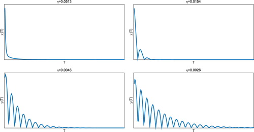
It is easy to show that $\chi \left(T\right)$ is bounded by a decreasing function as the proof of Proposition 5.2 will show. Roughly speaking, the trend of $\chi \left(T\right)$ is to be a decreasing function, where oscillations may occur, and we refer to Figure 1. On the other hand, one can anticipate that the more oscillations of the discrepancy function $\chi \left(T\right)$ occur, the smaller the damping parameter η is. This is an expected result due to the behaviour of damped Hamiltonian systems.

Figure 1. The behaviour of $\chi \left(T\right)$ from (34(34) $\chi \left(T\right):=\parallel Ax\left(T\right)-y^{\delta }\parallel -\tau \delta =0,$(34) ) with different damping parameters η.

5.2. The total energy discrepancy principle

For presenting a newly developed discrepancy principle, we introduce the total energy discrepancy function as follows: (40) ${\chi }_{te}\left(T\right):=\parallel Ax\left(T\right)-y^{\delta }{\parallel }^2+\parallel \dot{x}\left(T\right){\parallel }^2-{\tau }^2{\delta }^2,$(40) where $\tau >{\gamma }_1$ as before.

Proposition 5.2

The function ${\chi }_{te}\left(T\right)$ is continuous and monotonically non-increasing. If $\parallel A{x}_0-y^{\delta }{\parallel }^2+\parallel {\dot{x}}_0{\parallel }^2>{\tau }^2{\delta }^2$, then ${\chi }_{te}\left(T\right)=0$ has a unique solution.

Proof.

The continuity of ${\chi }_{te}\left(T\right)$ is obvious according to Theorem 3.1. The non-growth of ${\chi }_{te}\left(T\right)$ is straight-forward according to ${\dot{\chi }}_{te}=-2\eta \parallel \dot{x}{\parallel }^2$. Furthermore, from (16(16) $\underset{t\to \mathrm{\infty }}{lim}\parallel Ax\left(t\right)-y^{\delta }\parallel \le \delta$(16) ), (17(17) $\underset{t\to \mathrm{\infty }}{lim}\parallel Ax\left(t\right)-y^{\delta }{\parallel }^2+\parallel \dot{x}\left(t\right){\parallel }^2=\underset{x^{\ast }\in \mathcal{X}}{inf}\parallel A{x}^{\ast }-y^{\delta }{\parallel }^2.$(17) ) and the assumption of the proposition, we derive that (41) $\underset{T\to \mathrm{\infty }}{lim}{\chi }_{te}\left(T\right)\le {\delta }^2(1-{\tau }^2)<0,$(41) and that, moreover, ${\chi }_{te}\left(0\right)=\parallel A{x}_0-y^{\delta }{\parallel }^2+\parallel {\dot{x}}_0{\parallel }^2-{\tau }^2{\delta }^2>0$. This implies the existence of roots for ${\chi }_{te}\left(T\right)$.

Finally, let us show that ${\chi }_{te}\left(T\right)$ has a unique solution. We prove this by contradiction. Since ${\chi }_{te}\left(T\right)$ is a non-increasing function, a number $T_0$ exists so that ${\chi }_{te}\left(T\right)=0$ for $T\in [T_0,T_0+\epsilon ]$ with some positive $\epsilon >0$. This means that ${\dot{\chi }}_{te}\left(T\right)=-2\eta \parallel \dot{x}{\parallel }^2\equiv 0$ in $(T_0,T_0+\epsilon )$. Hence, $\ddot{x}\equiv 0$ in $(T_0,T_0+\epsilon )$. Using equation (4(4) $\begin{array}{rl}& \ddot{x}\left(t\right)+\eta \dot{x}\left(t\right)+A^{\ast }Ax\left(t\right)=A^{\ast }{y}^{\delta },\\ & x\left(0\right)=x_0,\dot{x}\left(0\right)={\dot{x}}_0\end{array}$(4) ) we conclude that for all $T>T_0$: $x\left(T\right)\equiv x\left(T_0\right)$. Since ${\chi }_{te}\left(T_0\right)=0$, we obtain that ${\chi }_{te}\left(T\right)\equiv 0$ for $T>T_0$, which implies that $\underset{T\to \mathrm{\infty }}{lim}{\chi }_{te}\left(T\right)=0$. This contradicts the fact in (41(41) $\underset{T\to \mathrm{\infty }}{lim}{\chi }_{te}\left(T\right)\le {\delta }^2(1-{\tau }^2)<0,$(41) ).

Theorem 5.3

A posteriori choice II of the regularization parameter 

Assume that $\parallel A{x}_0-y^{\delta }{\parallel }^2+\parallel {\dot{x}}_0{\parallel }^2>{\tau }^2{\delta }^2$ and a positive number ${\delta }_1$ exists such that for all $\delta \in (0,{\delta }_1]$, the unique root $T^{\ast }$ of ${\chi }_{te}\left(T\right)$ satisfies the inequality $\parallel Ax\left(T^{\ast }\right)-y^{\delta }\parallel \ge {\tau }_1\delta$, where ${\tau }_1>{\gamma }_1$ is a constant, independent of δ. Then, under the source conditions (30(30) $x_0-x^{†}=(A^{\ast }A{)}^p{v}_0\mathrm{with}\parallel v_0\parallel \le \rho .$(30) ) and (31(31) ${\dot{x}}_0=(A^{\ast }A{)}^p{v}_1\mathrm{with}\parallel v_1\parallel \le \rho .$(31) ), for any $\delta \in (0,{\delta }_0]$ and p>0 we have the error estimates (42) $T^{\ast }\le C_0{\rho }^{2/(2p+1)}{\delta }^{-2/(2p+1)},\parallel x\left(T^{\ast }\right)-x^{†}\parallel \le C_1{\delta }^{2p/(2p+1)},$(42) where ${\delta }_0$ is defined in Theorem 5.1, and constants $C_0$ and $C_1$ are the same as in Theorem   5.2.

Proof.

The proof can be done along the lines and using the tools of the proof of Theorem 5.2.

In the simulation Section 7.1, we will computationally show that the assumptions occurring in the above theorem can happen in practice. Empirically, when the value of the initial velocity is not too small ($\parallel {\dot{x}}_0\parallel >0$) or the noise is small enough ($\delta \ll 1$), the additional assumption $\parallel Ax\left(T^{\ast }\right)-y^{\delta }\parallel \ge {\tau }_1\delta$ in Theorem 5.3 always holds.

6. A novel iterative regularization method

Roughly speaking, the second-order evolution equation (4(4) $\begin{array}{rl}& \ddot{x}\left(t\right)+\eta \dot{x}\left(t\right)+A^{\ast }Ax\left(t\right)=A^{\ast }{y}^{\delta },\\ & x\left(0\right)=x_0,\dot{x}\left(0\right)={\dot{x}}_0\end{array}$(4) ) with an appropriate numerical discretization scheme for the artificial time variable yields a concrete second-order iterative method. Just as with the Runge–Kutta integrators [6] or the exponential integrators [26] for solving first-order equations, the damped symplectic integrators are extremely attractive for solving second-order equations, since the schemes are closely related to the canonical transformations [27], and the trajectories of the discretized second flow are usually more stable.

The simplest discretization scheme should be the Euler method. Denote by $v=\dot{x}$, and consider the following Euler iteration: (43) $\begin{array}{rl}{x}^{k+1}& =x^k+\mathrm{\Delta }{t}_k{v}^k,\\ v^{k+1}& =v^k+\mathrm{\Delta }{t}_k\left(A^{\ast }\right(y^{\delta }-A{x}^{k+1})-\eta v^k),\\ x^0& =x_0,v^0={\dot{x}}_0.\end{array}$(43) By elementary calculations, scheme (43(43) $\begin{array}{rl}{x}^{k+1}& =x^k+\mathrm{\Delta }{t}_k{v}^k,\\ v^{k+1}& =v^k+\mathrm{\Delta }{t}_k\left(A^{\ast }\right(y^{\delta }-A{x}^{k+1})-\eta v^k),\\ x^0& =x_0,v^0={\dot{x}}_0.\end{array}$(43) ) expresses the form of following three-term semi-iterative method: (44) $x^{k+1}=x^k+{\mu }_k(x^k-x^{k-1})+{\omega }_k{A}^{\ast }(y^{\delta }-A{x}^k)$(44) with a specially defined parameters ${\omega }_k=\mathrm{\Delta }{t}_k$ and ${\mu }_k=1-\mathrm{\Delta }{t}_k\eta$. It is well known that the semi-iterative method (44(44) $x^{k+1}=x^k+{\mu }_k(x^k-x^{k-1})+{\omega }_k{A}^{\ast }(y^{\delta }-A{x}^k)$(44) ), equipped with an appropriate stopping rule, yields order optimal regularization method with (asymptotically) much fewer iterations than the classical Landweber iteration [2, Section 6.2].

In this paper, we develop a new iterative regularization method based on the Störmer–Verlet method, which also belongs to the family of symplectic integrators and takes the form (45) $\begin{array}{rl}{v}^{k+1/2}& =v^k+\frac{\mathrm{\Delta }t}{2}\left(A^{\ast }\right(y^{\delta }-A{x}^k)-\eta v^{k+1/2}),\\ x^{k+1}& =x^k+\mathrm{\Delta }t{v}^{k+1/2},\\ v^{k+1}& =v^{k+1/2}+\frac{\mathrm{\Delta }t}{2}\left(A^{\ast }\right(y^{\delta }-A{x}^{k+1})-\eta v^{k+1/2}),\\ x^0& =x_0,v^0={\dot{x}}_0.\end{array}$(45)

Proposition 6.1

For any fixed damping parameter η, if the step size is chosen by (46) $\mathrm{\Delta }t\le min(\sqrt{2}/\parallel A\parallel ,2/\eta ),$(46) then, the scheme (45(45) $\begin{array}{rl}{v}^{k+1/2}& =v^k+\frac{\mathrm{\Delta }t}{2}\left(A^{\ast }\right(y^{\delta }-A{x}^k)-\eta v^{k+1/2}),\\ x^{k+1}& =x^k+\mathrm{\Delta }t{v}^{k+1/2},\\ v^{k+1}& =v^{k+1/2}+\frac{\mathrm{\Delta }t}{2}\left(A^{\ast }\right(y^{\delta }-A{x}^{k+1})-\eta v^{k+1/2}),\\ x^0& =x_0,v^0={\dot{x}}_0.\end{array}$(45) ) is convergent. Consequently, for any fixed T, there exists a pair of parameters $(k,\mathrm{\Delta }t),$ satisfying $k\mathrm{\Delta }t=T$ and the condition (46(46) $\mathrm{\Delta }t\le min(\sqrt{2}/\parallel A\parallel ,2/\eta ),$(46) ), such that $x^k=x\left(T\right)+\mathcal{O}\left(\mathrm{\Delta }{t}^2\right)$ as $\mathrm{\Delta }t\to 0$. Here $x^k$ and $x(\cdot )$ are solutions to (45(45) $\begin{array}{rl}{v}^{k+1/2}& =v^k+\frac{\mathrm{\Delta }t}{2}\left(A^{\ast }\right(y^{\delta }-A{x}^k)-\eta v^{k+1/2}),\\ x^{k+1}& =x^k+\mathrm{\Delta }t{v}^{k+1/2},\\ v^{k+1}& =v^{k+1/2}+\frac{\mathrm{\Delta }t}{2}\left(A^{\ast }\right(y^{\delta }-A{x}^{k+1})-\eta v^{k+1/2}),\\ x^0& =x_0,v^0={\dot{x}}_0.\end{array}$(45) ) and (4(4) $\begin{array}{rl}& \ddot{x}\left(t\right)+\eta \dot{x}\left(t\right)+A^{\ast }Ax\left(t\right)=A^{\ast }{y}^{\delta },\\ & x\left(0\right)=x_0,\dot{x}\left(0\right)={\dot{x}}_0\end{array}$(4) ), respectively.

Proof.

Denote by $\mathbf{z}=(x,v{)}^{\mathrm{T}},$ and rewritten (45(45) $\begin{array}{rl}{v}^{k+1/2}& =v^k+\frac{\mathrm{\Delta }t}{2}\left(A^{\ast }\right(y^{\delta }-A{x}^k)-\eta v^{k+1/2}),\\ x^{k+1}& =x^k+\mathrm{\Delta }t{v}^{k+1/2},\\ v^{k+1}& =v^{k+1/2}+\frac{\mathrm{\Delta }t}{2}\left(A^{\ast }\right(y^{\delta }-A{x}^{k+1})-\eta v^{k+1/2}),\\ x^0& =x_0,v^0={\dot{x}}_0.\end{array}$(45) ) as (47) ${\mathbf{z}}^{k+1}=B{\mathbf{z}}^k+\frac{\mathrm{\Delta }t}{2+\mathrm{\Delta }t\eta }\mathbf{b},$(47) where $\mathbf{b}=[\mathrm{\Delta }t;2I-(\mathrm{\Delta }{t}^2/2\left)A^{\ast }A\right]A^{\ast }{y}_{\delta }$ and $B=\left[\begin{array}{cc}I-\frac{\mathrm{\Delta }{t}^2}{2+\mathrm{\Delta }t\eta }{A}^{\ast }A& \frac{2\mathrm{\Delta }t}{2+\mathrm{\Delta }t\eta }I\\ -\frac{\mathrm{\Delta }t}{2(2+\mathrm{\Delta }t\eta )}(4I-\mathrm{\Delta }{t}^2{A}^{\ast }A)A^{\ast }A& \frac{2-\mathrm{\Delta }t\eta }{2+\mathrm{\Delta }t\eta }I-\frac{\mathrm{\Delta }{t}^2}{2+\mathrm{\Delta }t\eta }{A}^{\ast }A\end{array}\right].$

By Taylor's theorem and the finite difference formula, it is not difficult to show the consistency of the scheme (45(45) $\begin{array}{rl}{v}^{k+1/2}& =v^k+\frac{\mathrm{\Delta }t}{2}\left(A^{\ast }\right(y^{\delta }-A{x}^k)-\eta v^{k+1/2}),\\ x^{k+1}& =x^k+\mathrm{\Delta }t{v}^{k+1/2},\\ v^{k+1}& =v^{k+1/2}+\frac{\mathrm{\Delta }t}{2}\left(A^{\ast }\right(y^{\delta }-A{x}^{k+1})-\eta v^{k+1/2}),\\ x^0& =x_0,v^0={\dot{x}}_0.\end{array}$(45) ). It is well known that boundedness implies the convergence of consistent schemes for any problem [28], hence, it suffices to show the boundedness of the scheme (45(45) $\begin{array}{rl}{v}^{k+1/2}& =v^k+\frac{\mathrm{\Delta }t}{2}\left(A^{\ast }\right(y^{\delta }-A{x}^k)-\eta v^{k+1/2}),\\ x^{k+1}& =x^k+\mathrm{\Delta }t{v}^{k+1/2},\\ v^{k+1}& =v^{k+1/2}+\frac{\mathrm{\Delta }t}{2}\left(A^{\ast }\right(y^{\delta }-A{x}^{k+1})-\eta v^{k+1/2}),\\ x^0& =x_0,v^0={\dot{x}}_0.\end{array}$(45) ). The asymptotical behaviour $x^k=x\left(T\right)+\mathcal{O}\left(\mathrm{\Delta }{t}^2\right)$ follows from the convergence result and the second order of the Störmer–Verlet method. Furthermore, a sufficient condition for the boundedness of the iterative algorithm (45(45) $\begin{array}{rl}{v}^{k+1/2}& =v^k+\frac{\mathrm{\Delta }t}{2}\left(A^{\ast }\right(y^{\delta }-A{x}^k)-\eta v^{k+1/2}),\\ x^{k+1}& =x^k+\mathrm{\Delta }t{v}^{k+1/2},\\ v^{k+1}& =v^{k+1/2}+\frac{\mathrm{\Delta }t}{2}\left(A^{\ast }\right(y^{\delta }-A{x}^{k+1})-\eta v^{k+1/2}),\\ x^0& =x_0,v^0={\dot{x}}_0.\end{array}$(45) ) is that the operator B is non-expansive. Hence, it is necessary to prove that $\parallel B{\parallel }_2\le 1$.

Using the singular value decomposition, we have $A^{\ast }A=\mathrm{\Phi \Lambda }{\mathrm{\Phi }}^{\mathrm{T}}$, where Φ is a unitary matrix and $\mathrm{\Lambda }=\mathrm{diag}\left({\lambda }_i\right)$, where ${\lambda }_i\ge 0,i=1,\dots ,n$.

By the elementary calculations, we obtain that the eigenvalues of B equal (48) ${\mu }_i^{\pm }=\frac{1}{2+\mathrm{\Delta }t\eta }\left\{\right(2-\mathrm{\Delta }{t}^2{\lambda }_i)\pm \sqrt{(2-\mathrm{\Delta }{t}^2{\lambda }_i{)}^2-(4-\mathrm{\Delta }{t}^2{\eta }^2)}\},i=1,\dots ,n.$(48)

Denote by $i_{\ast }$ the index of ${\lambda }_{i_{\ast }}$, corresponding to the maximal absolute value of ${\mu }_i^{\pm }$, i.e. $|{\mu }_{max}|=\frac{1}{2+\mathrm{\Delta }t\eta }\underset{\pm }{max}\left|(2-\mathrm{\Delta }{t}^2{\lambda }_{i_{\ast }})\pm \sqrt{(2-\mathrm{\Delta }{t}^2{\lambda }_{i_{\ast }}{)}^2-(4-\mathrm{\Delta }{t}^2{\eta }^2)}\right|.$

There are three possible cases here: the overdamped case ($(2-\mathrm{\Delta }{t}^2{\lambda }_{i_{\ast }}{)}^2>4-\mathrm{\Delta }{t}^2{\eta }^2$), the underdamped case ($(2-\mathrm{\Delta }{t}^2{\lambda }_{i_{\ast }}{)}^2<4-\mathrm{\Delta }{t}^2{\eta }^2$), and the critical damping case ($(2-\mathrm{\Delta }{t}^2{\lambda }_{i_{\ast }}{)}^2=4-\mathrm{\Delta }{t}^2{\eta }^2$).

Let us consider these cases, respectively. For the chosen time step size $\mathrm{\Delta }t$ in (46(46) $\mathrm{\Delta }t\le min(\sqrt{2}/\parallel A\parallel ,2/\eta ),$(46) ), we have $2-\mathrm{\Delta }{t}^2{\lambda }_{i_{\ast }}\ge 0$. Therefore, for the overdamped case, $|{\mu }_{max}|=\frac{1}{2+\mathrm{\Delta }t\eta }\left\{\right(2-\mathrm{\Delta }{t}^2{\lambda }_{i_{\ast }})+\sqrt{(2-\mathrm{\Delta }{t}^2{\lambda }_{i_{\ast }}{)}^2-(4-\mathrm{\Delta }{t}^2{\eta }^2)}\}.$ Define $2-\mathrm{\Delta }{t}^2{\lambda }_{i_{\ast }}=a\sqrt{4-\mathrm{\Delta }{t}^2{\eta }^2}$ with a>1 (by the condition (46(46) $\mathrm{\Delta }t\le min(\sqrt{2}/\parallel A\parallel ,2/\eta ),$(46) ), it holds that $4-\mathrm{\Delta }{t}^2{\eta }^2\ge 0$), and we have (49) $|{\mu }_{max}|=\frac{(a+\sqrt{a^2-1})\sqrt{4-\mathrm{\Delta }{t}^2{\eta }^2}}{2+\mathrm{\Delta }t\eta }=\frac{(a+\sqrt{a^2-1})(2-\mathrm{\Delta }{t}^2{\lambda }_{i_{\ast }})}{a(2+\mathrm{\Delta }t\eta )}.$(49) Note that (50) $\mathrm{\Delta }t\eta =\sqrt{4-{\left(\frac{2-\mathrm{\Delta }{t}^2{\lambda }_{i_{\ast }}}{a}\right)}^2}.$(50) Combine (49(49) $|{\mu }_{max}|=\frac{(a+\sqrt{a^2-1})\sqrt{4-\mathrm{\Delta }{t}^2{\eta }^2}}{2+\mathrm{\Delta }t\eta }=\frac{(a+\sqrt{a^2-1})(2-\mathrm{\Delta }{t}^2{\lambda }_{i_{\ast }})}{a(2+\mathrm{\Delta }t\eta )}.$(49) ) and (50(50) $\mathrm{\Delta }t\eta =\sqrt{4-{\left(\frac{2-\mathrm{\Delta }{t}^2{\lambda }_{i_{\ast }}}{a}\right)}^2}.$(50) ) to obtain $|{\mu }_{max}|=\frac{(a+\sqrt{a^2-1})(2-\mathrm{\Delta }{t}^2{\lambda }_{i_{\ast }})}{2a+\sqrt{4a^2-(2-\mathrm{\Delta }{t}^2{\lambda }_{i_{\ast }}{)}^2}}=\frac{(a+\sqrt{a^2-1})(1-{\displaystyle \frac{\mathrm{\Delta }{t}^2{\lambda }_{i_{\ast }}}{2}})}{a+\sqrt{a^2-{\left(1-{\displaystyle \frac{\mathrm{\Delta }{t}^2{\lambda }_{i_{\ast }}}{2}}\right)}^2}}\le 1-\frac{\mathrm{\Delta }{t}^2{\lambda }_{i_{\ast }}}{2}\le 1.$ Now, consider the underdamped case. In this case, the complex eigenvalue ${\mu }_{max}$ satisfies $|{\mu }_{max}{|}^2=\frac{1}{(2+\mathrm{\Delta }t\eta {)}^2}\left\{\right(2-\mathrm{\Delta }{t}^2{\lambda }_{i_{\ast }}{)}^2+\left[\right(4-\mathrm{\Delta }{t}^2{\eta }^2)-(2-\mathrm{\Delta }{t}^2{\lambda }_{i_{\ast }}{)}^2\left]\right\},$ which implies that $|{\mu }_{max}{|}^2=\frac{4-\mathrm{\Delta }{t}^2{\eta }^2}{(2+\mathrm{\Delta }t\eta {)}^2}=\frac{2-\mathrm{\Delta }t\eta }{2+\mathrm{\Delta }t\eta }<1.$ Finally, consider the critical damping case. Similarly, we have $|{\mu }_{max}|=\sqrt{(2-\mathrm{\Delta }t\eta )/(2+\mathrm{\Delta }t\eta )}<1$, which yields the desired result.

At the end of this second, we show the convergence rate of the scheme (45(45) $\begin{array}{rl}{v}^{k+1/2}& =v^k+\frac{\mathrm{\Delta }t}{2}\left(A^{\ast }\right(y^{\delta }-A{x}^k)-\eta v^{k+1/2}),\\ x^{k+1}& =x^k+\mathrm{\Delta }t{v}^{k+1/2},\\ v^{k+1}& =v^{k+1/2}+\frac{\mathrm{\Delta }t}{2}\left(A^{\ast }\right(y^{\delta }-A{x}^{k+1})-\eta v^{k+1/2}),\\ x^0& =x_0,v^0={\dot{x}}_0.\end{array}$(45) ).

Theorem 6.1

Under the assumptions of Theorem 5.2 or 5.3, if the time step size is chosen by $\mathrm{\Delta }t=C_t{\delta }^{p/(2p+1)},$ then for any $\delta \in (0,{\delta }_s]$ and p>0 we have the convergence rate (51) $\parallel x^{k^{\ast }}-x^{†}\parallel =\mathcal{O}\left({\delta }^{2p/(2p+1)}\right),$(51) where $k^{\ast }=T^{\ast }/\mathrm{\Delta }t$ , ${\delta }_s=min\left\{\right(\sqrt{2}/C_t{)}^{2+1/p}\parallel A{\parallel }^{-2-1/p},(2/C_t{)}^{2+1/p}{\eta }^{-2-1/p},{\delta }_0\}$, $C_t=\left(T^{\ast }/{\delta }^{p/(2p+1)}\right)/\lfloor T^{\ast }/{\delta }^{p/(2p+1)}\rfloor$, and $T^{\ast }$ is the root of (34(34) $\chi \left(T\right):=\parallel Ax\left(T\right)-y^{\delta }\parallel -\tau \delta =0,$(34) ) or (40(40) ${\chi }_{te}\left(T\right):=\parallel Ax\left(T\right)-y^{\delta }{\parallel }^2+\parallel \dot{x}\left(T\right){\parallel }^2-{\tau }^2{\delta }^2,$(40) ). Here, $\lfloor \cdot \rfloor$ denotes the standard floor function and ${\delta }_0$ is defined in Theorem 5.1.

Proof.

It follows from Proposition 6.1 that the choice $\mathrm{\Delta }t=C_t{\delta }^{p/(2p+1)}$ yields $\parallel x^{k^{\ast }}-x\left(T^{\ast }\right)\parallel \le C{\delta }^{2p/(2p+1)}$ with some constant C for all $\delta \in (0,{\delta }_s]$.

Combine the above inequality and the results in Theorems 5.2 and 5.3 to obtain $\parallel x^{k^{\ast }}-x^{†}\parallel \le \parallel x^k-x\left(T^{\ast }\right)\parallel +\parallel x\left(T^{\ast }\right)-x^{†}\parallel \le C_r{\delta }^{2p/(2p+1)}$ for some constant $C_r$. This gives the estimate (51(51) $\parallel x^{k^{\ast }}-x^{†}\parallel =\mathcal{O}\left({\delta }^{2p/(2p+1)}\right),$(51) ).

7. Numerical simulations

In this section, we present some numerical results for the following integral equation: (52) $Ax\left(s\right):={\int }_0^{1}K(s,t)x\left(t\right)\mathrm{d}t=y\left(s\right),K(s,t)=s(1-t){\chi }_{s\le t}+t(1-s){\chi }_{s>t}.$(52) If we choose $\mathcal{X}=\mathcal{Y}=L^2[0,1]$, the operator A is compact, selfadjoint and injective. It is well known that the integral equation (52(52) $Ax\left(s\right):={\int }_0^{1}K(s,t)x\left(t\right)\mathrm{d}t=y\left(s\right),K(s,t)=s(1-t){\chi }_{s\le t}+t(1-s){\chi }_{s>t}.$(52) ) has a solution $x=-y^{″}$ if $y\in H^2[0,1]\cap H_0^1[0,1]$. Moreover, the operator A has the eigensystem $A{u}_j={\sigma }_j{u}_j$, where ${\sigma }_j=(j\pi {)}^{-2}$ and $u_j\left(t\right)=\sqrt{2}\sin \left(j\pi t\right)$. Furthermore, using the interpolation theory (see e.g. [29]) it is not difficult to show that for $4p-1/2\notin \mathbf{N}$ $R\left(\right(A^{\ast }A{)}^p)=\{x\in H^{4p}[0,1]:x^{2l}\left(0\right)=x^{2l}\left(1\right)=0,l=0,1,\dots ,\lfloor 2p-1/4\rfloor \}.$ In general, a regularization procedure becomes numerically feasible only after an appropriate discretization. Here, we apply the linear finite elements to solve (52(52) $Ax\left(s\right):={\int }_0^{1}K(s,t)x\left(t\right)\mathrm{d}t=y\left(s\right),K(s,t)=s(1-t){\chi }_{s\le t}+t(1-s){\chi }_{s>t}.$(52) ). Let ${\mathcal{Y}}_n$ be the finite element space of piecewise linear functions on a uniform grid with step size $1/(n-1)$. Denote by $P_n$ the orthogonal projection operator acting from $\mathcal{Y}$ into ${\mathcal{Y}}_n$. Define $A_n:=P_{n}A$ and ${\mathcal{X}}_n:=A_n^{\ast }{\mathcal{Y}}_n$. Let $\{{\phi }_j{\}}_{j=1}^n$ be a basis of the finite element space ${\mathcal{Y}}_n$, then, instead of the original problem (52(52) $Ax\left(s\right):={\int }_0^{1}K(s,t)x\left(t\right)\mathrm{d}t=y\left(s\right),K(s,t)=s(1-t){\chi }_{s\le t}+t(1-s){\chi }_{s>t}.$(52) ), we solve the following system of linear equations: (53) $A_n{x}_n=y_n,$(53) where $[A_n{]}_{ij}={\int }_0^1({\int }_0^{1}k(s,t){\phi }_i\left(s\right)\mathrm{d}s\left){\phi }_j\right(t)\mathrm{d}t$ and $[y_n{]}_j={\int }_0^{1}y(t\left){\phi }_j\right(t)\mathrm{d}t$.

As shown in [2], the finite dimensional projection error ${ϵ}_n:=\parallel (I-P_n)A\parallel$ plays an important role in the convergence rates analysis. For the compact operator A, ${ϵ}_n\to 0$ as $n\to \mathrm{\infty }$. Moreover, if the noise level $\delta \to 0$ slowly enough as $n\to \mathrm{\infty }$, the quality ${ϵ}_n$ has no influence and we obtain the same convergence rates as in Theorems 5.2 and 5.3.

Uniformly distributed noises with the magnitude ${\delta }^{\prime }$ are added to the discretized exact right-hand side: (54) $[y_n^{\delta }{]}_j:=[1+{\delta }^{\prime }\cdot \left(2\mathrm{Rand}\right(x)-1)]\cdot [y_n{]}_j,j=1,\dots ,n,$(54) where $\mathrm{Rand}\left(x\right)$ returns a pseudo-random value drawn from a uniform distribution on [0,1]. The noise level of measurement data is calculated by $\delta =\parallel y_n^{\delta }-y_n{\parallel }_2$, where $\parallel \cdot {\parallel }_2$ denotes the standard vector norm in ${\mathbf{R}}^n$.

To assess the accuracy of the approximate solutions, we define the $L^2$-norm relative error for an approximate solution $x_n^{k^{\ast }}$ ($k^{\ast }=\lfloor T^{\ast }/\mathrm{\Delta }t\rfloor$): $\mathrm{L}2\mathrm{Err}:=\parallel x_n^{k^{\ast }}-x^{†}{\parallel }_{L^2[0,1]}/\parallel x^{†}{\parallel }_{L^2[0,1]},$ where $x^{†}$ is the exact solution to the corresponding model problem.

7.1. Influence of parameters

The purpose of this subsection is to explore the dependence of the solution accuracy and the convergence rate on the initial data $(x_0,{\dot{x}}_0)$, damping parameter η and the discrepancy functions χ and ${\chi }_{te}$, and thus to give a guide on the choices of them in practice.

In this subsection, we solve integral equation (52(52) $Ax\left(s\right):={\int }_0^{1}K(s,t)x\left(t\right)\mathrm{d}t=y\left(s\right),K(s,t)=s(1-t){\chi }_{s\le t}+t(1-s){\chi }_{s>t}.$(52) ) with the exact right-hand side $y=s(1-s)$. Then, the exact solution $x^{†}=2$, and $x^{†}\in R\left(\right(A^{\ast }A{)}^p)$ for all $p<1/8$. Denote by ‘DP’ and ‘TEDP’ the newly developed iterative scheme (45(45) $\begin{array}{rl}{v}^{k+1/2}& =v^k+\frac{\mathrm{\Delta }t}{2}\left(A^{\ast }\right(y^{\delta }-A{x}^k)-\eta v^{k+1/2}),\\ x^{k+1}& =x^k+\mathrm{\Delta }t{v}^{k+1/2},\\ v^{k+1}& =v^{k+1/2}+\frac{\mathrm{\Delta }t}{2}\left(A^{\ast }\right(y^{\delta }-A{x}^{k+1})-\eta v^{k+1/2}),\\ x^0& =x_0,v^0={\dot{x}}_0.\end{array}$(45) ) equipped with the Morozov's conventional discrepancy function $\chi \left(T\right)$ and the total energy discrepancy functions ${\chi }_{te}\left(T\right)$, respectively.

The results about the influence of the solution accuracy (L2Err) and the convergence rate (iteration numbers $k^{\ast }\left(\delta \right)$) on the initial data $(x_0,{\dot{x}}_0)$ are given in Tables 1 and 2, respectively. As we can see, both the initial data $x_0$ and ${\dot{x}}_0$ influence the solution accuracy as well as the convergence rate. Moreover, when the value of the damping parameter is not too small (see Tables 2 and  3) the results (both solution accuracy and convergence rate) by the methods ‘DP’ and ‘TEDP’ almost coincide with each other. This result verifies the rationality of the assumption in Theorem 5.3.

Table 1. The dependence of the solution accuracy and the convergence rate on the initial data $x_0$. $\mathrm{\Delta }t=19.4946,\eta =2.5648\times {10}^{-4},{\dot{x}}_0=0,\tau =2,p=0.1125$.

		DP		TEDP
δ (${\delta }^{\prime }$)	$x_0$	$k^{\ast }\left(\delta \right)$	L2Err	$k^{\ast }\left(\delta \right)$	L2Err
7.1191e−04 (1e−03)	0	1295	0.2214	2033	0.2894
7.1337e−04 (1e−03)	$-1$	1354	0.2284	2210	0.2825
7.0838e−04 (1e−03)	1	1108	0.1965	1777	0.1414
7.1602e−05 (1e−04)	0	2397	0.0688	2958	0.0653
8.0523e−05 (1e−04)	$-1$	2525	0.0983	3076	0.0920
7.8903e−05 (1e−04)	1	1600	0.0449	2643	0.0431

Table 2. The dependence of the solution accuracy and the convergence rate on the initial data ${\dot{x}}_0$. $\mathrm{\Delta }t=19.4946,\eta =0.0154,x_0=1,\tau =2,p=0.1125$.

		DP		TEDP
δ (${\delta }^{\prime }$)	${\dot{x}}_0$	$k^{\ast }\left(\delta \right)$	L2Err	$k^{\ast }\left(\delta \right)$	L2Err
6.3541e−04 (1e−03)	0	155	0.1062	156	0.1061
7.3673e−04 (1e−03)	$-0.01$	374	0.1576	376	0.1574
7.1484e−04 (1e−03)	0.01	39	0.0443	39	0.0443
8.0763e−05 (1e−04)	0	4559	0.0675	4561	0.0675
7.3174e−05 (1e−04)	$-0.01$	12466	0.0953	12467	0.0953
7.6200e−05 (1e−04)	0.01	982	0.0293	983	0.0293

Table 3. The dependence of the solution accuracy and the convergence rate on the damping parameter η. $\mathrm{\Delta }t=19.4946,x_0=1,{\dot{x}}_0=0,\tau =2,p=0.1125$.

		DP		TEDP
δ (${\delta }^{\prime }$)	η	$k^{\ast }\left(\delta \right)$	L2Err	$k^{\ast }\left(\delta \right)$	L2Err
8.7715e−04 (1e−03)	2.5648e−05	6943	0.8319	17393	0.7744
7.3673e−04 (1e−03)	2.5648e−04	1108	0.1310	1728	0.1080
7.1484e−04 (1e−03)	2.5648e−03	124	0.0901	183	0.0870
8.1011e−05 (1e−04)	2.5648e−02	205	0.1101	206	0.1100
7.3174e−05 (1e−04)	0.0513	398	0.1108	398	0.1108
7.2721e−05 (1e−04)	0.1026 ($=2/\mathrm{\Delta }t$)	848	0.1096	848	0.1096

In Table 3, we displayed the numerical results with different value of damping parameters η. With the appropriate choice of the damping parameter, say $\eta =2.5648\times {10}^{-3}$ in our example, the SOAR not only gives the most accurate result but exhibits an acceleration effect. The critical value of the damping parameter, say $\eta =2/\mathrm{\Delta }t$, also provides an accurate result. But it requires a few more steps. The influence of the damping parameter on the residual functional can be found in Figure 1. It shows that at the same time point, the larger the damping parameter, the smaller the residual norm functional.

7.2. Comparison with other methods

In order to demonstrate the advantages of our algorithm over the traditional approaches, we solve the same problems by four famous iterative regularization methods – the Landweber method, the Nesterov's method, the ν-method and the conjugate gradient method for the normal equation (CGNE, cf., e.g. [30]). The Landweber method is given in (2(2) $x_{k+1}=x_k+\mathrm{\Delta }t{A}^{\ast }(y^{\delta }-A{x}_k),\mathrm{\Delta }t\in (0,2/\parallel A{\parallel }^2),$(2) ), while Nesterov's method is defined as [31] (55) $\begin{array}{rl}{z}^k& =x^k+\frac{k-1}{k+\alpha -1}(x^k-x^{k-1}),\\ x^{k+1}& =z^k+\mathrm{\Delta }t{A}^{\ast }(y^{\delta }-A{z}^k),\end{array}$(55) where $\alpha >3$ (we choose $\alpha =3.1$ in our simulations). Moreover, we select the Chebyshev method as our special ν-method, i.e. $\nu =1/2$ [2, Section 6.3]. For all of four traditional iterative regularization methods, we use the Morozov's conventional discrepancy principle as the stopping rule.

We consider the following two different right-hand sides for the integral equation (52(52) $Ax\left(s\right):={\int }_0^{1}K(s,t)x\left(t\right)\mathrm{d}t=y\left(s\right),K(s,t)=s(1-t){\chi }_{s\le t}+t(1-s){\chi }_{s>t}.$(52) ).

• Example 1: $y\left(s\right)=s(1-s)$. Then, $x^{†}=2$, and $x^{†}\in R\left(\right(A^{\ast }A{)}^p)$ for all $p<1/8$. This example uses the discretization size n=400. Other parameters are $\mathrm{\Delta }t=19.4946,\eta =2.5648\times {10}^{-4},x_0=1,{\dot{x}}_0=0,\tau =2,p=0.1125$.

• Example 2: $y\left(s\right)=s^4(1-s{)}^3$. Then, $x^{†}=-6t^2(1-t)(2-8t+7t^2)$, and $x^{†}\in R\left(\right(A^{\ast }A{)}^p)$ for all $p<5/8$. This example uses the discretization size n=400. Other parameters are $\mathrm{\Delta }t=19.4946,\eta =0.0051,x_0=0,{\dot{x}}_0=0,\tau =2,p=0.5625$.

The results of the simulation are presented in Table 4, where we can conclude that, in general, the SOAR need less iteration and CPU time, and offers a more accurate regularization solution. Moreover, with respect to the Morozov's conventional discrepancy principle, the newly developed total energy discrepancy principle provides more accurate results in most cases. Concerning the number of iterations, the CGNE method performed much better than all of the other methods. However, the accuracy of the CGNE method is much worse than other methods (including DP and TEDP), since the step size of CGNE is too large to capture the optimal point and the semi-convergence effect disturbs the iteration rather early. Note that we set a maximal iteration number $k_{max}=400,000$ in all of our simulations.

Table 4. Comparisons with the Landweber method, the Nesterov's method, the Chebyshev method, and the CGNE method.

	DP			TEDP			Landweber
δ	$k^{\ast }\left(\delta \right)$	CPU (s)	L2Err	$k^{\ast }\left(\delta \right)$	CPU (s)	L2Err	$k^{\ast }\left(\delta \right)$	CPU (s)	L2Err
Example 1
1.0400e−2	70	0.2023	0.1494	70	0.1995	0.1494	20438	52.6428	0.2639
1.0380e−3	2872	8.9239	0.0945	2871	1.9105	0.0945	$k_{max}$	1.6899e3	0.1807
1.0445e−4	56246	177.3387	0.0597	56246	177.9603	0.0473	$k_{max}$	1.8048e3	0.1807
Example 2
1.0761e−2	15	0.0554	0.3676	25	0.0753	0.1987	1457	6.3672	0.7032
1.0703e−3	93	0.2488	0.0637	132	0.3567	0.0581	23790	67.6082	0.1767
1.1006e−4	453	1.4931	0.0195	531	1.8000	0.0184	187188	679.8274	0.0509
	Nesterov			Chebyshev			CGNE
δ	$k^{\ast }\left(\delta \right)$	CPU (s)	L2Err	$k^{\ast }\left(\delta \right)$	CPU (s)	L2Err	$k^{\ast }\left(\delta \right)$	CPU (s)	L2Err
Example 1
1.0400e−2	419	1.1384	0.2590	264	0.7378	0.2553	6	0.0351	0.2213
1.0380e−3	2813	8.5986	0.1600	2229	7.6512	0.1496	18	0.0904	0.1383
1.0445e−4	16642	60.1179	0.1025	17443	52.2056	0.0897	39	0.2013	0.0894
Example 2
1.0761e−2	102	0.3018	0.7043	62	0.1768	0.7102	6	0.0148	0.4835
1.0703e−3	416	1.1732	0.1676	415	1.1908	0.1190	12	0.0261	0.1514
1.1006e−4	1805	6.0793	0.0280	2226	7.6967	0.0196	15	0.0309	0.0447

8. Conclusion and outlook

In this paper, we have investigated the method of SOAR for solving the ill-posed linear inverse problem Ax=y with the compact operator A mapping between infinite dimensional Hilbert spaces. Instead of y, we are given noisy data $y^{\delta }$ obeying the inequality $\parallel y^{\delta }-y\parallel \le \delta$. We have shown regularization properties for the dynamical solution of the second-order equation (4(4) $\begin{array}{rl}& \ddot{x}\left(t\right)+\eta \dot{x}\left(t\right)+A^{\ast }Ax\left(t\right)=A^{\ast }{y}^{\delta },\\ & x\left(0\right)=x_0,\dot{x}\left(0\right)={\dot{x}}_0\end{array}$(4) ). Moreover, by using Morozov's conventional discrepancy principle on the one hand and a newly developed total energy discrepancy principle on the other hand, we have proven the order optimality of SOAR. Furthermore, based on the framework of SOAR, by using the Störmer–Verlet method, we have derived a novel iterative regularization algorithm. The convergence property of the proposed numerical algorithm is proven as well. Numerical experiments in Section 7 show that, in comparison with conventional iterative regularization methods, SOAR is a faster regularization method for solving linear inverse problems with high levels of accuracy.

Various numerical results show that the damping parameter η in the second-order equation (4(4) $\begin{array}{rl}& \ddot{x}\left(t\right)+\eta \dot{x}\left(t\right)+A^{\ast }Ax\left(t\right)=A^{\ast }{y}^{\delta },\\ & x\left(0\right)=x_0,\dot{x}\left(0\right)={\dot{x}}_0\end{array}$(4) ) plays a prominent role in regularization and acceleration. Therefore, how to choose an optimal damping parameter should be studied in the future. Moreover, using the results of the nonlinear Landweber iteration, it will be possible to develop a theory of SOAR for wide classes of nonlinear ill-posed problems. Furthermore, it could be very interesting to investigate the case with the dynamical damping parameter $\eta =\eta \left(t\right)$. For instance, the second-order equation (4(4) $\begin{array}{rl}& \ddot{x}\left(t\right)+\eta \dot{x}\left(t\right)+A^{\ast }Ax\left(t\right)=A^{\ast }{y}^{\delta },\\ & x\left(0\right)=x_0,\dot{x}\left(0\right)={\dot{x}}_0\end{array}$(4) ) with $\eta =r/t$ ($r\ge 3$) presents the continuous version of Nesterov's scheme [32], and the discretization of (4(4) $\begin{array}{rl}& \ddot{x}\left(t\right)+\eta \dot{x}\left(t\right)+A^{\ast }Ax\left(t\right)=A^{\ast }{y}^{\delta },\\ & x\left(0\right)=x_0,\dot{x}\left(0\right)={\dot{x}}_0\end{array}$(4) ) with $\begin{array}{rl}{\eta }_k& =\frac{(k+2\nu -1)(2k+4\nu -1)(2k+2\nu -3)-(k-1)(2k-3)(3k+3\nu -1)}{4(2k+2\nu -3)(2k+2\nu -1)(k+\nu -1)},\\ \mathrm{\Delta }{t}_k& =4\frac{(2k+2\nu -1)(k+\nu -1)}{(k+2\nu -1)(2k+4\nu -1)},\end{array}$ yields the well-known ν-methods [2, Section 6.3]. Even in the linear case (1(1) $Ax=y,$(1) ), to the best of our knowledge, it is not quite clear whether Nesterov's approach equipped with a posteriori choice of the regularization parameter is an accelerated regularization method for solving ill-posed inverse problems. In our opinion, however, the SOAR can be a candidate for the systematic analysis of general second-order regularization methods.

Disclosure statement

No potential conflict of interest was reported by the authors.

ORCID

Y. Zhang  http://orcid.org/0000-0003-4023-6352

Additional information

Funding

The work of Y. Zhang is supported by the Alexander von Humboldt-Stiftung through a postdoctoral researcher fellowship, and the work of B. Hofmann is supported by the Deutsche Forschungsgemeinschaft [DFG-grant HO 1454/12-1].

Appendix 1. Proofs in Section 3

A.1. Proof of Lemma 3.1

Define the Lyapunov function of (4(4) $\begin{array}{rl}& \ddot{x}\left(t\right)+\eta \dot{x}\left(t\right)+A^{\ast }Ax\left(t\right)=A^{\ast }{y}^{\delta },\\ & x\left(0\right)=x_0,\dot{x}\left(0\right)={\dot{x}}_0\end{array}$(4) ) by $\mathcal{E}\left(T\right)=\parallel Ax\left(T\right)-y^{\delta }{\parallel }^2+\parallel \dot{x}\left(T\right){\parallel }^2$. It is not difficult to show that (A1) $\dot{\mathcal{E}}\left(t\right)=-2\eta \parallel \dot{x}\left(t\right){\parallel }^2$(A1) by looking at equation (4(4) $\begin{array}{rl}& \ddot{x}\left(t\right)+\eta \dot{x}\left(t\right)+A^{\ast }Ax\left(t\right)=A^{\ast }{y}^{\delta },\\ & x\left(0\right)=x_0,\dot{x}\left(0\right)={\dot{x}}_0\end{array}$(4) ) and the differentiation of the energy function $\dot{\mathcal{E}}\left(t\right)=2⟨\dot{\phantom{a}}x\left(t\right),\ddot{x}\left(t\right)-A^{\ast }(y^{\delta }-Ax(t\left)\right)⟩$. Hence, $\mathcal{E}\left(t\right)$ is non-increasing, and consequently, $\parallel \dot{x}\left(t\right){\parallel }^2\le \mathcal{E}\left(0\right)$. Therefore, $\dot{x}(\cdot )$ is uniform bounded. Integrating both sides in (A1(A1) $\dot{\mathcal{E}}\left(t\right)=-2\eta \parallel \dot{x}\left(t\right){\parallel }^2$(A1) ), we obtain ${\int }_0^{\mathrm{\infty }}\parallel \dot{x}\left(t\right){\parallel }^2\mathrm{d}t\le \mathcal{E}\left(0\right)/\left(2\eta \right)<\mathrm{\infty },$ which yields $\dot{x}(\cdot )\in L^2\left(\right[0,\mathrm{\infty }),\mathcal{X})$.

Now, let us show that for any $x^{\ast }\in \mathcal{X}$ the following inequality holds: (A2) $\underset{t\to \mathrm{\infty }}{limsup}\parallel Ax\left(t\right)-y^{\delta }\parallel \le \parallel A{x}^{\ast }-y^{\delta }\parallel .$(A2)

Consider for every $t\in [0,\mathrm{\infty })$ the function $e\left(t\right)=e(t;x^{\ast }):=\frac{1}{2}\parallel x\left(t\right)-x^{\ast }\parallel$. Since $\dot{e}\left(t\right)=⟨x\left(t\right)-x^{\ast },\dot{x}\left(t\right)⟩$ and $\ddot{e}\left(t\right)=\parallel \dot{x}\left(t\right){\parallel }^2+⟨x\left(t\right)-x^{\ast },\ddot{x}\left(t\right)⟩$ for every $t\in [0,\mathrm{\infty })$. Taking into account (4(4) $\begin{array}{rl}& \ddot{x}\left(t\right)+\eta \dot{x}\left(t\right)+A^{\ast }Ax\left(t\right)=A^{\ast }{y}^{\delta },\\ & x\left(0\right)=x_0,\dot{x}\left(0\right)={\dot{x}}_0\end{array}$(4) ), we get (A3) $\ddot{e}\left(t\right)+\eta \dot{e}\left(t\right)+⟨x\left(t\right)-x^{\ast },A^{\ast }\left(Ax\right(t)-y^{\delta })⟩=\parallel \dot{x}\left(t\right){\parallel }^2.$(A3)

On the other hand, by the convexity inequality of the residual norm square functional $\parallel Ax\left(t\right)-y^{\delta }{\parallel }^2$, we derive (A4) $\parallel Ax\left(t\right)-y^{\delta }{\parallel }^2+2⟨x^{\ast }-x\left(t\right),A^{\ast }\left(Ax\right(t)-y^{\delta })⟩\le \parallel A{x}^{\ast }-y^{\delta }{\parallel }^2.$(A4)

Combine (A3(A3) $\ddot{e}\left(t\right)+\eta \dot{e}\left(t\right)+⟨x\left(t\right)-x^{\ast },A^{\ast }\left(Ax\right(t)-y^{\delta })⟩=\parallel \dot{x}\left(t\right){\parallel }^2.$(A3) ) and (A4(A4) $\parallel Ax\left(t\right)-y^{\delta }{\parallel }^2+2⟨x^{\ast }-x\left(t\right),A^{\ast }\left(Ax\right(t)-y^{\delta })⟩\le \parallel A{x}^{\ast }-y^{\delta }{\parallel }^2.$(A4) ) with the definition of $\mathcal{E}\left(t\right)$ to obtain $\ddot{e}\left(t\right)+\eta \dot{e}\left(t\right)\le \frac{1}{2}\parallel A{x}^{\ast }-y^{\delta }{\parallel }^2-\frac{1}{2}\mathcal{E}\left(t\right)+\frac{3}{2}\parallel \dot{x}\left(t\right){\parallel }^2.$ By (A1(A1) $\dot{\mathcal{E}}\left(t\right)=-2\eta \parallel \dot{x}\left(t\right){\parallel }^2$(A1) ), $\mathcal{E}\left(t\right)$ is non-increasing, hence, given t>0, for all $\tau \in [0,t]$ we have $\ddot{e}\left(\tau \right)+\eta \dot{e}\left(\tau \right)\le \frac{1}{2}\parallel A{x}^{\ast }-y^{\delta }{\parallel }^2-\frac{1}{2}\mathcal{E}\left(t\right)+\frac{3}{2}\parallel \dot{x}\left(\tau \right){\parallel }^2.$ By multiplying this inequality with ${\mathrm{e}}^{\eta t}$ and then integrating from 0 to θ, we obtain $\dot{e}\left(\theta \right)\le {\mathrm{e}}^{-\eta \theta }\dot{e}\left(0\right)+\frac{1-{\mathrm{e}}^{-\eta \theta }}{2\eta }(\parallel A{x}^{\ast }-y^{\delta }{\parallel }^2-\mathcal{E}(t\left)\right)+\frac{3}{2}{\int }_0^{\theta }{\mathrm{e}}^{-\eta (\theta -\tau )}\parallel \dot{x}\left(\tau \right){\parallel }^{2}d\tau .$ Integrate the above inequality once more from 0 to t together with the fact that $\mathcal{E}\left(t\right)$ decreases, to obtain (A5) $e\left(t\right)\le e\left(0\right)+\frac{1-{\mathrm{e}}^{-\eta t}}{\eta }\dot{e}\left(0\right)+\frac{\eta t-1+{\mathrm{e}}^{-\eta t}}{2{\eta }^2}(\parallel A{x}^{\ast }-y^{\delta }{\parallel }^2-\mathcal{E}(t\left)\right)+h\left(t\right),$(A5) where $h\left(t\right):=\frac{3}{2}{\int }_0^t{\int }_0^{\theta }{\mathrm{e}}^{-\eta (\theta -\tau )}\parallel \dot{x}\left(\tau \right){\parallel }^2\mathrm{d}\tau \mathrm{d}\theta$.

Since $e\left(t\right)\ge 0$ and $\mathcal{E}\left(t\right)\ge \parallel Ax\left(t\right)-y^{\delta }{\parallel }^2$, it follows from (A5(A5) $e\left(t\right)\le e\left(0\right)+\frac{1-{\mathrm{e}}^{-\eta t}}{\eta }\dot{e}\left(0\right)+\frac{\eta t-1+{\mathrm{e}}^{-\eta t}}{2{\eta }^2}(\parallel A{x}^{\ast }-y^{\delta }{\parallel }^2-\mathcal{E}(t\left)\right)+h\left(t\right),$(A5) ) that $\frac{\eta t-1+{\mathrm{e}}^{-\eta t}}{2{\eta }^2}\parallel Ax\left(t\right)-y^{\delta }{\parallel }^2\le e\left(0\right)+\frac{1-{\mathrm{e}}^{-\eta t}}{\eta }\dot{e}\left(0\right)+\frac{\eta t-1+{\mathrm{e}}^{-\eta t}}{2{\eta }^2}\parallel A{x}^{\ast }-y^{\delta }{\parallel }^2+h\left(t\right).$ Dividing the above inequality by $(\eta t-1+{\mathrm{e}}^{-\eta t})/2{\eta }^2$ and letting $t\to \mathrm{\infty }$, we deduce that $\underset{t\to \mathrm{\infty }}{limsup}\parallel Ax\left(t\right)-y^{\delta }{\parallel }^2\le \parallel A{x}^{\ast }-y^{\delta }{\parallel }^2+\underset{t\to \mathrm{\infty }}{limsup}\frac{2\eta }{t}h\left(t\right).$

Hence, for proving (A2(A2) $\underset{t\to \mathrm{\infty }}{limsup}\parallel Ax\left(t\right)-y^{\delta }\parallel \le \parallel A{x}^{\ast }-y^{\delta }\parallel .$(A2) ), it suffices to show that $h(\cdot )\in L^{\mathrm{\infty }}\left(\right[0,\mathrm{\infty }),\mathcal{X})$. It is obviously held by noting the following inequalities: $0\le h\left(t\right)=\frac{3}{2\eta }{\int }_0^t(1-{\mathrm{e}}^{-\eta (t-\tau )})\parallel \dot{x}\left(\tau \right){\parallel }^2\mathrm{d}\tau \le \frac{3}{2\eta }{\int }_0^{\mathrm{\infty }}\parallel \dot{x}\left(\tau \right){\parallel }^2\mathrm{d}\tau <\mathrm{\infty }.$ From the inequality $\parallel Ax\left(t\right)-y^{\delta }\parallel \ge \underset{x^{\ast }\in \mathcal{X}}{inf}\parallel A{x}^{\ast }-y^{\delta }\parallel$, we conclude together with (A2(A2) $\underset{t\to \mathrm{\infty }}{limsup}\parallel Ax\left(t\right)-y^{\delta }\parallel \le \parallel A{x}^{\ast }-y^{\delta }\parallel .$(A2) ) that (A6) $\underset{t\to \mathrm{\infty }}{lim}\parallel Ax\left(t\right)-y^{\delta }\parallel =\underset{x^{\ast }\in \mathcal{X}}{inf}\parallel A{x}^{\ast }-y^{\delta }\parallel .$(A6) Consequently, we have $\underset{t\to \mathrm{\infty }}{lim}\parallel Ax\left(t\right)-y^{\delta }\parallel \le \parallel A{x}^{†}-y^{\delta }\parallel \le \delta .$

Now, let us show the remaining parts of the assertion. Since $\mathcal{E}\left(t\right)$ is non-increasing and bounded from below by $\underset{x^{\ast }\in \mathcal{X}}{inf}\parallel A{x}^{\ast }-y^{\delta }{\parallel }^2$, it converges as $t\to \mathrm{\infty }$. If $\underset{t\to \mathrm{\infty }}{lim}\mathcal{E}\left(t\right)>\underset{x^{\ast }\in \mathcal{X}}{inf}\parallel A{x}^{\ast }-y^{\delta }{\parallel }^2$, then $\underset{t\to \mathrm{\infty }}{lim}\parallel \dot{x}\left(t\right)\parallel >0$ by noting (A6(A6) $\underset{t\to \mathrm{\infty }}{lim}\parallel Ax\left(t\right)-y^{\delta }\parallel =\underset{x^{\ast }\in \mathcal{X}}{inf}\parallel A{x}^{\ast }-y^{\delta }\parallel .$(A6) ). This contradicts the fact that $x(\cdot )\in L^2\left(\right[0,\mathrm{\infty }),\mathcal{X})$. Therefore, the limit (17(17) $\underset{t\to \mathrm{\infty }}{lim}\parallel Ax\left(t\right)-y^{\delta }{\parallel }^2+\parallel \dot{x}\left(t\right){\parallel }^2=\underset{x^{\ast }\in \mathcal{X}}{inf}\parallel A{x}^{\ast }-y^{\delta }{\parallel }^2.$(17) ) holds and $\dot{x}\left(t\right)\to 0$ as $t\to \mathrm{\infty }$.

A.2. Proof of Lemma 3.2

(i) Consider for every $t\in [0,\mathrm{\infty })$ the function $e\left(t\right)=e(t;x^{†})=\frac{1}{2}\parallel x\left(t\right)-x^{†}{\parallel }^2$. Similarly as in (A3(A3) $\ddot{e}\left(t\right)+\eta \dot{e}\left(t\right)+⟨x\left(t\right)-x^{\ast },A^{\ast }\left(Ax\right(t)-y^{\delta })⟩=\parallel \dot{x}\left(t\right){\parallel }^2.$(A3) ), it holds that $\ddot{e}\left(t\right)+\eta \dot{e}\left(t\right)+⟨x\left(t\right)-x^{†},A^{\ast }\left(Ax\right(t)-y)⟩=\parallel \dot{x}\left(t\right){\parallel }^2,$ which implies that (A7) $\ddot{e}\left(t\right)+\eta \dot{e}\left(t\right)+\frac{1}{\parallel A{\parallel }^2}\parallel A^{\ast }(y-Ax(t\left)\right){\parallel }^2\le \parallel \dot{x}\left(t\right){\parallel }^2$(A7) or, equivalently (by using the evolution equation (4(4) $\begin{array}{rl}& \ddot{x}\left(t\right)+\eta \dot{x}\left(t\right)+A^{\ast }Ax\left(t\right)=A^{\ast }{y}^{\delta },\\ & x\left(0\right)=x_0,\dot{x}\left(0\right)={\dot{x}}_0\end{array}$(4) )), (A8) $\ddot{e}\left(t\right)+\eta \dot{e}\left(t\right)+\frac{\eta }{\parallel A{\parallel }^2}\frac{\mathrm{d}\parallel \dot{x}\left(t\right){\parallel }^2}{\mathrm{d}t}+\left(\frac{{\eta }^2}{\parallel A{\parallel }^2}-1\right)\parallel \dot{x}\left(t\right){\parallel }^2+\frac{1}{\parallel A{\parallel }^2}\parallel \ddot{x}{\parallel }^2\le 0.$(A8)

By the assumption $\eta \ge \parallel A\parallel$, we deduce that (A9) $\ddot{e}\left(t\right)+\eta \dot{e}\left(t\right)+\frac{\eta }{\parallel A{\parallel }^2}\frac{\mathrm{d}\parallel \dot{x}\left(t\right){\parallel }^2}{\mathrm{d}t}\le 0,$(A9) which means that the function $t\mapsto \dot{\phantom{a}}e\left(t\right)+\eta e\left(t\right)+\left(\eta /\parallel A{\parallel }^2\right)\parallel \dot{x}\left(t\right){\parallel }^2$ is monotonically decreasing. Hence, a real number C exists, such that (A10) $\dot{e}\left(t\right)+\eta e\left(t\right)+\frac{\eta }{\parallel A{\parallel }^2}\parallel \dot{x}\left(t\right){\parallel }^2\le C,$(A10) which implies $\dot{e}\left(t\right)+\eta e\left(t\right)\le C$. By multiplying this inequality with ${\mathrm{e}}^{\eta t}$ and then integrating from 0 to T, we obtain the inequality $e\left(T\right)\le e\left(0\right){\mathrm{e}}^{-\eta T}+C(1-{\mathrm{e}}^{-\eta T})/\eta \le e\left(0\right)+C/\eta .$ Hence, $e(\cdot )$ is uniform bounded, and, consequently, the trajectory $x(\cdot )$ is uniform bounded.

(ii) follows from Lemma 3.1.

Now, we prove assertion (iv). Define (A11) $h\left(t\right)=\frac{\eta }{2}\parallel x\left(t\right)-x^{†}{\parallel }^2+⟨\dot{x}\left(t\right),x\left(t\right)-x^{†}⟩.$(A11) By elementary calculations, we derive that $\dot{h}\left(t\right)=\eta ⟨\dot{x}\left(t\right),x\left(t\right)-x^{†}⟩+⟨\ddot{x}\left(t\right),x\left(t\right)-x^{†}⟩+\parallel \dot{x}\left(t\right){\parallel }^2=\parallel \dot{x}\left(t\right){\parallel }^2-\parallel Ax-y{\parallel }^2,$ which implies that (by noting $\dot{\mathcal{E}}\left(t\right)=-2\eta \parallel \dot{x}\left(t\right){\parallel }^2$) $\dot{\mathcal{E}}\left(t\right)+\eta \mathcal{E}\left(t\right)+\eta \dot{h}\left(t\right)=0.$

Integrate the above equation on $[0,T]$ to obtain together, with the nonnegativity of $\mathcal{E}\left(t\right)$, (A12) ${\int }_0^T\mathcal{E}\left(t\right)dt=\frac{1}{\eta }\left(\mathcal{E}\left(0\right)-\mathcal{E}\left(t\right)\right)-\left(h\right(t)-h(0\left)\right)\le \left(\frac{1}{\eta }\mathcal{E}\left(0\right)+h\left(0\right)\right)-h\left(t\right).$(A12)

On the other hand, since both $x\left(t\right)$ and $x^{†}$ are uniform bounded, and $\dot{x}\left(t\right)\to 0$ as $t\to 0$, a constant M exists such that $|h\left(t\right)|\le M$. Hence, letting $T\to \mathrm{\infty }$ in (A12(A12) ${\int }_0^T\mathcal{E}\left(t\right)dt=\frac{1}{\eta }\left(\mathcal{E}\left(0\right)-\mathcal{E}\left(t\right)\right)-\left(h\right(t)-h(0\left)\right)\le \left(\frac{1}{\eta }\mathcal{E}\left(0\right)+h\left(0\right)\right)-h\left(t\right).$(A12) ), we obtain (A13) ${\int }_0^{\mathrm{\infty }}\mathcal{E}\left(t\right)\mathrm{d}t<\mathrm{\infty }.$(A13)

Since $\mathcal{E}\left(t\right)$ is non-increasing, we deduce that (A14) ${\int }_{T/2}^T\mathcal{E}\left(t\right)\mathrm{d}t\ge \frac{T}{2}\mathcal{E}\left(T\right).$(A14) Using (A13(A13) ${\int }_0^{\mathrm{\infty }}\mathcal{E}\left(t\right)\mathrm{d}t<\mathrm{\infty }.$(A13) ), the left side of (A14(A14) ${\int }_{T/2}^T\mathcal{E}\left(t\right)\mathrm{d}t\ge \frac{T}{2}\mathcal{E}\left(T\right).$(A14) ) tends to 0 when $T\to \mathrm{\infty }$, which implies that $\underset{T\to \mathrm{\infty }}{lim}T\mathcal{E}\left(T\right)=0$. Hence, we conclude $\underset{T\to \mathrm{\infty }}{lim}T\parallel Ax\left(T\right)-y{\parallel }^2=0$, which yields the desired result in (iv).

Finally, let us show the long-term behaviour of $\ddot{x}(\cdot )$. Integrating the inequality (A8(A8) $\ddot{e}\left(t\right)+\eta \dot{e}\left(t\right)+\frac{\eta }{\parallel A{\parallel }^2}\frac{\mathrm{d}\parallel \dot{x}\left(t\right){\parallel }^2}{\mathrm{d}t}+\left(\frac{{\eta }^2}{\parallel A{\parallel }^2}-1\right)\parallel \dot{x}\left(t\right){\parallel }^2+\frac{1}{\parallel A{\parallel }^2}\parallel \ddot{x}{\parallel }^2\le 0.$(A8) ) from 0 to T we obtain the fact that there exists a real number $C^{\prime }$, such that for every $t\in [0,\mathrm{\infty })$ (A15) $\dot{e}\left(T\right)+\eta e\left(T\right)+\frac{\eta }{\parallel A{\parallel }^2}\parallel \dot{x}\left(T\right){\parallel }^2+\left(\frac{{\eta }^2}{\parallel A{\parallel }^2}-1\right){\int }_0^T\parallel \dot{x}\left(t\right){\parallel }^2\mathrm{d}t+\frac{1}{\parallel A{\parallel }^2}{\int }_0^T\parallel \ddot{x}\left(t\right){\parallel }^2\mathrm{d}T\le C^{\prime }.$(A15) Since both $e(\cdot )$ and $\dot{e}(\cdot )$ are global bounded (note that $x(\cdot ),\dot{x}(\cdot )\in L^{\mathrm{\infty }}\left(\right[0,\mathrm{\infty }),\mathcal{X})$), inequality (A15(A15) $\dot{e}\left(T\right)+\eta e\left(T\right)+\frac{\eta }{\parallel A{\parallel }^2}\parallel \dot{x}\left(T\right){\parallel }^2+\left(\frac{{\eta }^2}{\parallel A{\parallel }^2}-1\right){\int }_0^T\parallel \dot{x}\left(t\right){\parallel }^2\mathrm{d}t+\frac{1}{\parallel A{\parallel }^2}{\int }_0^T\parallel \ddot{x}\left(t\right){\parallel }^2\mathrm{d}T\le C^{\prime }.$(A15) ) gives $\ddot{x}(\cdot )\in L^2\left(\right[0,\mathrm{\infty }),\mathcal{X})$. The relations $\ddot{x}(\cdot )\in L^{\mathrm{\infty }}\left(\right[0,\mathrm{\infty }),\mathcal{X})$ and $\ddot{x}\left(t\right)\to 0$ as $t\to \mathrm{\infty }$ are obvious by noting assertions (i), (ii), (iv) and the connection equation (4(4) $\begin{array}{rl}& \ddot{x}\left(t\right)+\eta \dot{x}\left(t\right)+A^{\ast }Ax\left(t\right)=A^{\ast }{y}^{\delta },\\ & x\left(0\right)=x_0,\dot{x}\left(0\right)={\dot{x}}_0\end{array}$(4) ).

Appendix 2. Convergence analysis of the SOAR for the case when $\eta \in (0,2\parallel A\parallel ]$

B.1 The underdamped case: $2{\sigma }_{j_0+1}<\eta <2{\sigma }_{j_0}$

In this case, the solution to the second-order differential equation (4(4) $\begin{array}{rl}& \ddot{x}\left(t\right)+\eta \dot{x}\left(t\right)+A^{\ast }Ax\left(t\right)=A^{\ast }{y}^{\delta },\\ & x\left(0\right)=x_0,\dot{x}\left(0\right)={\dot{x}}_0\end{array}$(4) ) reads $x\left(t\right)=(1-A^{\ast }A{g}^{ab}(t,A^{\ast }A\left)\right)x_0+{\phi }^{ab}(t,A^{\ast }A){\dot{x}}_0+g^{ab}(t,A^{\ast }A)A^{\ast }{y}^{\delta },$ where $g^{ab}(t,\lambda )=\left\{\begin{array}{l}g(t,\lambda )\mathrm{if}\lambda <{\eta }^2/4,\\ g^b(t,\lambda )\mathrm{if}\lambda >{\eta }^2/4,\end{array}\right.{\phi }^{ab}(t,\lambda )=\left\{\begin{array}{l}\phi (t,\lambda )\mathrm{if}\lambda <{\eta }^2/4,\\ {\phi }^b(t,\lambda )\mathrm{if}\lambda >{\eta }^2/4,\end{array}\right.$ where $g(t,\lambda )$ and $\phi (t,\lambda )$ are defined in (24(24) $\begin{array}{rl}g(t,\lambda )& =\frac{1}{\lambda }\left(1-\frac{\eta +\sqrt{{\eta }^2-4\lambda }}{2\sqrt{{\eta }^2-4\lambda }}{\mathrm{e}}^{-\left((\eta -\sqrt{{\eta }^2-4\lambda })/2\right)t}+\frac{\eta -\sqrt{{\eta }^2-4\lambda }}{2\sqrt{{\eta }^2-4\lambda }}{\mathrm{e}}^{-\left((\eta +\sqrt{{\eta }^2-4\lambda })/2\right)t}\right),\\ \phi (t,\lambda )& =-\frac{1}{2\sqrt{{\eta }^2-4\lambda }}\left({\mathrm{e}}^{-\left((\eta -\sqrt{{\eta }^2-4\lambda })/2\right)t}-{\mathrm{e}}^{-\left((\eta +\sqrt{{\eta }^2-4\lambda })/2\right)t}\right).\end{array}$(24) ), and (B1) $\begin{array}{rl}{g}^b(t,\lambda )& =\frac{1}{\lambda }\left\{1-{\mathrm{e}}^{-\left(\eta /2\right)t}\left[\frac{\eta }{\sqrt{4\lambda -{\eta }^2}}\sin \left(\frac{\sqrt{4\lambda -{\eta }^2}}{2}t\right)+\cos \left(\frac{\sqrt{4\lambda -{\eta }^2}}{2}t\right)\right]\right\},\\ {\phi }^b(t,\lambda )& =\frac{2}{\sqrt{4\lambda -{\eta }^2}}{\mathrm{e}}^{-\left(\eta /2\right)t}\sin \left(\frac{\sqrt{4\lambda -{\eta }^2}}{2}t\right).\end{array}$(B1)

As in the overdamped case, we define (B2) $g_{\alpha }^{ab}\left(\lambda \right)=g^{ab}(1/\alpha ,\lambda )\mathrm{and}{\phi }_{\alpha }^{ab}\left(\lambda \right)={\phi }^{ab}(1/\alpha ,\lambda ).$(B2) In this case, the corresponding bias function becomes $r_{\alpha }^{ab}\left(\lambda \right)=\left\{\begin{array}{l}{r}_{\alpha }\left(\lambda \right)\mathrm{if}\lambda <{\eta }^2/4,\\ r_{\alpha }^b\left(\lambda \right):={\mathrm{e}}^{-\eta /2\alpha }\left[\frac{\eta }{\sqrt{4\lambda -{\eta }^2}}\sin \left(\frac{\sqrt{4\lambda -{\eta }^2}}{2\alpha }\right)+\cos \left(\frac{\sqrt{4\lambda -{\eta }^2}}{2\alpha }\right)\right]\mathrm{if}\lambda >{\eta }^2/4,\end{array}\right.$ where $r_{\alpha }\left(\lambda \right)$ is given in (26(26) $r_{\alpha }\left(\lambda \right)=\frac{\eta +\sqrt{{\eta }^2-4\lambda }}{2\sqrt{{\eta }^2-4\lambda }}{\mathrm{e}}^{-\left((\eta -\sqrt{{\eta }^2-4\lambda })/2\right)\left(1/\alpha \right)}-\frac{\eta -\sqrt{{\eta }^2-4\lambda }}{2\sqrt{{\eta }^2-4\lambda }}{\mathrm{e}}^{-\left((\eta +\sqrt{{\eta }^2-4\lambda })/2\right)\left(1/\alpha \right)}.$(26) ).

Theorem B.1

The functions $\left\{g_{\alpha }^{ab}\right(\lambda ),{\phi }_{\alpha }^{ab}(\lambda \left)\right\},$ defined in (B2(B2) $g_{\alpha }^{ab}\left(\lambda \right)=g^{ab}(1/\alpha ,\lambda )\mathrm{and}{\phi }_{\alpha }^{ab}\left(\lambda \right)={\phi }^{ab}(1/\alpha ,\lambda ).$(B2) ), satisfy the conditions (i)–(iii) of Proposition 2.1.

Proof.

The first requirement in Proposition 2.1 is obvious. Furthermore, using the inequalities $|\sin \xi |\le |\xi |$ and ${\mathrm{e}}^{-\xi }(\xi +1)\le 1$ we obtain (B3) $\left|{\mathrm{e}}^{-\eta /2\alpha }\left[\frac{\eta }{\sqrt{4\lambda -{\eta }^2}}\sin \left(\frac{\sqrt{4\lambda -{\eta }^2}}{2\alpha }\right)+\cos \left(\frac{\sqrt{4\lambda -{\eta }^2}}{2\alpha }\right)\right]\right|\le 1,$(B3) which implies the second condition in Proposition 2.1: $|r_{\alpha }^{ab}\left(\lambda \right)|\le {\gamma }_1^{ab}$ with ${\gamma }_1^{ab}:=max\{\eta /2\sqrt{{\eta }^2-4{\sigma }_{j_0+1}^2}+1/2,1\}$ . Similarly, we have (B4) $\left|{\phi }_{\alpha }^b\left(\lambda \right)\right|=\left|\frac{2}{\sqrt{4\lambda -{\eta }^2}}{\mathrm{e}}^{-\eta /2\alpha }\sin \left(\frac{\sqrt{4\lambda -{\eta }^2}}{2\alpha }\right)\right|\le {\alpha }^{-1}{\mathrm{e}}^{-\eta /2\alpha }\le \frac{2}{e\eta },$(B4) which means that $|{\phi }_{\alpha }^{ab}\left(\lambda \right)|\le {\gamma }_2^{ab}$ with ${\gamma }_2^{ab}:=max\{\frac{\eta }{2\sqrt{{\eta }^2-4{\sigma }_{j_0+1}^2}},\frac{2}{e\eta }\}$.

Now, let us check the third condition in Proposition 2.1. Using the inequality (B4(B4) $\left|{\phi }_{\alpha }^b\left(\lambda \right)\right|=\left|\frac{2}{\sqrt{4\lambda -{\eta }^2}}{\mathrm{e}}^{-\eta /2\alpha }\sin \left(\frac{\sqrt{4\lambda -{\eta }^2}}{2\alpha }\right)\right|\le {\alpha }^{-1}{\mathrm{e}}^{-\eta /2\alpha }\le \frac{2}{e\eta },$(B4) ) we obtain that for $\lambda >{\eta }^2/4$ $\frac{1}{\sqrt{\lambda }}\left\{1-{\mathrm{e}}^{-\eta /2\alpha }\left[\frac{\eta }{\sqrt{4\lambda -{\eta }^2}}\sin \left(\frac{\sqrt{4\lambda -{\eta }^2}}{2\alpha }\right)+\cos \left(\frac{\sqrt{4\lambda -{\eta }^2}}{2\alpha }\right)\right]\right\}\le \frac{2}{\sqrt{\lambda }}\le \frac{4}{\eta }.$ Hence, in the case when $\lambda >{\eta }^2/4$ and $\alpha \le {\eta }^2$, we have $\sqrt{\lambda }|g_{\alpha }^b\left(\lambda \right)|\le 4/\eta \le 4/\sqrt{\alpha }$.

Finally, by defining (B5) ${\gamma }_{\ast }^{ab}=max\left\{\sqrt{\eta /({\eta }^2-4{\sigma }_{j_0+1}^2)},4\right\}$(B5) we can deduce that $\sqrt{\lambda }|g_{\alpha }^{ab}\left(\lambda \right)|\le {\gamma }_{\ast }^{ab}/\sqrt{\alpha }$ for $\alpha \in (0,\overline{\alpha }]$ with $\overline{\alpha }={\eta }^2$.

Proposition B.1

For all exponents p>0 the monomials $\psi \left(\lambda \right)={\lambda }^p$ are qualifications with the constants ${\gamma }_{ab}=max\{\gamma ,{\gamma }_b\}$ for the SOAR method in the underdamped case, where γ is defined in (29(29) $\gamma ={\left(\frac{p\eta }{e}\right)}^p\left(\frac{\eta }{2\sqrt{{\eta }^2-4\parallel A{\parallel }^2}}+\frac{1}{2}\right)$(29) ) and (B6) ${\gamma }_b:=\frac{\eta +2\parallel A{\parallel }^2}{2}{\left(\frac{2(p+1)}{e\eta }\right)}^{p+1}\parallel A{\parallel }^{2p}.$(B6)

Proof.

By Proposition 4.1, we only need to show that (B7) $\underset{\lambda \in ({\eta }^2/4,\parallel A{\parallel }^2]}{sup}|r_{\alpha }^b\left(\lambda \right)|{\lambda }^p\le {\gamma }_b{\alpha }^p\mathrm{and}\underset{\lambda \in ({\eta }^2/4,\parallel A{\parallel }^2]}{sup}|{\phi }_{\alpha }^b\left(\lambda \right)|{\lambda }^p\le {\gamma }_b{\alpha }^p$(B7) for all $\alpha \in (0,\parallel A{\parallel }^2]$. Set $\xi =\eta /2$ and $p=p^{\prime }+1$ in (14(14) $\underset{0\le \xi <\mathrm{\infty }}{sup}{\mathrm{e}}^{-\xi /\alpha }{\xi }^p=(p/e{)}^p{\alpha }^p$(14) ) to obtain (B8) ${\mathrm{e}}^{-\eta /2\alpha }\le \left(2\right(p^{\prime }+1\left)/\right(e\eta ){)}^{p^{\prime }+1}{\alpha }^{p^{\prime }+1}.$(B8) Then, using (B4(B4) $\left|{\phi }_{\alpha }^b\left(\lambda \right)\right|=\left|\frac{2}{\sqrt{4\lambda -{\eta }^2}}{\mathrm{e}}^{-\eta /2\alpha }\sin \left(\frac{\sqrt{4\lambda -{\eta }^2}}{2\alpha }\right)\right|\le {\alpha }^{-1}{\mathrm{e}}^{-\eta /2\alpha }\le \frac{2}{e\eta },$(B4) ) and (B8(B8) ${\mathrm{e}}^{-\eta /2\alpha }\le \left(2\right(p^{\prime }+1\left)/\right(e\eta ){)}^{p^{\prime }+1}{\alpha }^{p^{\prime }+1}.$(B8) ), we can derive that for all $\alpha \in (0,\parallel A{\parallel }^2]$ $\begin{array}{rl}& \left|{\mathrm{e}}^{-\eta /2\alpha }\left[\frac{\eta }{\sqrt{4\lambda -{\eta }^2}}\sin \left(\frac{\sqrt{4\lambda -{\eta }^2}}{2\alpha }\right)+\cos \left(\frac{\sqrt{4\lambda -{\eta }^2}}{2\alpha }\right)\right]\right|\cdot {\lambda }^{p^{\prime }}\le {\mathrm{e}}^{-\eta /2\alpha }\left(\frac{\eta }{2\alpha }+1\right){\lambda }^{p^{\prime }}\\ & \le {\mathrm{e}}^{-\eta /2\alpha }\cdot \frac{\eta +2\parallel A{\parallel }^2}{2\alpha }\cdot \parallel A{\parallel }^{2p^{\prime }}\le {\left(\frac{2(p^{\prime }+1)}{e\eta }\right)}^{p^{\prime }+1}\cdot {\alpha }^{p^{\prime }+1}\cdot \frac{\eta +2\parallel A{\parallel }^2}{2\alpha }\cdot \parallel A{\parallel }^{2p^{\prime }}={\gamma }_b{\alpha }^{p^{\prime }},\end{array}$ which yields the first inequality in (B7(B7) $\underset{\lambda \in ({\eta }^2/4,\parallel A{\parallel }^2]}{sup}|r_{\alpha }^b\left(\lambda \right)|{\lambda }^p\le {\gamma }_b{\alpha }^p\mathrm{and}\underset{\lambda \in ({\eta }^2/4,\parallel A{\parallel }^2]}{sup}|{\phi }_{\alpha }^b\left(\lambda \right)|{\lambda }^p\le {\gamma }_b{\alpha }^p$(B7) ).

Finally, from the above result, we can deduce that for all $\alpha \in (0,\parallel A{\parallel }^2]$ $|{\phi }_{\alpha }^b\left(\lambda \right)|{\lambda }^{p^{\prime }}\le {\mathrm{e}}^{-\eta /2\alpha }\frac{\eta }{2\alpha }{\lambda }^{p^{\prime }}\le {\mathrm{e}}^{-\eta /2\alpha }\left(\frac{\eta }{2\alpha }+1\right){\lambda }^{p^{\prime }}\le {\gamma }_b{\alpha }^{p^{\prime }},$ which completes the proof.

B.2 The critical damping case: $\eta =2{\sigma }_{j_0}$

In this case, the solution of (4(4) $\begin{array}{rl}& \ddot{x}\left(t\right)+\eta \dot{x}\left(t\right)+A^{\ast }Ax\left(t\right)=A^{\ast }{y}^{\delta },\\ & x\left(0\right)=x_0,\dot{x}\left(0\right)={\dot{x}}_0\end{array}$(4) ) is $x\left(t\right)=(1-A^{\ast }A{g}^{abc}(t,A^{\ast }A\left)\right)x_0+{\phi }^{abc}(t,A^{\ast }A){\dot{x}}_0+g^{abc}(t,A^{\ast }A)A^{\ast }{y}^{\delta }$, where $g^{abc}(t,\lambda )=\left\{\begin{array}{l}g(t,\lambda )\mathrm{if}\lambda >{\eta }^2/4,\\ g^b(t,\lambda )\mathrm{if}\lambda <{\eta }^2/4,\\ g^c(t,\lambda ),\lambda ={\eta }^2/4,\end{array}\right.{\phi }^{abc}(t,\lambda )=\left\{\begin{array}{l}\phi (t,\lambda )\mathrm{if}\lambda >{\eta }^2/4,\\ {\phi }^b(t,\lambda )\mathrm{if}\lambda <{\eta }^2/4,\\ {\phi }^c(t,\lambda ),\lambda ={\eta }^2/4,\end{array}\right.$ and $g^c(t,\lambda ):=\left(4/{\eta }^2\right)\{1-{\mathrm{e}}^{-\left(\eta /2\right)t}(\left(\eta /2\right)t+1\left)\right\}$, ${\phi }^c(t,\lambda ):=t{\mathrm{e}}^{-\left(\eta /2\right)t}$.

Define (B9) $g_{\alpha }^{abc}\left(\lambda \right)=g^{abc}(1/\alpha ,\lambda )\mathrm{and}{\phi }_{\alpha }^{abc}\left(\lambda \right)={\phi }^{abc}(1/\alpha ,\lambda ),$(B9) and obtain the corresponding bias function $r_{\alpha }^{abc}\left(\lambda \right)=\left\{\begin{array}{l}{r}_{\alpha }^a\left(\lambda \right)\mathrm{if}\lambda >{\eta }^2/4,\\ r_{\alpha }^b\left(\lambda \right)\mathrm{if}\lambda <{\eta }^2/4,\\ r_{\alpha }^c\left(\lambda \right):={\mathrm{e}}^{-\eta /2\alpha }\left(\frac{\eta }{2\alpha }+1\right)\mathrm{if}\lambda ={\eta }^2/4.\end{array}\right.$

Theorem B.2

The functions $\left\{g_{\alpha }^{abc}\right(\lambda ),{\phi }_{\alpha }^{abc}(\lambda \left)\right\},$ given in (B9(B9) $g_{\alpha }^{abc}\left(\lambda \right)=g^{abc}(1/\alpha ,\lambda )\mathrm{and}{\phi }_{\alpha }^{abc}\left(\lambda \right)={\phi }^{abc}(1/\alpha ,\lambda ),$(B9) ), satisfy the conditions (i)–(iii) of Proposition 2.1.

Proof.

By Theorem B.1, we only need to check the case when $\lambda ={\eta }^2/4$. In this case, it is easy to verify that $\underset{\alpha \to 0}{lim}{\phi }_{\alpha }\left(\lambda \right)=\underset{\alpha \to 0}{lim}{\mathrm{e}}^{-\eta /2\alpha }/\alpha =0$, $\underset{\alpha \to 0}{lim}{r}_{\alpha }\left(\lambda \right)=\underset{\alpha \to 0}{lim}{\mathrm{e}}^{-\eta /2\alpha }(\eta /2\alpha +1)=0$ and $|{\phi }_{\alpha }\left(\lambda \right)|\le 2/e\eta$ and $|r_{\alpha }\left(\lambda \right)|\le 1$ for all $\alpha >0$. Finally, by the inequality (assume that $\alpha \le {\eta }^2$) $1/\sqrt{\lambda }\{1-{\mathrm{e}}^{-\eta /2\alpha }(\eta /2\alpha +1\left)\right\}\le 2/\sqrt{\lambda }=4/\eta \le 4/\sqrt{\alpha }$, and Theorem B.1, we complete the proof with $\sqrt{\lambda }|g_{\alpha }\left(\lambda \right)|\le {\gamma }_{\ast }^{ab}/\sqrt{\alpha }$ for $\alpha \in (0,\overline{\alpha }]$, $\overline{\alpha }={\eta }^2$, and ${\gamma }_{\ast }^{ab}$ is defined in (B5(B5) ${\gamma }_{\ast }^{ab}=max\left\{\sqrt{\eta /({\eta }^2-4{\sigma }_{j_0+1}^2)},4\right\}$(B5) ).

Proposition B.2

For all exponents p>0 the monomials $\psi \left(\lambda \right)={\lambda }^p$ are qualifications with the constants ${\gamma }_{abc}=max\{\gamma ,{\gamma }_b,{\gamma }_c\}$ for the SOAR method in the critical damping case, where (B10) ${\gamma }_c:=\frac{\eta +2\parallel A{\parallel }^2}{2}{\left(\frac{p+1}{e}\right)}^{p+1}{\left(\frac{\eta }{2}\right)}^{p-1}max\left({\left(\frac{\eta }{2}\right)}^p,1\right),$(B10) and the constants γ and ${\gamma }_b$ are defined in (29(29) $\gamma ={\left(\frac{p\eta }{e}\right)}^p\left(\frac{\eta }{2\sqrt{{\eta }^2-4\parallel A{\parallel }^2}}+\frac{1}{2}\right)$(29) ) and (B6(B6) ${\gamma }_b:=\frac{\eta +2\parallel A{\parallel }^2}{2}{\left(\frac{2(p+1)}{e\eta }\right)}^{p+1}\parallel A{\parallel }^{2p}.$(B6) ), respectively.

Proof.

By Propositions 4.1 and B.1, we only need to show that for all $\alpha \in (0,\parallel A{\parallel }^2]$ $|r_{\alpha }\left({\eta }^2/4\right)|({\eta }^2/4{)}^p\le {\gamma }_c{\alpha }^p\mathrm{and}|{\phi }_{\alpha }({\eta }^2/4\left)|\right({\eta }^2/4{)}^p\le {\gamma }_c{\alpha }^p.$ By (B9(B9) $g_{\alpha }^{abc}\left(\lambda \right)=g^{abc}(1/\alpha ,\lambda )\mathrm{and}{\phi }_{\alpha }^{abc}\left(\lambda \right)={\phi }^{abc}(1/\alpha ,\lambda ),$(B9) ) and elementary calculations, we derive that $\begin{array}{rl}& \left|r_{\alpha }\left(\frac{{\eta }^2}{4}\right)\right|{\left(\frac{{\eta }^2}{4}\right)}^p={\mathrm{e}}^{-\eta /2\alpha }\left(\frac{\eta }{2\alpha }+1\right){\left(\frac{{\eta }^2}{4}\right)}^p\le \left({\left(\frac{2(p+1)}{e\eta }\right)}^{p+1}{\alpha }^{p+1}\right)\frac{\eta +2\parallel A{\parallel }^2}{2\alpha }{\left(\frac{{\eta }^2}{4}\right)}^p\\ & =\left\{\frac{\eta +2\parallel A{\parallel }^2}{2}{\left(\frac{2(p+1)}{e\eta }\right)}^{p+1}{\left(\frac{{\eta }^2}{4}\right)}^p\right\}{\alpha }^p=\left\{\frac{\eta +2\parallel A{\parallel }^2}{2}{\left(\frac{p+1}{e}\right)}^{p+1}{\left(\frac{\eta }{2}\right)}^{p-1}\right\}{\alpha }^p\le {\gamma }_c{\alpha }^p\end{array}$ and $\begin{array}{rl}& \left|{\phi }_{\alpha }\left(\frac{{\eta }^2}{4}\right)\right|{\left(\frac{{\eta }^2}{4}\right)}^p={\mathrm{e}}^{-\eta /2\alpha }\frac{\eta }{2\alpha }\frac{2}{\eta }{\left(\frac{{\eta }^2}{4}\right)}^p\le {\mathrm{e}}^{-\eta /2\alpha }\left(\frac{\eta }{2\alpha }+1\right){\left(\frac{\eta }{2}\right)}^{2p-1}\\ & \le \left({\left(\frac{p+1}{e}\right)}^{p+1}{\alpha }^{p+1}\right)\frac{\eta +2\parallel A{\parallel }^2}{2\alpha }{\left(\frac{\eta }{2}\right)}^{2p-1}\le {\gamma }_c{\alpha }^p,\end{array}$ which yields the required result.

References

- Tikhonov A, Leonov A, Yagola A. Nonlinear ill-posed problems. Vols. I and II. London: Chapman and Hall; 1998.
- Engl H, Hanke M, Neubauer A. Regularization of inverse problems. New York (NY): Springer; 1996.
- Kaltenbacher B, Neubauer A, Scherzer O. Iterative regularization methods for nonlinear ill-posed problems. Berlin: Walter de Gruyter GmbH & Co. KG; 2008.
- Tautenhahn U. On the asymptotical regularization of nonlinear ill-posed problems. Inverse Probl. 1994;10:1405–1418. doi: 10.1088/0266-5611/10/6/014
- Vainikko G, Veretennikov A. Iteration procedures in ill-posed problems. Moscow: Nauka; 1986. (In Russian)
- Rieder A. Runge–Kutta integrators yield optimal regularization schemes. Inverse Probl. 2005;21:453–471. doi: 10.1088/0266-5611/21/2/003
- Neubauer A. On Landweber iteration for nonlinear ill-posed problems in Hilbert scales. Numer Math. 2000;85:309–328. doi: 10.1007/s002110050487
- Jin Q. On a regularized Levenberg–Marquardt method for solving nonlinear inverse problems. Numer Math. 2010;115:229–259. doi: 10.1007/s00211-009-0275-x
- Jin Q. On the discrepancy principle for some Newton type methods for solving nonlinear inverse problems. Numer Math. 2009;111:509–558. doi: 10.1007/s00211-008-0198-y
- Neubauer A. On Nesterov acceleration for Landweber iteration of linear ill-posed problems. J Inverse Ill-Pose Probl. 2017;25:381–390.
- Hubmer S, Ramlau R. Convergence analysis of a two-point gradient method for nonlinear ill-posed problems. Inverse Probl. 2017;33:095004. doi: 10.1088/1361-6420/aa7ac7
- Alvarez F. On the minimizing property of a second-order dissipative system in Hilbert spaces. SIAM J Control Optim. 2000;38:1102–1119. doi: 10.1137/S0363012998335802
- Alvarez F, Attouch H, Bolte J, et al. A second-order gradient-like dissipative dynamical system with hessian-driven damping. Application to optimization and mechanics. J Math Pures Appl. 2002;81:747–779. doi: 10.1016/S0021-7824(01)01253-3
- Attouch H, Goudou X, Redont P. The heavy ball with friction method. I. The continuous dynamical system. Commun Contemp Math. 2000;2:1–34.
- Zhang Y, Gong R, Cheng X, et al. A dynamical regularization algorithm for solving inverse source problems of elliptic partial differential equations. Inverse Probl. 2018;34:065001.
- Edvardsson S, Neuman M, Edström P, et al. Solving equations through particle dynamics. Comput Phys Commun. 2015;197:169–181. doi: 10.1016/j.cpc.2015.08.028
- Edvardsson S, Gulliksson M, Persson J. The dynamical functional particle method: an approach for boundary value problems. J Appl Mech. 2012;79:021012. doi: 10.1115/1.4005563
- Sandin P, Gulliksson M. Numerical solution of the stationary multicomponent nonlinear schrodinger equation with a constraint on the angular momentum. Phys Rev E. 2016;93:033301. doi: 10.1103/PhysRevE.93.033301
- Hofmann B, Mathé P. Analysis of profile functions for general linear regularization methods. SIAM J Numer Anal. 2007;45:1122–1141. doi: 10.1137/060654530
- Mathé P, Pereverzev SV. Geometry of linear ill-posed problems in variable Hilbert scales. Inverse Probl. 2003;19(3):789–803. doi: 10.1088/0266-5611/19/3/319
- Mathé P. Saturation of regularization methods for linear ill-posed problems in Hilbert spaces. SIAM J Numer Anal. 2006;42:968–973. doi: 10.1137/S0036142903420947
- Boţ R, Csetnek E. Second order forward–backward dynamical systems for monotone inclusion problems. SIAM J Control Optim. 2016;54:1423–1443. doi: 10.1137/15M1012657
- Schock E. Approximate solution of ill-posed equations: arbitrarily slow convergence vs. superconvergence. In: Hämmerlin G, Hoffmann KH, editors. Constructive methods for the practical treatment of integral equations. Vol. 73. Basel: Birkhäuser; 1985 p. 234–243.
- Hein T, Hofmann B. Approximate source conditions for nonlinear ill-posed problems – chances and limitations. Inverse Probl. 2009;25:035003.
- Hofmann B, Kaltenbacher B, Poschl C, et al. A convergence rates result for Tikhonov regularization in Banach spaces with non-smooth operators. Inverse Probl. 2007;23:987–1010. doi: 10.1088/0266-5611/23/3/009
- Hochbruck M, Lubich C, Selhofer H. Exponential integrators for large systems of differential equations. SIAM J Sci Comput. 1998;19:1152–1174.
- Hairer E, Wanner G, Lubich C. Geometric numerical integration: structure-preserving algorithms for ordinary differential equations. 2nd ed. New York (NY): Springer; 2006.
- Tadmor E. A review of numerical methods for nonlinear partial differential equations. Bull Am Math Soc. 2012;49(4):507–554. doi: 10.1090/S0273-0979-2012-01379-4
- Lions J, Magenes E. Non-homogeneous boundary value problems and applications. Vol. I. Berlin: Springer; 1972.
- Hanke M. Conjugate gradient type methods for ill-posed problems. New York (NY): Wiley; 1995.
- Nesterov Y. A method of solving a convex programming problem with convergence rate. Sov Math Dokl. 1983;27:372–376.
- Su W, Boyd S, Candes E. A differential equation for modeling Nesterov's accelerated gradient method: theory and insights. J Mach Learn Res. 2016;17:1–43.