
 ?Mathematical formulae have been encoded as MathML and are displayed in this HTML version using MathJax in order to improve their display. Uncheck the box to turn MathJax off. This feature requires Javascript. Click on a formula to zoom.
ABSTRACT
A development of the theory of trigonometric polynomials (TPs) is considered that involves generalization of the notion of TP and extension of the methods and results to cylindrical polynomials (CPs). On the basis of the proposed augmentation of TPs and CPs, a general approach is presented to the analysis of guided waves and resonances in electromagnetics and beyond. The method employs the known explicit forms of dispersion equations (DEs) describing eigenoscillations and normal waves in layered structures and is based on the development of the theory of generalized TPs and CPs performed in the study. The approach enables one to complete rigorous proofs of existence and determine domains of localization of the TP and CP zeros and the DE roots and validate iterative numerical solution techniques.
COMMUNICATED BY:
1. Introduction
Trigonometric polynomials (TPs) arise in many areas of pure and applied mathematics: algebra of polynomials and complex analysis [Citation1,Citation2], Fourier analysis, approximation theory, numerical methods and interpolation [Citation3] to name a few, as well as in various applications including signal processing [Citation4]. TPs occur (see e.g. [Citation5] and references therein) in the search for eigenvalues of non-selfadjoint Sturm–Liouville problems on the semi-axis, whole axis, or an interval with piecewise constant coefficients in the equations and local or non-local boundary or transmission conditions or conditions at infinity containing spectral parameter.
Analysis of TPs including the existence and distribution of their (real or complex) zeros constitutes a specific direction of real and complex analysis developed in many classical works. Information about the existence and location of zeros is essential property of TPs (as it is the case of any polynomial). The proofs of the existence and investigations of distribution of the TP zeros constitute complicated mathematical problems addressed during the last two centuries by many famous mathematicians: Littlewood [Citation2,Citation6,Citation7], Erdelyi [Citation8,Citation9], Lanczos [Citation10], and others [Citation11].
Let us give an example (taken from an extended collection of problems [Citation12]) and a typical sophisticated task of the TP theory. A 'regular' TP
(1)
(1) where coefficients
and
do not vanish simultabeously has exactly
zeros. However, generally, the occurrence of zeros of a TP may constitute a severe problem. Indeed, a cosine TP
(2)
(2) was considered by Littlewood in [Citation2] who posed the following problem: if the
are integral and all different, what is the lower bound on the number of real zeros of TP (Equation2
(2)
(2) )? Possibly M−1, or not much less. No progress has been made on this problem in the last half century until 2008 when it has been shown [Citation13] that there exists a cosine polynomial (Equation2
(2)
(2) ) with the
integral and all different so that the number of its real zeros in the period
is
. Below we make another contribution to the analysis of the Littlewood TPs and prove a statement (Corollary 5.3) estimating the number of zeros for a certain subfamily of TPs (Equation2
(2)
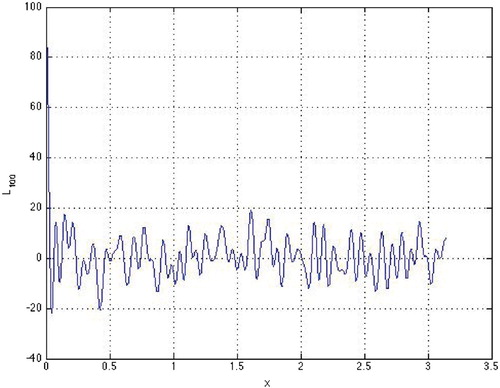
(2) ). Figure gives an example of a TP (Equation2
(2)
(2) ) of order 100 with the estimated number
of zeros located in
to be around 93.
Figure 1. TP ,
, with randomly distributed digits
.
Many approaches in the TP theory deal with introduction of various TP families and obtaining different sufficient conditions providing the existence of the TP zeros valid for each particular family or class of TPs. In many cases, the developed approaches enable one to describe distribution of zeros and determine their number (over a period). Let us give two examples illustrating such methods. In [Citation9] it is examined the size of a real TP of degree at most n having at least k zeros in R (mod
) (counting multiplicities). In [Citation14] the following sufficient conditions are obtained for the existence of zeros of a family of cosine TPs
(3)
(3) where
,
, is a monotonically decreasing (
,
) and convex (
,
) number sequence: TP (Equation3
(3)
(3) ) has one simple zero on every interval
,
.
An example of the TP generalization according to [Citation11] has the form
(4)
(4) where
is a continuous function with positive (or negative, but not both) first derivative for x real. In particular,
,
, are the Chebyshev polynomial of degree k.
Cylindrical polynomials (CPs) have much in common with TPs; however, their theory is much less developed. CPs occur when particular solutions to Maxwell equations are sought in polar or cylindrical coordinates in domains where boundary and interface contours or surfaces possess circular symmetry. Standard reference books on cylindrical functions (see e.g. [Citation15–17]) consider two-term sums of products of two cylindrical functions occurring, e.g. in the form [Citation18,Citation19] (
) of cross-products of Bessel functions. Extension to the greater number of factors in the products or greater number of product terms has not been performed, to the best of our knowledge.
This study follows and contribute to the three main directions of the TP and CP theories: creating a universal form of generalized TPs; extension of the methods of the TP analysis to the class of CPs involving cylindrical functions of different kinds and order; and obtaining new sufficient conditions providing the existence and description of distribution of zeros of certain families of TPs and CPs. The latter employs non-periodic TPs and analysis of their parameter dependence.
Another objective is application of the obtained results in the electromagnetic field theory, namely, to the determination of real and complex oscillations and waves. The latter are reduced to multi-parameter eigenvalue problems [Citation20,Citation21] and then in many cases (when, e.g. the Helmholtz equation admits closed-form solutions using separation of variables) to dispersion equations (DEs). Their complete study is a sophisticated task which requires deep analytical–numerical investigations. In this work, a major attention is paid to creating an introduction to a general method that enables obtaining (sufficient) conditions of the existence and description of localization of the DE roots providing thus justification for the methods of determination of oscillations and waves in multi-layered structures which can be easily implemented in calculations. The method is based on the studies of the so-called generalized TPs GTPs
and generalized CPs
GCPs
aimed in particular to finding zeros of GTPs and GCPs using different approaches.
The approach proposed in this study makes use of the method [Citation22,Citation23] employing GCPs applied in [Citation23] to the rigorous analysis and determination of real waves in a dielectric waveguide (DW) and a Goubau line (GL) of circular cross section. The technique involves recursive procedures of the determination of zeros of TPs, GTPs, and GCPs.
2. Trigonometric polynomials
TPs are weighted linear combinations
(5)
(5) of complex exponents or trigonometric functions
(q=1) or
(q=2), where
(for
),
and
are integers forming integer 'frequency' parameter vectors
, and
and
(
, q=1,2) are constants or bounded continuous functions considered on the whole line, half-line x>0, or an interval. A cosine TP (Equation2
(2)
(2) ) considered by Littlewood has all
and is therefore
-periodic. One also separates the cases
and
or
and all
const (
) giving classical (
-periodic) TPs, even (a cosine TP with all
) or odd (a sine TP with all
). A 'regular' TP (Equation1
(1)
(1) ) constitutes, as well as TPs (Equation2
(2)
(2) )–(Equation4
(4)
(4) ), examples of such polynomials; several more are presented in the appendix.
Together with TPs (Equation5(5)
(5) ) we will study more general cases of non-periodic TPs considering wieghted trigonometric sums (TSs)
(6)
(6) with generally non-integer ‘frequency’ parameter vectors
, q=1,2. TS (Equation6
(6)
(6) ) is a TP having the form (Equation5
(5)
(5) ) of the order
.
Many standard examples of TPs and TSs calculated in the closed form for which it is possible to determine all zeros explicitly are considered in the appendix.
3. Cylindrical polynomials
In this study, we call CPs the weighted linear combinations
(7)
(7) of cylindrical functions
, where each
is either Bessel,
, or Neumann,
, function (
),
are real numbers forming parameter vectors
, and
(
) are constants or bounded continuous functions considered on the whole line, half-line x>0, or an interval. Unlike classical
-periodic TPs and TSs (EquationA1
(A1)
(A1) )–(EquationA6
(A6)
(A6) ) with integer parameter vectors, CPs (Equation7
(7)
(7) ) are non-periodic (and in this respect they are similar to TPs (Equation6
(6)
(6) )) although every term in (Equation7
(7)
(7) ) is an almost-periodic function. Namely, the following statements hold: (i) every function
has a countable sequence of positive simple zeros
increasing w.r.t. index k; (ii) the distance
(
) between two neighboring zeros of
tends to a constant (in particular, to π for the Bessel functions) as
; (iii) there is a number r>0 such that
(
); and (iv) zeros of every two different cylindrical functions
,
,
,
(
), or
,
(
) alternate.
Analysis of CPs including the existence and distribution of their (real or complex) zeros constitutes a specific set of complicated mathematical problems that has been rarely addressed in the literature as compared with TPs (where one may refer, e.g. to [Citation1,Citation2,Citation10,Citation12]).
4. Generalized TPs and CPs
Consider weighted linear combinations
(8)
(8) or
(9)
(9) of the products
or
of trigonometric,
, or cylindrical,
, functions, where
,
and
are constants or bounded continuous functions for x>0 and
and
are real parameters forming the ‘frequency’ parameter vectors
and
,
.
In this study, functions (Equation8(8)
(8) ) or (Equation9
(9)
(9) ) are referred to, respectively, as generalized TPs (GTPs) or GCPs of order
. In particular, for TPs (Equation5
(5)
(5) ) and (Equation6
(6)
(6) )
(10)
(10) all
so that they are GTPs of order
with
.
In the studies of cylindrical functions (e.g. in [Citation15–17]) zeros are considered of the two-term sums of products of two cylindrical functions; that is, of , where
with
denoting the order of two cylindrical functions
and
that have either different kind, or the same kind and different order or different parameters
and
(m=1,2). Such two-term sums of products, e.g.
(
) as in [Citation19] are called cross-product Bessel functions.
Lemma 4.1
A product of trigonometric functions
can be represented as a GTP of order
with a certain
, that is, as a TP (Equation6
(6)
(6) ) of order
.
Proof.
The first step of the induction proof is to check basic trigonometric identities ,
, and
and to apply them to the triple products, e.g.
so that
with
,
,
,
,
,
, and
.
Assuming now that
(11)
(11) one can easily verify, after converting each product of two trigonometric functions to a sum, that
Corollary 4.2
A GTP (Equation8(8)
(8) ) of order
can be represented as a TP (Equation6
(6)
(6) ) of a certain order
.
Proof.
Every product in (Equation8
(8)
(8) ) can be written according to Lemma 4.1 as a GTP of order
with a certain
. Consequently, GTP (Equation8
(8)
(8) ) of order
can be represented as a sum of TPs (Equation6
(6)
(6) ) and finally as a TP (Equation6
(6)
(6) ) of the order
.
Lemma 4.3
Denote by and
,
, intervals formed by two pairs of neighboring positive zeros of
and
given by (EquationA9
(A9)
(A9) ) and (EquationA10
(A10)
(A10) ) with
. Then for any three distinct positive numbers
,
, and
,
, there are
,
, and integers
and
such that
and
or
and
.
Proof.
Endpoints of and
form equidistant (uniform) grids of points on the half-line
separated by
and
. Therefore, there is an interval between certain neighboring grid points of each grid that contains one, two, or three of the numbers
,
, and
(we assume that
does not coincide with any of the grid points). Choosing
or
such that
we see that there are integers
and
such that
or
and
.
5. Zeros of GTPs and GCPs
In order to formulate sufficient conditions that guarantee the existence of zeros of GTPs and GCPs and describe their localization, we will use the following
Lemma 5.1
Let , j=1,2,3 (continuous in a closed interval
),
, and
or, equivalently, there is an
such that
; then the equation
has a root
.
Proof.
Indeed, and
so that
and therefore
has a root
.
5.1. GTPs
We have already noted that TPs (EquationA1(A1)
(A1) )–(EquationA6
(A6)
(A6) ) have each infinitely many zeros for any number of their terms
and that infinitely many zeros of 'neighboring' TPs
,
,
,
, and
,
(
) alternate. This statement can be in a certain sense generalized for arbitrary GTP using Lemma 5.1, validating simultaneously a recursive procedure of proving the existence and determining the location of zeros of TPs, GTPs, and GCPs.
Theorem 5.2
There are (in general, non-integer) frequency vectors , q=1,2, such that a TP (Equation6
(6)
(6) ) of order
where
are arbitrary constants or bounded continuous functions that do not vanish on the half-line x>0 has a positive zero.
Proof.
The first step of the induction proof is to call that TPs of orders 1 and 2, ,
, and
, have each infinitely many positive zeros for any
const,
, and
, q=1,2. The latter statement is easily extended to the case when
are any two functions satisfying the condition of the theorem. Next, assume that TP
in the form (Equation6
(6)
(6) ) of order
has a positive zero
and consider TPs of order 2M−1
(12)
(12)
(13)
(13)
Applying Lemmas 4.3 and 5.1 with
being an interval formed by two neighboring zeros of
or
and choosing
or
in line with Lemma 4.3 with respect to
we prove the statement of the theorem.
Statement of Theorem 5.2 is valid for cosine TP (Equation2(2)
(2) ) considered by Littlewood in the form stronger than that for non-periodic TPs and GTPs. Namely, one can estimate the number of zeros on half-period
and establish the existence of infinitely many positive zeros of TP (Equation2
(2)
(2) ).
Corollary 5.3
TP (Equation2(2)
(2) ) of order
where
and
,
, are two aribtrary
different
integers, has at least
zeros on half-period
and infinitely many positive zeros.
Proof.
The first step of the induction proof is to call that TPs (Equation2(2)
(2) ) of orders 1 and 2,
and
, have each infinitely many positive zeros
(14)
(14) for any integers
,
, and
,
, with
; in particular,
has
zeros and
has
(when parity of
and
is the same) or
(parity of
and
is different) zeros on half-period
. Thus, zeros of
form a finite set of distinst points on the interval
. To show details of the proof of the induction step, consider
. According to Lemma 4.3, one can choose
such that intervals
,
(where
or
) between two neighboring zeros of
contain each one zero of
. This means, in line with Lemma 5.1, that
has a zero on each
. Consider now
and assume that
are L
zeros of
on
. According to Lemma 4.3, one can choose
such that intervals between two neighboring zeros of
contain each one zero of
. Therefore, Lemma 5.1 implies that the corollary is proved.
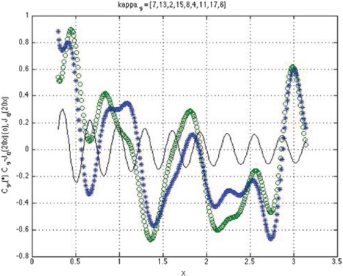
Figures and illustrate the proofs and display examples of TPs (Equation2(2)
(2) ) of different orders. Comparing Figures and one observes a clear similarity between CPs and TPs with respect to the statements of Theorems 5.2 and 5.4 and Lemma 4.3.
Figure 2. TPs (M=3,
,
,
) with
,
;
(o) has 7 zeros located together with 7 zeros of
(*) between pairs of neighboring zeros of
.
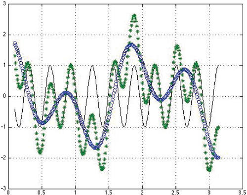
Figure 3. TPs (lower curve with greater number of oscillations) with
,
(upper curve with greater number of oscillations), and
,
; zeros of TPs alternate and
and
have each 11 zeros located between pairs of neighboring zeros of
.
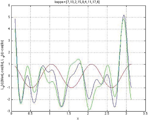
Figure 4. CPs with
,
;
(o) has 4 zeros located together with 6 zeros of
(*) between pairs of neighboring zeros of
.
5.2. GCPs
According to Corollary 4.2, Theorem 5.2 can be applied to GTP (Equation8(8)
(8) ). However it is reasonable to give an independent proof which provides sufficient conditions of the existence of zeros of both GTPs (Equation8
(8)
(8) ) and GCPs (Equation9
(9)
(9) ).
Theorem 5.4
There are ‘frequency’ vector sets and
, where
and
(
) have real components, such that GTP (Equation8
(8)
(8) ) and GCP (Equation9
(9)
(9) ) of order
where
and
(
) are arbitrary constants or bounded continuous functions that do not vanish on the half-line x>0 have each a positive zero.
Proof.
First, note that at M=1, GTP (Equation8(8)
(8) ) and GCP (Equation9
(9)
(9) ) of order
are single products having each (as a function of x) infinitely many positive zeros forming countable sets
and
being unions of the infinite sets
and
of the zeros
and
(
) of all
and
that enter these products.
Second, for any and
, the products
and
comprising
factors have each infinitely many positive zeros forming countable sets
and
being unions of the infinite sets
and
of the zeros
and
(
) of all
and
. Elements of
and
(and of
and
) depend on the parameter vectors
and
(
).
Perform the next step of induction and represent GTP (Equation8(8)
(8) ) and GCP (Equation9
(9)
(9) ) as
(15)
(15)
(16)
(16)
where
,
and
vanish at the endpoints of the intervals
and
(
) between every two their neighboring zeros.
Assume that the parameter vector sets and
in (Equation15
(15)
(15) ) and (Equation16
(16)
(16) ) are such that GTP
and GCP
of order
have each a zero
or
. Choose
and
according to Lemma 4.3 with
being intervals
or
formed by two neighboring zeros of
or
with index pairs
or
such that
or
. Next, use Lemma 5.1 to conclude that GTP (Equation8
(8)
(8) ) and GCP (Equation9
(9)
(9) ) of order
have each a zero on these intervals proving thus the statement of the theorem.
6. Application to DEs in electromagnetic field theory
6.1. Waveguides with circularly symmetric layered media
When electromagnetic wave propagation is considered [Citation20,Citation24] in waveguides having circular symmetry, like DWs or GLs formed by several concentric layers of media, all the field components of symmetric and non-symmetric waves are expressed [Citation21,Citation24] via a potential function which is sought generally as a linear combination of cylindrical functions of order
. This fact enables one to reduce finally the determination of the wave propagation constants to the solution of DEs involving CPs and GCPs. Further stages of the mathematical model are described in the next section.
6.1.1. Sturm–Liouville problems
Analysis of running (normal) waves in waveguides filled with circularly symmetric layered media is reduced [Citation21,Citation22,Citation25] to the non-selfadjoint Sturm–Liouville problems for the Bessel equation with piecewise constant coefficients on the semi-axis
(17)
(17)
(18)
(18)
(19)
(19)
here
β is the wave propagation constant (spectral parameter of the problem), ε and
are, respectively (real or complex) permittivity of the media and wavenumber of vacuum (a real parameter), and
with
are given expicitly for a particular structure.
Finding eiganvalues of (Equation17(17)
(17) ) and (Equation18
(18)
(18) ) (propagation constants of running waves) is reduced [Citation20–26] to the solution of functional equations w.r.t. spectral parameter γ or
usually called DEs. When real spectrum of problems (Equation17
(17)
(17) ) and (Equation18
(18)
(18) ) is considered, the quantities are sought as real-valued functions of real spectral parameter γ (or λ) varying on a certain interval
.
For multi-layered DWs or GLs when the number M>1 of dielectric layers (that is, discontinuities of the coefficient in the differential equations entering (Equation17(17)
(17) ) and (Equation18
(18)
(18) )) may be arbitrary, transmission conditions in (Equation17
(17)
(17) ) and (Equation18
(18)
(18) ) comprise
jump relations with different
at the layer boundaries
,
, for DW or
,
(
), for GL.
The general results of the classical Sturm–Liouville theory concerning the existence and distribution of (real or complex) spectrum for this type of problems are not applicable because the boundary (transmission) conditions depend on the spectral parameter; this dependence which is specified by concrete functions obtained explicitly governs the presence or absence of spectrum.
The explicit expressions for the DEs obtained in [Citation22–24] for multi-layered DWs and GLs (open or shielded) or structures formed by plane-parallel layers of media [Citation27,Citation28] show that these DEs involve GCPs where weight coefficients and
are constants or bounded continuous functions for x>0 determined explicitly and
and
forming the parameter vectors
and
,
are real quantities expressed in terms of parameters of the particular structure (Figure ).
Figure 5. Zeros of a GCP (curve with highest oscillation) given by (Equation21
(21)
(21) ) situated between neighboring zeros of
(curve with a negative starting value) and
(curve with a positive starting value).

6.1.2. Single-layer DW and GL
The DEs for single-layer DW and GL can be represented [Citation21–23,Citation25,Citation26] in the general form involving GCPs (Equation9(9)
(9) )
(20)
(20)
(21)
(21)
where
,
and
(m=0,1) are the Bessel, Neumann, and Macdonald functions,
,
and
are Bessel cross-products [Citation19], and the waveguide geometric and material parameters
,
,
,
(β, ε, and
are, respectively, the wave progation constant, permittivity, and free-space wavenumber),
, and
(a and b are characteristic dimensions of DW and GL).
For a GCP in (Equation21
(21)
(21) ) we can apply this reasoning and Lemma 5.1 by setting
and
. Then
has a zero between every two neighboring zeros
and
of
as soon as q>1 is such that a zero of
belongs to the interval
. The latter condition can be satisfied because zeros
of
alternate for different j=1,2 and form sequences of points decreasing with respect to q [Citation21,Citation22,Citation26]. The conclusion concerning the existence and location of the zeros of
between neighboring alternating zeros of
and
is perfectly illustrated by Figure .
Straightforward analysis of (Equation20(20)
(20) ) and (Equation21
(21)
(21) ) demonstrates that functions
and
entering DEs have distinct common features: they are sums of (products of) cylindrical functions
and
each having infinitely many alternating simple positive zeros. The latter yields an immediate proof (illustrated by Figure and verified below) of the (sufficient conditions) providing the existence of real roots of the DEs located between zeros of
and
(m=0,1). The existence, localization, and number of the DE roots are governed actually by a number of zeros of
or
that are inside the domain
of
and
; that is, by the value of parameter u.
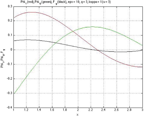
Figure 6. Example for a GCP in DE (Equation20
(20)
(20) ): plots of
(upper curve with no oscillations),
(lower curve with no oscillations), and
(curve with one oscillations) at
and
(
) displaying a zero of
between neighboring zeros of
and neighboring zeros of
and
.
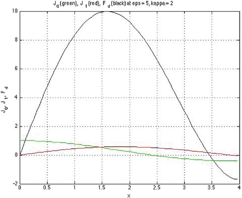
Figure 7. An example showing alternating zeros of (curve starts at −0.3),
(curve starts above 0.2), and
(curve starts above 0).
6.1.3. Multi-layered waveguides
For M-layer DWs or GLs with M>1 DE takes the form [Citation29] of the determinant equation
(22)
(22) where
is a one-to-one function of the spectral parameter considered on a certain interval
and
are cylindrical functions, either of different order or type or with different parameter factors
(
).
Thus, solution to Equation (Equation22(22)
(22) ) reduces to the determination of zeros of a GCP (Equation9
(9)
(9) ) obtained as a result of calculation of the determinant. The GCP involves products
of the cylindrical functions entering (Equation22
(22)
(22) ).
A is a block-diagonal matrix obtained explicitly in [Citation29] which yields the possibility of recursive computation of its determinant and obtaining formulas similar to (Equation15(15)
(15) )
(23)
(23) using low-order minors
and cofactors so that at the first (and each subsequent) recursive step the expression for
contains two terms. This enables one to apply the procedure outlined in the proof of Theorem 5.4: Assume that parameter
in (Equation23
(23)
(23) ) is such that an interval
formed by two neighboring zeros of
with index
contains one particular zero of
. Such a choice of parameter is possible because each
, p=1,2, has infinitely many zeros forming almost periodical sequences and each zero (as well as the distance between any two neighboring zeros) is a monotonically decreasing function of
.
Next, we use Lemma 5.1 to conclude that in (Equation23
(23)
(23) ) has a zero on the interval
6.2. Plane-parallel layered guiding structures
Determining resonant states and eigenfrequencies of plane-parallel layered dielectrics in free space, between parallel perfectly conducting planes, or in a waveguide of rectangular cross section is considered in terms of non-selfadjoint Sturm–Liouville problems (Equation17(17)
(17) ) for the equation
on the line with piecewise constant coefficients; eigenfunctions
are sought as a linear combination of trigonometric functions
and the problem in question is reduced [Citation27,Citation28] to DEs involving complex-valued TPs
(24)
(24) here z is a real or complex variable associated with one particular layer in an M-layer structure (e.g.
with s being the index of the layer with permittivity
,
) and
are complex-valued functions depending on all the problem parameters. In particular, for the single-layer structure (comprising one dielectric slab), we have [Citation27]
(25)
(25) where t>0 and C>0 are (real) parameters. In [Citation27], it is proved that
is an entire even function, the DE
has no real zeros and has infinitely many complex zeros located in pairs in the first and third quadrants in the complex z-plane. This result is extended to M-layer plane-parallel structures. Explicit (tedious) expressions for
in the cases of two and three layers may be found in [Citation27].
7. Conclusion
We have developed the theory of TPs and proposed a generalization of the notion of TP that can be applied to the analysis of CPs.
The proposed method is based on the introduction and analysis of GTPs and GCPs. The technique can be applied in electromagnetics using the explicit forms of DEs expressed as weighted sums of products of trigonometric and cylindrical functions that describe eigenoscillations and normal waves in layered structures. The approach enables one to complete rigorous proofs of existence and determine domains of localization of the DE roots and validate iterative numerical solution techniques.
The obtained results complete mathematical theory of DEs for multi-layered waveguides possessing circular or plane-parallel symmetry and can be extended to more general structures as well as to determination of complex waves.
Disclosure statement
No potential conflict of interest was reported by the author.
References
- Milovanovic GV, Mitrinovic DS, Rassias ThM. Topics in polynomials: extremal problems, inequalities, zeros. Singapore: World Scientific; 1994.
- Littlewood JE. Some problems in real and complex analysis, heath mathematical monographs. Lexington (MA); 1968.
- Davis PJ. Interpolation and approximation. New York: Blaisdell; 1968.
- Dumitrescu DA. Positive trigonometric polynomials and signal processing applications. Springer; 2007.
- Chanane B. Computing the spectrum of non-selfadjoint Sturm Liouville problems with parameter-dependent boundary conditions. J Comp Appl Maths. 2007;206(1):229–237. doi: 10.1016/j.cam.2006.06.014
- Littlewood JE. On the real roots of real trigonometrical polynomials (II). J Lond Math Soc. 1964;39:511–552. doi: 10.1112/jlms/s1-39.1.511
- Littlewood JE. The real zeros and value distributions of real trigonometrical polynomials. J Lond Math Soc. 1966;41:336–342. doi: 10.1112/jlms/s1-41.1.336
- Erdelyi T. Polynomials with littlewood-type coefficient constraints. In: Chui CK, Schumaker LL, Stoeckler J, editors. Approximation theory X. Nashville, TN: Vanderbilt University Press; 2001. p. 1–40.
- Borwein P, Erdelyi T. Trigonometric polynomials with many real zeros and a littlewood-type problem. Proc Am Math Soc. 2000;129(3):725–730. doi: 10.1090/S0002-9939-00-06021-4
- Lanczos C. Trigonometric interpolation of empirical and analytical functions. J Math Phys. 1938;17:123–199. doi: 10.1002/sapm1938171123
- Oliveira-Pinto F. Experiments with a class of generalized trigonometric polynomials. Calcolo. 1984;21(3):253–268. doi: 10.1007/BF02576536
- Polya G, Szegö G. Aufgaben und Lehrsätze aus der Analysis. 3rd ed. Berlin: Springer; 1964.
- Borwein P, Erdelyi T, Ferguson R, et al. On the zeros of cosine polynomials: solution to a problem of littlewood. Ann Math. 2008;167:1109–1117. doi: 10.4007/annals.2008.167.1109
- Runovsky VK. On real zeros of an even trigonometric polynomial. Mat Zametki. 1988;43(3):334–336.
- Watson GN. Theory of bessel functions. 2nd ed. New York: Cambridge University Press and Macmillan Co.; 1948.
- Jahnke E, Emde F. Tables of functions. 4th ed. New York: Dover Publications; 1945.
- Abramowitz M, Stegun IA., editors. Handbook of mathematical functions with formulas, graphs, and mathematical tables. New York: Dover; 1972.
- NIST Digital Library of Mathematical Functions. Release 1.0.20 of 2018-09-15. F. W. J. Olver, A. B. Olde Daalhuis, D. W. Lozier, B. I. Schneider, R. F. Boisvert, C. W. Clark, B. R. Miller, and B. V. Saunders, eds.
- Ek JM, Thielman HP, Huebschman EC. On the zeros of cross-product bessel functions. J Math Mech. 1966;16(5):447–452.
- Snyder AW, Love J. Optical waveguide theory. Springer; 1983.
- Shestopalov Y, Kuzmina E, Samokhin A. On a mathematical theory of open metal-dielectric waveguides. FERMAT. 2014;5.
- Shestopalov Y, Kuzmina E. Symmetric surface complex waves in Goubau line. Cogent Eng. 2018;5(1):1–16.
- Shestopalov Y, Kuzmina E. Complex waves in multi-layered metal-dielectric waveguides. Proc. 2018 Int. Conf. Electromagnetics in Advanced Application (ICEAA), 20th Edition, Cartagena de Indias, Colombia: September 10–14, 2018. p. 122–125.
- Weinstein LA. Open resonators and open waveguides. Golem Press; 1969.
- Shestopalov Y. Complex waves in a dielectric waveguide. Wave Motion. 2018;57:16–19. doi: 10.1016/j.wavemoti.2018.07.005
- Ismail MEH, Muldoon M. Monotonicity of the zeros of a cross-product of bessel functions. SIAM J Math Anal. 1978;9(4):759–767. doi: 10.1137/0509055
- Shestopalov Y. Resonant states in waveguide transmission problems. PIER B. 2015;64(1):119–143. doi: 10.2528/PIERB15083001
- Shestopalov Y. Singularities of the transmission coefficient and anomalous scattering by a dielectric slab. J Math Phys. 2018;59(3):033507. doi: 10.1063/1.5027195
- Karchevskii EM, Beilina L, Spiridonov AO, et al. Reconstruction of dielectric constants of multi-layered optical fibers using propagation constants measurements, arXiv: 1512.06764v1 [math.NA], Dec. 2015.
Appendix
The Fejer kernel
(A1)
(A1) the Dirichlet kernel
(A2)
(A2) and other trigonometric sums like
(A3)
(A3) a cosine TP with all
,
, and the parameter vector
(A4)
(A4) a sine TP with all
,
, and the parameter vector
(A5)
(A5) a TP with all
(A6)
(A6) ‘shifted’ TPs (EquationA4
(A4)
(A4) ), (EquationA5
(A5)
(A5) ) with all
and
(A7)
(A7)
and all
and
(A8)
(A8)
are examples of TPs which can be calculated in the closed form involving only products of trigonometric functions. This enables one to obtain all zeros of TPs (EquationA1
(A1)
(A1) )–(EquationA6
(A6)
(A6) )
(limiting ourselves only to positive zeros,
).
Zeros
(A9)
(A9)
(A10)
(A10)
of all intermediate terms
and
in TPs (EquationA1
(A1)
(A1) )–(EquationA6
(A6)
(A6) ) alternate with
,
,
,
, and
. In fact, excluding, e.g. merging zeros of (EquationA6
(A6)
(A6) )
when
(A11)
(A11) which is valid particularly for
,
, we have that zeros of (EquationA6
(A6)
(A6) ) are all different if condition (EquationA11
(A11)
(A11) ) does not hold. Another valuable observation is that infinitely many zeros of
,
,
,
, and
,
(
) alternate.
Also, the distances and
between neigboring zeros of
,
, and
are less than the distance
between neigboring zeros of
and
(
) for
.