The Ekman spiral for piecewise-constant eddy viscosity

ABSTRACT

We investigate the classical problem of wind-stress-induced non-equatorial steady ocean currents, considering a three-valued piecewise-constant eddy viscosity. This extends and generalizes recent results on piecewise-uniform eddy viscosity with only two layers. The aim is to determine how variations in the relative values of the eddy viscosity at different depths may account for the deviations from the surface current deflection of 45${}^{\circ }$, predicted in the classical constant eddy viscosity case. Such variations are observed in field data, and we investigate analytically the effect the presence of a third region makes compared to the two-layer case.

Keywords:

• Boundary-value problem
• viscous flow
• wind-driven currents
• deflection angle

AMS CLASSIFICATIONs:

• 34B05
• 34B40
• 35Q35
• 76U05

1. Introduction

The circulation in the ocean is due to two main processes. Firstly, the tangential stress of surface wind generates currents that are generally confined to relatively small depths (wind-driven circulation); secondly, convective motions caused by temperature gradients or salt inputs are responsible for the (much slower) ventilation of the abyss (thermohaline circulation) (cf. [1]). In this paper we shall focus on the former aspect of ocean circulation.

It is crucial to distinguish between equatorial and non-equatorial flows, because their respective behaviours differ substantially from each other and thus essentially different methods and models are employed in their analysis. This is due to the fact that the change of sign of the Coriolis force across the Equator yields an effective waveguide, which enhances azimuthal (i.e. longitudinal) flow propagation along the Equator (see [2–4]). Moreover, at non-equatorial latitudes, where the Coriolis force is larger, the flow beneath a relatively thin surface boundary layer is mainly in geostrophic balance (that is, the force balance occurs between the Coriolis force and horizontal pressure gradients), whereas at equatorial latitudes, where the Coriolis force vanishes, geostrophic effects are negligible and nonlinear effects arise at leading order, so that for equatorial wind-drift currents a completely different approach is required. In the following we restrict ourselves to the non-equatorial setting. For recent result on equatorial flows we refer to [5–7], in addition to the references above.

As already mentioned, at non-equatorial latitudes the oceanic flow below a depth of about 100 metres or so is, to a good degree of approximation, in geostrophic balance. However, closer to the surface, wind-generated turbulence in the water carries the momentum of the wind down to the interior, thus inducing currents (superimposed to the underlying geostrophic flow) where the force balance is between the Coriolis force and the frictional forces due to the wind. The layer where these frictional effects are significant is called the Ekman layer and is named after the Swedish scientist who first formulated and analysed a mathematical model describing the behaviour of wind-generated steady surface currents. In his pioneering work [8], published in 1905, Ekman modelled the frictional effects by introducing an (in general depth-dependent) eddy viscosity coefficient (see the next section); in the simplest setting of constant eddy viscosity, he came to the following conclusions:

1. The induced surface current is deflected to the right of the direction of the generating wind by an angle of 45${}^{\circ }$ in the Northern Hemisphere (to the left in the Southern Hemisphere).

2. With increasing depth, the velocity of the current decays in magnitude and is further deflected in clockwise (anticlockwise) direction in the Northern (Southern) Hemisphere, following a spiral (now called an Ekman spiral).

3. The net mass transport of the current is directed at right angle to the right (left) of the direction of the wind in the Northern (Southern) Hemisphere.

Properties (ii) and (iii) have been shown to hold in the general case of depth-dependent eddy viscosity (see [9]); however, property (i) is not valid in general and agrees only qualitatively (i.e. it predicts the correct direction of deflection) but not quantitatively with direct observations, which measure deflection angles in the range 10${}^{\circ }$–75${}^{\circ }$ (cf. the data in [10] or [11]). It is reasonable to identify the simplified assumption of constant vertical eddy viscosity as the source for the inaccuracy in the prediction of the value of the deflection angle, but investigating how exactly a change in the eddy viscosity affects the deflection angle is very complicated and explicit solutions to other more general cases are scarce; most of the known ones can be found in [12–14]. The perturbative approach pursued in [9,15] in order to determine whether a given small perturbation of a constant eddy viscosity leads to a positive or negative increment of the deflection angle gives a good idea of how intricate the investigation of this problem is. Nevertheless, an analysis of situations that do not require the smallness assumptions required for a perturbative approach is of great interest. Wind-induced oceanic surface currents play a decisive role in the heat transport between different geographic regions and have a direct impact on the global climate (see [1]). Therefore, gaining a better understanding of their behaviour would be also of fundamental practical interest.

In [16], the authors construct an explicit solution in the case of a piecewise-constant eddy viscosity with two distinct values, and investigate how variations in the ratio of the two values affect the deflection angle at the surface. In this paper, we focus on the more general case of a three-valued piecewise constant eddy viscosity. The two-valued case is suited for the situation where a thin upper layer is situated on top of an abyssal one; in the three-valued case we are considering, there are two relatively thin regions over a third, much deeper one. Our goal is thus to see in detail how the presence of the extra middle layer affects the general behaviour of the surface deflection angle. We are interested in a thorough and precise mathematical description, and the methods we use are rigorously analytical; at some points, the discussion is supported by basic numerical plots that help visualizing the involved behaviour of the analytical solution we derive.

The paper is organized as follows. First, we present a concise derivation of the equation we aim to solve (after we non-dimensionalize it properly). In the subsequent section, we construct an explicit solution for the case of three regions of piecewise-constant eddy viscosity and use it to write down a formula for the surface deflection angle. Finally, we discuss the properties of the formula we have found for the deflection angle, with particular attention for the differences between the two-valued and the three-valued case.

2. The governing equations

The horizontal equations of motion for steady flow under the f-plane approximation (see [17]), written out in components, are (1) $\begin{array}{rl}-fV& =\frac{1}{\rho }\frac{\mathrm{\partial }{\tau }_x}{\mathrm{\partial }Z}-\frac{1}{\rho }\frac{\mathrm{\partial }P}{\mathrm{\partial }X}+\text{higher order terms}\end{array}$(1) (2) $\begin{array}{rl}fU& =\frac{1}{\rho }\frac{\mathrm{\partial }{\tau }_y}{\mathrm{\partial }Z}-\frac{1}{\rho }\frac{\mathrm{\partial }P}{\mathrm{\partial }Y}+\text{higher order terms},\end{array}$(2) where ρ is the (constant) density of the water, $(U,V)$ is the horizontal velocity in the $(X,Y)$ plane, Z is the depth below the mean level Z = 0 (the Z-axis pointing upward, so that Z will be negative), f is the Coriolis parameter, P is the pressure, and $({\tau }_x,{\tau }_y)$ is the shear stress vector. The higher order terms represent interactions between the variables and are supposed to be negligible. We may introduce the complex notation $\mathbf{U}=U+\mathrm{i}V$, $\tau ={\tau }_x+\mathrm{i}{\tau }_y$, and $\mathrm{\nabla }P=\mathrm{\partial }P/\mathrm{\partial }X+\mathrm{i}\mathrm{\partial }P/\mathrm{\partial }Y$, which enables us to rewrite (1(1) $\begin{array}{rl}-fV& =\frac{1}{\rho }\frac{\mathrm{\partial }{\tau }_x}{\mathrm{\partial }Z}-\frac{1}{\rho }\frac{\mathrm{\partial }P}{\mathrm{\partial }X}+\text{higher order terms}\end{array}$(1) ) and (2(2) $\begin{array}{rl}fU& =\frac{1}{\rho }\frac{\mathrm{\partial }{\tau }_y}{\mathrm{\partial }Z}-\frac{1}{\rho }\frac{\mathrm{\partial }P}{\mathrm{\partial }Y}+\text{higher order terms},\end{array}$(2) ) (ignoring the higher order terms) as (3) $\mathrm{i}f\mathbf{U}=\frac{1}{\rho }\frac{\mathrm{\partial }\tau }{\mathrm{\partial }Z}-\frac{1}{\rho }\mathrm{\nabla }P.$(3) Splitting $\mathbf{U}$ into a geostrophic (${\mathbf{U}}_{\mathrm{g}}$) and a wind-driven (Ekman) component (${\mathbf{U}}_{\mathrm{e}}$), i.e. $\mathbf{U}={\mathbf{U}}_{\mathrm{g}}+{\mathbf{U}}_{\mathrm{e}}$, we obtain from (3(3) $\mathrm{i}f\mathbf{U}=\frac{1}{\rho }\frac{\mathrm{\partial }\tau }{\mathrm{\partial }Z}-\frac{1}{\rho }\mathrm{\nabla }P.$(3) ) the following equation for ${\mathbf{U}}_{\mathrm{e}}$: (4) $\mathrm{i}f{\mathbf{U}}_{\mathrm{e}}=\frac{1}{\rho }\frac{\mathrm{\partial }\tau }{\mathrm{\partial }Z}.$(4) The right-hand side of this equation can be related to ${\mathbf{U}}_{\mathrm{e}}$ through $\tau =\rho \nu \frac{\mathrm{\partial }{\mathbf{U}}_{\mathrm{e}}}{\mathrm{\partial }Z},$where $\nu =\nu \left(Z\right)$ is the depth-dependent vertical eddy viscosity coefficient (cf. [18,19]); plugging this into (4(4) $\mathrm{i}f{\mathbf{U}}_{\mathrm{e}}=\frac{1}{\rho }\frac{\mathrm{\partial }\tau }{\mathrm{\partial }Z}.$(4) ) yields (5) $\mathrm{i}f{\mathbf{U}}_{\mathrm{e}}=\frac{\mathrm{\partial }}{\mathrm{\partial }Z}\left(\nu \frac{\mathrm{\partial }{\mathbf{U}}_{\mathrm{e}}}{\mathrm{\partial }Z}\right).$(5) Appropriate boundary conditions are the following. On the surface, (6) ${\tau }_0=\rho \nu \frac{\mathrm{\partial }{\mathbf{U}}_{\mathrm{e}}}{\mathrm{\partial }Z}\text{on }Z=0,$(6) i.e. there the shear stress is balanced by the (constant) wind stress ${\tau }_0$. Moreover, the condition (7) ${\mathbf{U}}_{\mathrm{e}}\to 0\text{as }Z\to -\mathrm{\infty }$(7) describes the fact that at large depths the wind-induced current is negligible compared to the underlying geostrophic flow.

Let ${\tau }_0$ denote the absolute value of the complex number ${\tau }_0$. Equation (5(5) $\mathrm{i}f{\mathbf{U}}_{\mathrm{e}}=\frac{\mathrm{\partial }}{\mathrm{\partial }Z}\left(\nu \frac{\mathrm{\partial }{\mathbf{U}}_{\mathrm{e}}}{\mathrm{\partial }Z}\right).$(5) ), together with the boundary conditions (6(6) ${\tau }_0=\rho \nu \frac{\mathrm{\partial }{\mathbf{U}}_{\mathrm{e}}}{\mathrm{\partial }Z}\text{on }Z=0,$(6) ) and (7(7) ${\mathbf{U}}_{\mathrm{e}}\to 0\text{as }Z\to -\mathrm{\infty }$(7) ), can be non-dimensionalized by introducing the dimensionless eddy viscosity $K=f\rho \nu /{\tau }_0$, the velocity $\mathbf{u}={\mathbf{U}}_{\mathrm{e}}/\sqrt{2{\tau }_0/\rho }$, and the depth $z=Zf/\sqrt{2{\tau }_0/\rho }$. We then set $\psi =K\left(0\right)\mathbf{u}$. Without loss of generality, we may assume that ${\tau }_0={\tau }_0+\mathrm{i}0$ (this will not change the deflection angle, which is the argument of $\psi \left(0\right)$). Using these considerations the dimensional problem transforms to (8) $\begin{array}{rl}(K{\psi }^{\prime }{)}^{\prime }-2\mathrm{i}\psi =0& \mathrm{f}\mathrm{o}\mathrm{r}z<0,\end{array}$(8) (9) $\begin{array}{rl}{\psi }^{\prime }\left(0\right)=1& \mathrm{o}\mathrm{n}z=0,\end{array}$(9) (10) $\begin{array}{rl}\psi \to 0& \mathrm{a}\mathrm{s}z\to -\mathrm{\infty },\end{array}$(10) where the prime denotes a derivative with respect to z.

From now on, K will be piecewise-constant, assuming different values in the three layers $[-h_1,0]$, $[-h_2,-h_1)$ and $(-\mathrm{\infty },-h_2)$ for some constants $h_2>h_1>0$. If necessary, one can scale z further to bring K to the form (11) $K\left(z\right)=\left\{\begin{array}{ll}1& \text{for }z\in [-h_1,0],\\ {\ell }_1^2& \text{for }z\in [-h_2,-h_1),\\ {\ell }_2^2& \text{for }z\in (-\mathrm{\infty },-h_2)\end{array}\right.$(11) for ${\ell }_1,{\ell }_2\ge 0$ (the squares ${\ell }_1^2$ and ${\ell }_2^2$ are for convenience later on).

3. Constructing an exact solution

Taking (11(11) $K\left(z\right)=\left\{\begin{array}{ll}1& \text{for }z\in [-h_1,0],\\ {\ell }_1^2& \text{for }z\in [-h_2,-h_1),\\ {\ell }_2^2& \text{for }z\in (-\mathrm{\infty },-h_2)\end{array}\right.$(11) ) into account, Equation (8(8) $\begin{array}{rl}(K{\psi }^{\prime }{)}^{\prime }-2\mathrm{i}\psi =0& \mathrm{f}\mathrm{o}\mathrm{r}z<0,\end{array}$(8) ) becomes (12) $\begin{array}{rl}{\psi }^{″}-2\mathrm{i}\psi & =0\text{for }-h_1<z<0,\end{array}$(12) (13) $\begin{array}{rl}{\ell }_1^2{\psi }^{″}-2\mathrm{i}\psi & =0\text{for }-h_2<z<-h_1,\end{array}$(13) (14) $\begin{array}{rl}{\ell }_2^2{\psi }^{″}-2\mathrm{i}\psi & =0\text{for }-\mathrm{\infty }<z<-h_2,\end{array}$(14) with general solution $\psi \left(z\right)=\left\{\begin{array}{ll}A{\mathrm{e}}^{(1+\mathrm{i})z}+B{\mathrm{e}}^{-(1+\mathrm{i})z}& \text{for }-h_1<z<0,\\ C{\mathrm{e}}^{(1+\mathrm{i})z/{\ell }_1}+D{\mathrm{e}}^{-(1+\mathrm{i})z/{\ell }_1}& \text{for }-h_2<z<-h_1,\\ E{\mathrm{e}}^{(1+\mathrm{i})z/{\ell }_2}& \text{for }-\mathrm{\infty }<z<-h_2,\end{array}\right.$for some constants A, B, C, D, E to be determined with the help of the surface boundary condition (9(9) $\begin{array}{rl}{\psi }^{\prime }\left(0\right)=1& \mathrm{o}\mathrm{n}z=0,\end{array}$(9) ) and some continuity considerations; note that the bottom boundary condition (10(10) $\begin{array}{rl}\psi \to 0& \mathrm{a}\mathrm{s}z\to -\mathrm{\infty },\end{array}$(10) ) has already been used to exclude the exponentially growing part of the solution in the interval $(-\mathrm{\infty },-h_2)$. Condition (9(9) $\begin{array}{rl}{\psi }^{\prime }\left(0\right)=1& \mathrm{o}\mathrm{n}z=0,\end{array}$(9) ) implies (15) $(1+\mathrm{i})(A-B)=1.$(15) Requiring continuity of the solution at $z=-h_1$ and $z=-h_2$, i.e. $\psi (-h_1^{+})=\psi (-h_1^{-})\text{and}\psi (-h_2^{+})=\psi (-h_2^{-}),$yields (16) $\begin{array}{rl}A{\mathrm{e}}^{-(1+\mathrm{i})h_1}+B{\mathrm{e}}^{(1+\mathrm{i})h_1}& =C{\mathrm{e}}^{-(1+\mathrm{i})h_1/{\ell }_1}+D{\mathrm{e}}^{(1+\mathrm{i})h_1/{\ell }_1},\end{array}$(16) (17) $\begin{array}{rl}C{\mathrm{e}}^{-(1+\mathrm{i})h_2/{\ell }_1}+D{\mathrm{e}}^{(1+\mathrm{i})h_2/{\ell }_1}& =E{\mathrm{e}}^{-(1+\mathrm{i})h_2/{\ell }_2}.\end{array}$(17) Now let $ϵ>0$. If we integrate (8(8) $\begin{array}{rl}(K{\psi }^{\prime }{)}^{\prime }-2\mathrm{i}\psi =0& \mathrm{f}\mathrm{o}\mathrm{r}z<0,\end{array}$(8) ) on the interval $(-h_1-ϵ,-h_1+ϵ)$ and let $ϵ\to 0$, we obtain ${\psi }^{\prime }(-h_1^{+})={\ell }_1^2{\psi }^{\prime }(-h_1^{-});$analogously, ${\ell }_1^2{\psi }^{\prime }(-h_2^{+})={\ell }_2^2{\psi }^{\prime }(-h_2^{-}).$From these conditions on the derivatives of ψ at $z=-h_1$ and $z=-h_2$ it follows (18) $\begin{array}{rl}A{\mathrm{e}}^{-(1+\mathrm{i})h_1}-B{\mathrm{e}}^{(1+\mathrm{i})h_1}& =C{\ell }_1{\mathrm{e}}^{-(1+\mathrm{i})h_1/{\ell }_1}-D{\ell }_1{\mathrm{e}}^{(1+\mathrm{i})h_1/{\ell }_1},\end{array}$(18) (19) $\begin{array}{rl}C{\ell }_1{\mathrm{e}}^{-(1+\mathrm{i})h_2/{\ell }_1}-D{\ell }_1{\mathrm{e}}^{(1+\mathrm{i})h_2/{\ell }_1}& =E{\ell }_2{\mathrm{e}}^{-(1+\mathrm{i})h_2/{\ell }_2}.\end{array}$(19) Equations (15(15) $(1+\mathrm{i})(A-B)=1.$(15) )–(19(19) $\begin{array}{rl}C{\ell }_1{\mathrm{e}}^{-(1+\mathrm{i})h_2/{\ell }_1}-D{\ell }_1{\mathrm{e}}^{(1+\mathrm{i})h_2/{\ell }_1}& =E{\ell }_2{\mathrm{e}}^{-(1+\mathrm{i})h_2/{\ell }_2}.\end{array}$(19) ) constitute a linear system of five equations for the five unknowns $(A,B,C,D,E)$ that can be solved by standard means, obtaining $\begin{array}{rl}A& =\frac{1}{4}E{\mathrm{e}}^{-(1+\mathrm{i})h_2/{\ell }_2}{\mathrm{e}}^{(1+\mathrm{i})h_2}[\left(1+\frac{{\ell }_2}{{\ell }_1}\right)(1+{\ell }_1){\mathrm{e}}^{(1+\mathrm{i})(h_2-h_1)/{\ell }_1}\\ & +\left(1-\frac{{\ell }_2}{{\ell }_1}\right)(1-{\ell }_1){\mathrm{e}}^{-(1+\mathrm{i})(h_2-h_1)/{\ell }_1}],\\ B& =\frac{1}{4}E{\mathrm{e}}^{-(1+\mathrm{i})h_2/{\ell }_2}{\mathrm{e}}^{-(1+\mathrm{i})h_2}[\left(1+\frac{{\ell }_2}{{\ell }_1}\right)(1-{\ell }_1){\mathrm{e}}^{(1+\mathrm{i})(h_2-h_1)/{\ell }_1}\\ & +\left(1-\frac{{\ell }_2}{{\ell }_1}\right)(1+{\ell }_1){\mathrm{e}}^{-(1+\mathrm{i})(h_2-h_1)/{\ell }_1}],\\ C& =\frac{1}{2}E\left(1+\frac{{\ell }_2}{{\ell }_1}\right){\mathrm{e}}^{-(1+\mathrm{i})h_2/{\ell }_2}{\mathrm{e}}^{(1+\mathrm{i})h_2/{\ell }_1},\\ D& =\frac{1}{2}E\left(1-\frac{{\ell }_2}{{\ell }_1}\right){\mathrm{e}}^{-(1+\mathrm{i})h_2/{\ell }_2}{\mathrm{e}}^{-(1+\mathrm{i})h_2/{\ell }_1},\\ E& =2(1-\mathrm{i}){\mathrm{e}}^{(1+\mathrm{i})h_2/{\ell }_2}[\left(1+\frac{{\ell }_2}{{\ell }_1}\right){\mathrm{e}}^{(1+\mathrm{i})(h_2-h_1)/{\ell }_1}\left((1+{\ell }_1){\mathrm{e}}^{(1+\mathrm{i})h_1}-(1-{\ell }_1){\mathrm{e}}^{-(1+\mathrm{i})h_1}\right)\\ & +\left(1-\frac{{\ell }_2}{{\ell }_1}\right){\mathrm{e}}^{(1+\mathrm{i})(h_2-h_1)/{\ell }_1}\left((1-{\ell }_1){\mathrm{e}}^{(1+\mathrm{i})h_1}-(1+{\ell }_1){\mathrm{e}}^{-(1+\mathrm{i})h_1}\right){]}^{-1}.\end{array}$We are mainly interested in determining the surface deflection angle ${\theta }_0$, which is given by the relation (20) $\tan {\theta }_0=-\frac{\mathrm{\Im }\left(\psi \right(0\left)\right)}{\mathrm{\Re }\left(\psi \right(0\left)\right)}=-\frac{\mathrm{\Im }(A+B)}{\mathrm{\Re }(A+B)}.$(20) Introducing the notation $\begin{array}{rl}\alpha & =(1+{\ell }_1){\mathrm{e}}^{h_1},\text{β}=(1-{\ell }_1){\mathrm{e}}^{-h_1},\gamma =(1-{\ell }_1){\mathrm{e}}^{h_1},\delta =(1+{\ell }_1){\mathrm{e}}^{-h_1},\\ \phi & =\left(1+\frac{{\ell }_2}{{\ell }_1}\right){\mathrm{e}}^{(h_2-h_1)/{\ell }_1},\omega =\left(1-\frac{{\ell }_2}{{\ell }_1}\right){\mathrm{e}}^{-(h_2-h_1)/{\ell }_1},\end{array}$we can write $A+B=\frac{1-\mathrm{i}}{2}\cdot \frac{\phi {\mathrm{e}}^{\mathrm{i}(h_2-h_1)/{\ell }_1}\left(\alpha {\mathrm{e}}^{\mathrm{i}{h}_1}+\text{β}{\mathrm{e}}^{-\mathrm{i}{h}_1}\right)+\omega {\mathrm{e}}^{-\mathrm{i}(h_2-h_1)/{\ell }_1}\left(\gamma {\mathrm{e}}^{\mathrm{i}{h}_1}+\delta {\mathrm{e}}^{-\mathrm{i}{h}_1}\right)}{\phi {\mathrm{e}}^{\mathrm{i}(h_2-h_1)/{\ell }_1}\left(\alpha {\mathrm{e}}^{\mathrm{i}{h}_1}-\text{β}{\mathrm{e}}^{-\mathrm{i}{h}_1}\right)+\omega {\mathrm{e}}^{-\mathrm{i}(h_2-h_1)/{\ell }_1}\left(\gamma {\mathrm{e}}^{\mathrm{i}{h}_1}-\delta {\mathrm{e}}^{-\mathrm{i}{h}_1}\right)}.$Multiplying numerator and denominator of this expression by the complex conjugate of the denominator and rearranging terms, after an elementary but lengthy calculation one finally determines the real and the imaginary part of A + B, which, plugged into (20(20) $\tan {\theta }_0=-\frac{\mathrm{\Im }\left(\psi \right(0\left)\right)}{\mathrm{\Re }\left(\psi \right(0\left)\right)}=-\frac{\mathrm{\Im }(A+B)}{\mathrm{\Re }(A+B)}.$(20) ), yield (21) $\begin{array}{rl}\tan \left({\theta }_0\right)& =\{{\phi }^2({\alpha }^2-{\text{β}}^2)+{\omega }^2({\gamma }^2-{\delta }^2)+2({\phi }^2+{\omega }^2)(1-{\ell }_1^2)\sin \left(2h_1\right)\\ & +4\left(1-\frac{{\ell }_2^2}{{\ell }_1^2}\right)[\left((1-{\ell }_1^2)\sinh \left(2h_1\right)+(1+{\ell }_1^2)\sin \left(2h_1\right)\right)\cos \left(2\frac{h_2-h_1}{{\ell }_1}\right)\\ & +2{\ell }_1\cos \left(2h_1\right)\sin \left(2\frac{h_2-h_1}{{\ell }_1}\right)]\}\\ & \times \{{\phi }^2({\alpha }^2-{\text{β}}^2)+{\omega }^2({\gamma }^2-{\delta }^2)-2({\phi }^2+{\omega }^2)(1-{\ell }_1^2)\sin \left(2h_1\right)\\ & +4\left(1-\frac{{\ell }_2^2}{{\ell }_1^2}\right)[\left((1-{\ell }_1^2)\sinh \left(2h_1\right)-(1+{\ell }_1^2)\sin \left(2h_1\right)\right)\cos \left(2\frac{h_2-h_1}{{\ell }_1}\right)\\ & -2{\ell }_1\cos \left(2h_1\right)\sin \left(2\frac{h_2-h_1}{{\ell }_1}\right)]{\}}^{-1}.\end{array}$(21)

4. Some consequences

Formula (21(21) $\begin{array}{rl}\tan \left({\theta }_0\right)& =\{{\phi }^2({\alpha }^2-{\text{β}}^2)+{\omega }^2({\gamma }^2-{\delta }^2)+2({\phi }^2+{\omega }^2)(1-{\ell }_1^2)\sin \left(2h_1\right)\\ & +4\left(1-\frac{{\ell }_2^2}{{\ell }_1^2}\right)[\left((1-{\ell }_1^2)\sinh \left(2h_1\right)+(1+{\ell }_1^2)\sin \left(2h_1\right)\right)\cos \left(2\frac{h_2-h_1}{{\ell }_1}\right)\\ & +2{\ell }_1\cos \left(2h_1\right)\sin \left(2\frac{h_2-h_1}{{\ell }_1}\right)]\}\\ & \times \{{\phi }^2({\alpha }^2-{\text{β}}^2)+{\omega }^2({\gamma }^2-{\delta }^2)-2({\phi }^2+{\omega }^2)(1-{\ell }_1^2)\sin \left(2h_1\right)\\ & +4\left(1-\frac{{\ell }_2^2}{{\ell }_1^2}\right)[\left((1-{\ell }_1^2)\sinh \left(2h_1\right)-(1+{\ell }_1^2)\sin \left(2h_1\right)\right)\cos \left(2\frac{h_2-h_1}{{\ell }_1}\right)\\ & -2{\ell }_1\cos \left(2h_1\right)\sin \left(2\frac{h_2-h_1}{{\ell }_1}\right)]{\}}^{-1}.\end{array}$(21) ) looks fairly complicated, and its dependence on four parameters makes it difficult to read; nevertheless, an understanding of its behaviour can be gained from the following observations.

First of all, it is important to notice that if $h_1$ is large, then $\sinh \left(2h_1\right)$ and $\cosh \left(2h_1\right)$ dominate over $\sin \left(2h_1\right)$ and $\cos \left(2h_1\right)$, so that in this case $\tan \left({\theta }_0\right)\approx 1$, independently of the other three parameters. Thus, in order to observe significant variations of ${\theta }_0$ in the dependence of $h_1$, ${\ell }_1$, $h_2$, and ${\ell }_2$, we necessarily have to choose relatively small values of $h_1$. So let us suppose that $h_1$ is ‘not too large’, so that it does not hide the effect of the other parameters. (Computing (21(21) $\begin{array}{rl}\tan \left({\theta }_0\right)& =\{{\phi }^2({\alpha }^2-{\text{β}}^2)+{\omega }^2({\gamma }^2-{\delta }^2)+2({\phi }^2+{\omega }^2)(1-{\ell }_1^2)\sin \left(2h_1\right)\\ & +4\left(1-\frac{{\ell }_2^2}{{\ell }_1^2}\right)[\left((1-{\ell }_1^2)\sinh \left(2h_1\right)+(1+{\ell }_1^2)\sin \left(2h_1\right)\right)\cos \left(2\frac{h_2-h_1}{{\ell }_1}\right)\\ & +2{\ell }_1\cos \left(2h_1\right)\sin \left(2\frac{h_2-h_1}{{\ell }_1}\right)]\}\\ & \times \{{\phi }^2({\alpha }^2-{\text{β}}^2)+{\omega }^2({\gamma }^2-{\delta }^2)-2({\phi }^2+{\omega }^2)(1-{\ell }_1^2)\sin \left(2h_1\right)\\ & +4\left(1-\frac{{\ell }_2^2}{{\ell }_1^2}\right)[\left((1-{\ell }_1^2)\sinh \left(2h_1\right)-(1+{\ell }_1^2)\sin \left(2h_1\right)\right)\cos \left(2\frac{h_2-h_1}{{\ell }_1}\right)\\ & -2{\ell }_1\cos \left(2h_1\right)\sin \left(2\frac{h_2-h_1}{{\ell }_1}\right)]{\}}^{-1}.\end{array}$(21) ) for various values of the parameters suggests $h_1<2$ as a rule of thumb in this non-dimensional setting.)

If ${\ell }_1=1$ or ${\ell }_2={\ell }_1$, using some addition theorems for the goniometric and hyperbolic functions, (21(21) $\begin{array}{rl}\tan \left({\theta }_0\right)& =\{{\phi }^2({\alpha }^2-{\text{β}}^2)+{\omega }^2({\gamma }^2-{\delta }^2)+2({\phi }^2+{\omega }^2)(1-{\ell }_1^2)\sin \left(2h_1\right)\\ & +4\left(1-\frac{{\ell }_2^2}{{\ell }_1^2}\right)[\left((1-{\ell }_1^2)\sinh \left(2h_1\right)+(1+{\ell }_1^2)\sin \left(2h_1\right)\right)\cos \left(2\frac{h_2-h_1}{{\ell }_1}\right)\\ & +2{\ell }_1\cos \left(2h_1\right)\sin \left(2\frac{h_2-h_1}{{\ell }_1}\right)]\}\\ & \times \{{\phi }^2({\alpha }^2-{\text{β}}^2)+{\omega }^2({\gamma }^2-{\delta }^2)-2({\phi }^2+{\omega }^2)(1-{\ell }_1^2)\sin \left(2h_1\right)\\ & +4\left(1-\frac{{\ell }_2^2}{{\ell }_1^2}\right)[\left((1-{\ell }_1^2)\sinh \left(2h_1\right)-(1+{\ell }_1^2)\sin \left(2h_1\right)\right)\cos \left(2\frac{h_2-h_1}{{\ell }_1}\right)\\ & -2{\ell }_1\cos \left(2h_1\right)\sin \left(2\frac{h_2-h_1}{{\ell }_1}\right)]{\}}^{-1}.\end{array}$(21) ) reduces to (22) $\tan \left({\theta }_0\right)=\frac{(1+{\ell }_2^2)\sinh \left(2h_2\right)+2{\ell }_2\cosh \left(2h_2\right)+(1-{\ell }_2^2)\sin \left(2h_2\right)}{(1+{\ell }_2^2)\sinh \left(2h_2\right)+2{\ell }_2\cosh \left(2h_2\right)-(1-{\ell }_2^2)\sin \left(2h_2\right)}$(22) or (23) $\tan \left({\theta }_0\right)=\frac{(1+{\ell }_1^2)\sinh \left(2h_1\right)+2{\ell }_1\cosh \left(2h_1\right)+(1-{\ell }_1^2)\sin \left(2h_1\right)}{(1+{\ell }_1^2)\sinh \left(2h_1\right)+2{\ell }_1\cosh \left(2h_1\right)-(1-{\ell }_1^2)\sin \left(2h_1\right)},$(23) respectively. As we should expect, we recover the formula for two regions of constant K derived in [16], to which we refer for a description of its properties.

If ${\ell }_1$ is small, then $\cosh \left(2\right(h_2-h_1\left)/{\ell }_1\right)\sim \exp \left(2\right(h_2-h_1\left)/{\ell }_1\right)$ and $\sinh \left(2\right(h_2-h_1\left)/{\ell }_1\right)\sim \exp \left(2\right(h_2-h_1\left)/{\ell }_1\right)$, so that in the limit ${\ell }_1\to 0^{+}$ (for fixed ${\ell }_2$) we obtain $\tan \left({\theta }_0\right)=\frac{\sinh \left(2h_1\right)+\sin \left(2h_1\right)}{\sinh \left(2h_1\right)-\sin \left(2h_1\right)}.$Notice that this expression is independent of both ${\ell }_2$ and $h_2$. On the other hand, setting $x=1/{\ell }_1$, rearranging terms, and using the fact that $\underset{x\to 0^{+}}{lim}\frac{\cosh \left(ax\right)-\cos \left(ax\right)}{x^2}=a^2\text{and}\underset{x\to 0^{+}}{lim}\frac{\sinh \left(ax\right)}{x}=a,a\in \mathbb{R},$taking ${\ell }_1\to \mathrm{\infty }$ one finds $\begin{array}{rl}\tan \left({\theta }_0\right)& =\left\{\right(1+{\ell }_2^2)\sinh (2h_1)+(1-{\ell }_2^2)\sin (2h_1)+2{\ell }_2\cosh (2h_1)\\ & +2(h_2-h_1)[\cosh (2h_1)+\cos (2h_1)+(h_2-h_1+{\ell }_2\left)\right(\sinh \left(2h_1\right)-\sin \left(2h_1\right)\left)\right]\}\\ & \times \left\{\right(1+{\ell }_2^2)\sinh (2h_1)-(1-{\ell }_2^2)\sin (2h_1)+2{\ell }_2\cosh (2h_1)\\ & +2(h_2-h_1)[\cosh (2h_1)-\cos (2h_1)+(h_2-h_1+{\ell }_2\left)\right(\sinh \left(2h_1\right)+\sin \left(2h_1\right)\left)\right]{\}}^{-1}.\end{array}$From this we deduce that, in the case of a very viscous middle layer, the deflection angle at the surface will still be influenced by the depth and the viscosity of the bottom layer; however, in the limit $h_2\to \mathrm{\infty }$ as well as in the limit ${\ell }_2\to \mathrm{\infty }$ the above formula approaches $\tan \left({\theta }_0\right)=\frac{\sinh \left(2h_1\right)-\sin \left(2h_1\right)}{\sinh \left(2h_1\right)+\sin \left(2h_1\right)},$which means that, in case of a very viscous middle layer, the lowest layer will affect ${\theta }_0$ only if it is situated at a relatively small depth and if its viscosity is low.

The fact that the dependence of ${\theta }_0$ becomes weaker for larger depth $h_2$ is not restricted to the case of a very viscous middle layer: If in (21(21) $\begin{array}{rl}\tan \left({\theta }_0\right)& =\{{\phi }^2({\alpha }^2-{\text{β}}^2)+{\omega }^2({\gamma }^2-{\delta }^2)+2({\phi }^2+{\omega }^2)(1-{\ell }_1^2)\sin \left(2h_1\right)\\ & +4\left(1-\frac{{\ell }_2^2}{{\ell }_1^2}\right)[\left((1-{\ell }_1^2)\sinh \left(2h_1\right)+(1+{\ell }_1^2)\sin \left(2h_1\right)\right)\cos \left(2\frac{h_2-h_1}{{\ell }_1}\right)\\ & +2{\ell }_1\cos \left(2h_1\right)\sin \left(2\frac{h_2-h_1}{{\ell }_1}\right)]\}\\ & \times \{{\phi }^2({\alpha }^2-{\text{β}}^2)+{\omega }^2({\gamma }^2-{\delta }^2)-2({\phi }^2+{\omega }^2)(1-{\ell }_1^2)\sin \left(2h_1\right)\\ & +4\left(1-\frac{{\ell }_2^2}{{\ell }_1^2}\right)[\left((1-{\ell }_1^2)\sinh \left(2h_1\right)-(1+{\ell }_1^2)\sin \left(2h_1\right)\right)\cos \left(2\frac{h_2-h_1}{{\ell }_1}\right)\\ & -2{\ell }_1\cos \left(2h_1\right)\sin \left(2\frac{h_2-h_1}{{\ell }_1}\right)]{\}}^{-1}.\end{array}$(21) ) $h_2-h_1$ is significantly larger than ${\ell }_1$, then we recover (23(23) $\tan \left({\theta }_0\right)=\frac{(1+{\ell }_1^2)\sinh \left(2h_1\right)+2{\ell }_1\cosh \left(2h_1\right)+(1-{\ell }_1^2)\sin \left(2h_1\right)}{(1+{\ell }_1^2)\sinh \left(2h_1\right)+2{\ell }_1\cosh \left(2h_1\right)-(1-{\ell }_1^2)\sin \left(2h_1\right)},$(23) ) from it. On the other hand, the closer $h_2$ is to $h_1$, the stronger it will affect ${\theta }_0$. If $h_2\to h_1^{+}$, then we fall again into the two-value case, so that it is not surprising that (21(21) $\begin{array}{rl}\tan \left({\theta }_0\right)& =\{{\phi }^2({\alpha }^2-{\text{β}}^2)+{\omega }^2({\gamma }^2-{\delta }^2)+2({\phi }^2+{\omega }^2)(1-{\ell }_1^2)\sin \left(2h_1\right)\\ & +4\left(1-\frac{{\ell }_2^2}{{\ell }_1^2}\right)[\left((1-{\ell }_1^2)\sinh \left(2h_1\right)+(1+{\ell }_1^2)\sin \left(2h_1\right)\right)\cos \left(2\frac{h_2-h_1}{{\ell }_1}\right)\\ & +2{\ell }_1\cos \left(2h_1\right)\sin \left(2\frac{h_2-h_1}{{\ell }_1}\right)]\}\\ & \times \{{\phi }^2({\alpha }^2-{\text{β}}^2)+{\omega }^2({\gamma }^2-{\delta }^2)-2({\phi }^2+{\omega }^2)(1-{\ell }_1^2)\sin \left(2h_1\right)\\ & +4\left(1-\frac{{\ell }_2^2}{{\ell }_1^2}\right)[\left((1-{\ell }_1^2)\sinh \left(2h_1\right)-(1+{\ell }_1^2)\sin \left(2h_1\right)\right)\cos \left(2\frac{h_2-h_1}{{\ell }_1}\right)\\ & -2{\ell }_1\cos \left(2h_1\right)\sin \left(2\frac{h_2-h_1}{{\ell }_1}\right)]{\}}^{-1}.\end{array}$(21) ) in this limit reduces to (22(22) $\tan \left({\theta }_0\right)=\frac{(1+{\ell }_2^2)\sinh \left(2h_2\right)+2{\ell }_2\cosh \left(2h_2\right)+(1-{\ell }_2^2)\sin \left(2h_2\right)}{(1+{\ell }_2^2)\sinh \left(2h_2\right)+2{\ell }_2\cosh \left(2h_2\right)-(1-{\ell }_2^2)\sin \left(2h_2\right)}$(22) ).

Finally, it is of interest to look at which impact ${\ell }_2$ has on ${\theta }_0$. First, we notice that, as ${\ell }_2\to 0$ for fixed ${\ell }_1$, (21(21) $\begin{array}{rl}\tan \left({\theta }_0\right)& =\{{\phi }^2({\alpha }^2-{\text{β}}^2)+{\omega }^2({\gamma }^2-{\delta }^2)+2({\phi }^2+{\omega }^2)(1-{\ell }_1^2)\sin \left(2h_1\right)\\ & +4\left(1-\frac{{\ell }_2^2}{{\ell }_1^2}\right)[\left((1-{\ell }_1^2)\sinh \left(2h_1\right)+(1+{\ell }_1^2)\sin \left(2h_1\right)\right)\cos \left(2\frac{h_2-h_1}{{\ell }_1}\right)\\ & +2{\ell }_1\cos \left(2h_1\right)\sin \left(2\frac{h_2-h_1}{{\ell }_1}\right)]\}\\ & \times \{{\phi }^2({\alpha }^2-{\text{β}}^2)+{\omega }^2({\gamma }^2-{\delta }^2)-2({\phi }^2+{\omega }^2)(1-{\ell }_1^2)\sin \left(2h_1\right)\\ & +4\left(1-\frac{{\ell }_2^2}{{\ell }_1^2}\right)[\left((1-{\ell }_1^2)\sinh \left(2h_1\right)-(1+{\ell }_1^2)\sin \left(2h_1\right)\right)\cos \left(2\frac{h_2-h_1}{{\ell }_1}\right)\\ & -2{\ell }_1\cos \left(2h_1\right)\sin \left(2\frac{h_2-h_1}{{\ell }_1}\right)]{\}}^{-1}.\end{array}$(21) ) simplifies to $\begin{array}{rl}\tan \left({\theta }_0\right)& =\{\left[\right(1+{\ell }_1^2)\sinh (2h_1)+(1-{\ell }_1^2)\sin (2h_1\left)\right]\cosh \left(2\frac{h_2-h_1}{{\ell }_1}\right)\\ & +\left[\right(1-{\ell }_1^2)\sinh (2h_1)+(1+{\ell }_1^2)\sin (2h_1\left)\right]\cos \left(2\frac{h_2-h_1}{{\ell }_1}\right)\\ & +2{\ell }_1\left[\cosh \left(2h_1\right)\sinh \left(2\frac{h_2-h_1}{{\ell }_1}\right)+\cos \left(2h_1\right)\sin \left(2\frac{h_2-h_1}{{\ell }_1}\right)\right]\}\\ & \times \{\left[\right(1+{\ell }_1^2)\sinh (2h_1)-(1-{\ell }_1^2)\sin (2h_1\left)\right]\cosh \left(2\frac{h_2-h_1}{{\ell }_1}\right)\\ & +\left[\right(1-{\ell }_1^2)\sinh (2h_1)-(1+{\ell }_1^2)\sin (2h_1\left)\right]\cos \left(2\frac{h_2-h_1}{{\ell }_1}\right)\\ & +2{\ell }_1\left[\cosh \left(2h_1\right)\sinh \left(2\frac{h_2-h_1}{{\ell }_1}\right)-\cos \left(2h_1\right)\sin \left(2\frac{h_2-h_1}{{\ell }_1}\right)\right]{\}}^{-1},\end{array}$whereas for ${\ell }_2\to \mathrm{\infty }$ we obtain $\begin{array}{rl}\tan \left({\theta }_0\right)& =\{\left[\right(1+{\ell }_1^2)\sinh (2h_1)+(1-{\ell }_1^2)\sin (2h_1\left)\right]\cosh \left(2\frac{h_2-h_1}{{\ell }_1}\right)\\ & -\left[\right(1-{\ell }_1^2)\sinh (2h_1)+(1+{\ell }_1^2)\sin (2h_1\left)\right]\cos \left(2\frac{h_2-h_1}{{\ell }_1}\right)\\ & +2{\ell }_1\left[\cosh \left(2h_1\right)\sinh \left(2\frac{h_2-h_1}{{\ell }_1}\right)-\cos \left(2h_1\right)\sin \left(2\frac{h_2-h_1}{{\ell }_1}\right)\right]\}\\ & \times \{\left[\right(1+{\ell }_1^2)\sinh (2h_1)-(1-{\ell }_1^2)\sin (2h_1\left)\right]\cosh \left(2\frac{h_2-h_1}{{\ell }_1}\right)\\ & -\left[\right(1-{\ell }_1^2)\sinh (2h_1)-(1+{\ell }_1^2)\sin (2h_1\left)\right]\cos \left(2\frac{h_2-h_1}{{\ell }_1}\right)\\ & +2{\ell }_1\left[\cosh \left(2h_1\right)\sinh \left(2\frac{h_2-h_1}{{\ell }_1}\right)+\cos \left(2h_1\right)\sin \left(2\frac{h_2-h_1}{{\ell }_1}\right)\right]{\}}^{-1}.\end{array}$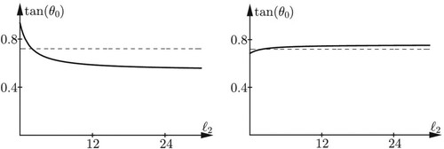In Figure 1, $\tan \left({\theta }_0\right)$ is plotted as a function of ${\ell }_2$ for ${\ell }_1=2$, $h_1=0.7$, and $h_2=1.6$ (left) respectively $h_2=3.4$ (right). The horizontal line is the solution without the bottom layer, given by (23(23) $\tan \left({\theta }_0\right)=\frac{(1+{\ell }_1^2)\sinh \left(2h_1\right)+2{\ell }_1\cosh \left(2h_1\right)+(1-{\ell }_1^2)\sin \left(2h_1\right)}{(1+{\ell }_1^2)\sinh \left(2h_1\right)+2{\ell }_1\cosh \left(2h_1\right)-(1-{\ell }_1^2)\sin \left(2h_1\right)},$(23) ), which of course is independent of ${\ell }_2$. We see that, although the change in $\tan \left({\theta }_0\right)$ due to the presence of the third layer is relatively small, variations in ${\ell }_2$ can lead to both a positive or negative increase of the deflection angle; moreover, the dependence of $\tan \left({\theta }_0\right)$ on ${\ell }_2$ can be considerably changed by choosing different values for $h_2$.

5. Conclusions

We investigated the problem of wind-generated non-equatorial steady ocean currents in the Ekman layer in the case of a piecewise-constant vertical eddy viscosity coefficient with three distinct values in the depth intervals $[-h_1,0]$, $[-h_2,-h_1)$ and $(-\mathrm{\infty },-h_2)$, thereby extending the discussion in [16], where two regions of constant eddy viscosity are considered. We constructed an explicit solution, which enabled us to write down a formula for the surface deflection angle ${\theta }_0$. This formula looks fairly more complicated than in the two-value piecewise-constant case (it depends on four parameters instead of just two), but some considerations on the asymptotic behaviour of ${\theta }_0$ for particular choices of the parameters allow us to say that, unless the top two regions be relatively shallow, ${\theta }_0$ is mostly affected by the depth $h_1$ of the middle layer and the ratio of the values of the eddy viscosity in the top and middle layer, in which case it behaves similarly to the case of just two layers. The corresponding parameters for the bottom layer can have a detectable impact on the deflection angle only if $h_2$ is not too large. Nevertheless, the analysis above suggests that in this case the properties of the deepest layer can affect rather sensibly the deflection angle, both increasing or decreasing its value at the surface. Different combinations of depth and viscosity of this layer can lead to either consequence, highlighting once again the complicated nature of the relation between the eddy viscosity profile and the surface deflection angle. If the middle region becomes very thin, the dynamics will tend again to that of the two-layer case, with the bottom layer playing the main role. Moreover, it turns out that the dependence on the parameters of the bottom layer is not suppressed for a very viscous layer, a feature which is not obvious at first glance.

Figure 1. Plots of $\tan \left({\theta }_0\right)$ as a function of ${\ell }_2$ for ${\ell }_1=2$, $h_1=0.7$, and two different values of $h_2$, namely $h_2=1.6$ (left) and $h_2=3.4$ (right). The dashed horizontal line represents the solution with no bottom layer, formula (23(23) $\tan \left({\theta }_0\right)=\frac{(1+{\ell }_1^2)\sinh \left(2h_1\right)+2{\ell }_1\cosh \left(2h_1\right)+(1-{\ell }_1^2)\sin \left(2h_1\right)}{(1+{\ell }_1^2)\sinh \left(2h_1\right)+2{\ell }_1\cosh \left(2h_1\right)-(1-{\ell }_1^2)\sin \left(2h_1\right)},$(23) ), independent of ${\ell }_2$.

All angles $0<{\theta }_0<{90}^{\circ }$ can be attained in (21(21) $\begin{array}{rl}\tan \left({\theta }_0\right)& =\{{\phi }^2({\alpha }^2-{\text{β}}^2)+{\omega }^2({\gamma }^2-{\delta }^2)+2({\phi }^2+{\omega }^2)(1-{\ell }_1^2)\sin \left(2h_1\right)\\ & +4\left(1-\frac{{\ell }_2^2}{{\ell }_1^2}\right)[\left((1-{\ell }_1^2)\sinh \left(2h_1\right)+(1+{\ell }_1^2)\sin \left(2h_1\right)\right)\cos \left(2\frac{h_2-h_1}{{\ell }_1}\right)\\ & +2{\ell }_1\cos \left(2h_1\right)\sin \left(2\frac{h_2-h_1}{{\ell }_1}\right)]\}\\ & \times \{{\phi }^2({\alpha }^2-{\text{β}}^2)+{\omega }^2({\gamma }^2-{\delta }^2)-2({\phi }^2+{\omega }^2)(1-{\ell }_1^2)\sin \left(2h_1\right)\\ & +4\left(1-\frac{{\ell }_2^2}{{\ell }_1^2}\right)[\left((1-{\ell }_1^2)\sinh \left(2h_1\right)-(1+{\ell }_1^2)\sin \left(2h_1\right)\right)\cos \left(2\frac{h_2-h_1}{{\ell }_1}\right)\\ & -2{\ell }_1\cos \left(2h_1\right)\sin \left(2\frac{h_2-h_1}{{\ell }_1}\right)]{\}}^{-1}.\end{array}$(21) ): If ${\ell }_1\to 0$ and $h_1\to 0$, then $\tan \left({\theta }_0\right)\to \mathrm{\infty }$ or ${\theta }_0\to {90}^{\circ }$, whereas if ${\ell }_1\to \mathrm{\infty }$, $h_2\to \mathrm{\infty }$, and $h_1\to 0$, then $\tan \left({\theta }_0\right)\to 0$ or ${\theta }_0\to 0^{\circ }$. The value ${\theta }_0={45}^{\circ }$ can be attained for all $(h_1,{\ell }_1,h_2,{\ell }_2)$ that satisfy the equation $\begin{array}{rl}& (1-{\ell }_1^2)\sin \left(2h_1\right)\left[\left(1+\frac{{\ell }_2^2}{{\ell }_1^2}\right)\cosh \left(2\frac{h_2-h_1}{{\ell }_1}\right)+2\frac{{\ell }_2}{{\ell }_1}\sinh \left(2\frac{h_2-h_1}{{\ell }_1}\right)\right]\\ & +\left(1-\frac{{\ell }_2^2}{{\ell }_1^2}\right)\left[(1+{\ell }_1^2)\sin \left(2h_1\right)\cos \left(2\frac{h_2-h_1}{{\ell }_1}\right)+2{\ell }_1\cos \left(2h_1\right)\sin \left(2\frac{h_2-h_1}{{\ell }_1}\right)\right]=0,\end{array}$which is derived by setting $\tan \left({\theta }_0\right)=1$.

Acknowledgments

The author would like to thank the anonymous referee for the helpful comments and suggestions.

Data availability

The plots in Figure 1 are easily generated from Equation (21(21) $\begin{array}{rl}\tan \left({\theta }_0\right)& =\{{\phi }^2({\alpha }^2-{\text{β}}^2)+{\omega }^2({\gamma }^2-{\delta }^2)+2({\phi }^2+{\omega }^2)(1-{\ell }_1^2)\sin \left(2h_1\right)\\ & +4\left(1-\frac{{\ell }_2^2}{{\ell }_1^2}\right)[\left((1-{\ell }_1^2)\sinh \left(2h_1\right)+(1+{\ell }_1^2)\sin \left(2h_1\right)\right)\cos \left(2\frac{h_2-h_1}{{\ell }_1}\right)\\ & +2{\ell }_1\cos \left(2h_1\right)\sin \left(2\frac{h_2-h_1}{{\ell }_1}\right)]\}\\ & \times \{{\phi }^2({\alpha }^2-{\text{β}}^2)+{\omega }^2({\gamma }^2-{\delta }^2)-2({\phi }^2+{\omega }^2)(1-{\ell }_1^2)\sin \left(2h_1\right)\\ & +4\left(1-\frac{{\ell }_2^2}{{\ell }_1^2}\right)[\left((1-{\ell }_1^2)\sinh \left(2h_1\right)-(1+{\ell }_1^2)\sin \left(2h_1\right)\right)\cos \left(2\frac{h_2-h_1}{{\ell }_1}\right)\\ & -2{\ell }_1\cos \left(2h_1\right)\sin \left(2\frac{h_2-h_1}{{\ell }_1}\right)]{\}}^{-1}.\end{array}$(21) ).

Disclosure statement

No potential conflict of interest was reported by the authors.

Additional information

Funding

This work was supported by the Vienna Science and Technology Fund (WWTF) under grant MA16-009.

References

- Marshall J, Plumb RA. Atmosphere, ocean and climate dynamics: an introductory text. New York (NY): Academic Press; 2008.
- Constantin A, Johnson RS. The dynamics of waves interacting with the equatorial undercurrent. Geophys Astrophys Fluid Dyn. 2015;109:311–358.
- Ionescu-Kruse D, Martin CI. Periodic equatorial water flows from a Hamiltonian perspective. J Differ Equ. 2017;262:4451–4474.
- Constantin A, Ivanov RI. Equatorial wave-current interactions. Comm Math Phys. 2019;370:1–48.
- Constantin A, Johnson RS. Steady large-scale ocean flows in spherical coordinates. Oceanography. 2018;31:42–50.
- Marynets K. A hyperbolic-type azimuthal velocity model for equatorial currents. Appl Anal. 2019. doi:10.1080/00036811.2020.1774054.
- Marynets K. The modeling of the equatorial undercurrent using the Navier–Stokes equations in rotating spherical coordinates. Appl Anal. 2020. doi:10.1080/00036811.2019.1673375.
- Ekman VW. On the influence of the Earth's rotation on ocean-currents. Ark Mat Astron Fys. 1905;2:1–52.
- Constantin A. Frictional effects in wind-driven ocean currents. Geophys Astro Fluid. 2020;115(1):1–14.
- Yoshikawa Y, Masuda A. Seasonal variations in the speed factor and deflection angle of the wind driven surface flow in the Tsushima Strait. J Geophys Res. 2009;114:C12022.
- Röhrs J, Christensen KH. Drift in the uppermost part of the ocean. Geophys Res Lett. 2015;42:10349–10356.
- Madsen OS. A realistic model of the wind-induced Ekman boundary layer. J Phys Oceanogr. 1977;7:248–255.
- Grisogono B. A generalized Ekman layer profile with gradually varying eddy diffusivities. Quart J Roy Meteorol Soc. 1995;121:445–453.
- Constantin A, Johnson RS. Atmospheric Ekman flows with variable eddy viscosity. Boundary Layer Meteorol. 2019;170:395–414.
- Bressan A, Constantin A. The deflection angle of surface ocean currents from the wind direction. J Geophys Res Oceans. 2019;124:7412–7420.
- Dritschel DG, Paldor N, Constantin A. The Ekman spiral for piecewise-uniform viscosity. Ocean Sci. 2020;16:1089–1093.
- Vallis GK. Atmospheric and oceanic fluid dynamics. 2nd ed. Cambridge (UK): Cambridge University Press; 2017.
- Wuang W, Huang RX. Wind energy input to the Ekman layer. J Phys Oceanogr. 2004;34:1267–1275.
- Cronin MF, Kessler WS. Near-surface shear flow in the tropical Pacific cold tongue front. J Phys Oceanogr. 2009;39:1200–1215.