
 ?Mathematical formulae have been encoded as MathML and are displayed in this HTML version using MathJax in order to improve their display. Uncheck the box to turn MathJax off. This feature requires Javascript. Click on a formula to zoom.
Abstract
Isogeometric analysis is a spline-based discretization method to partial differential equations which show the approximation power of a high-order method. The number of degrees of freedom, however, is as small as the number of degrees of freedom of a low-order method. This does not come for free as the original formulation of isogeometric analysis requires a global geometry function. Since this is too restrictive for many kinds of applications, the domain is usually decomposed into patches, where each patch is parameterized with its own geometry function. In simpler cases, the patches can be combined in a conforming way. However, for non-matching discretizations or for varying coefficients, a non-conforming discretization is desired. An symmetric interior penalty discontinuous Galerkin method for isogeometric analysis has been previously introduced. In the present paper, we give error estimates that are explicit in the spline degree. This opens the door towards the construction and the analysis of fast linear solvers, particularly multigrid solvers for non-conforming multipatch isogeometric analysis.
1. Introduction
The original design goal of isogeometric analysis (IgA) [Citation1] was to unite the world of computer aided design (CAD) and the world of finite element (FEM) simulation. In IgA, both the computational domain and the solution of the partial differential equation are represented by spline functions, like tensor-product B-splines or non-uniform rational B-splines (NURBS). This follows the design goal since such spline functions are also used in standard CAD systems to represent the geometric objects of interest.
The parameterization of the computational domain using just one tensor-product spline function is possible only in simple cases. A necessary condition for this to be possible is that the computational domain is topologically equivalent to the unit square or the unit cube. This might not be the case for more complicated computational domains. Such domains are typically decomposed into subdomains, in IgA called patches, where each of them is parameterized by its own geometry function. The standard approach is to set up a conforming discretization. For a standard Poisson problem, this means that the overall discretization needs to be continuous. For higher order problems, like the biharmonic problem, even more regularity is required, conforming discretizations in this case are rather hard to construct, cf. Ref. [Citation2] and references therein.
Even for the Poisson problem, a conforming discretization requires the discretizations to agree on the interfaces. This excludes many cases of practical interest, like having different grid sizes or different spline degrees on the patches. Since such cases might be of interest, alternatives to conforming discretizations are of interest. One promising alternative is discontinuous Galerkin approaches, cf. Refs. [Citation3, Citation4], particularly the symmetric interior penalty discontinuous Galerkin (SIPG) method [Citation5]. The idea of applying this technique to couple patches in IgA has been previously discussed in Refs. [Citation6–8].
Concerning the approximation error, in early IgA literature, only its dependence on the grid size has been studied, cf. Refs. [Citation1, Citation9]. In recent publications [Citation10–13] also the dependence on the spline degree has been investigated. These error estimates are restricted to the single-patch case. In Ref. [Citation14], the results from Ref. [Citation13] on approximation errors for B-splines of maximum smoothness have been extended to the conforming multipatch case.
For the case of discontinuous Galerkin discretizations, only error estimates in the grid size are known, cf. Ref. [Citation8]. The goal of the present paper is to present an analysis that is explicit both in the grid size h and the spline degree p. We show that the penalty parameter has to grow like for the SIPG method to be well posed. If the solution is sufficiently smooth, the error in the energy norm decays like
. For the analysis of linear solvers, we need also estimates for less smooth functions. We give a bound that degrades only poly-logarithmically with p, cf. (Equation21
(21)
(21) ). These error estimates have recently been used to analyze multigrid solvers for discontinuous Galerkin multipatch discretizations, see Ref. [Citation15]. They might also be helpful for the analysis of Finite Element Tearing and Interconnecting (FETI) solvers, cf. Refs. [Citation6, Citation16], Balancing Domain Decomposition by Constraints (BDDC) solvers, cf. Refs. [Citation17–19] and references therein, Schwarz type solvers, cf. Ref. [Citation20] and references therein, and similar methods.
The remainder of the paper is organized as follows. In Section 2, we introduce the model problem and give a detailed description of its discretization. A discussion of the existence of a unique solution and the discretization and the approximation error is provided in Section 3. The proof of the approximation error estimate is given in Section 4. In Section 5, we provide numerical experiments that depict our estimates. In Section 6, we summarize the findings and discuss possible extensions.
2. The model problem and its discretization
We consider the following Poisson model problem. Let be an open and simply connected Lipschitz domain. For any given source function
, we are interested in the function
solving
(1)
(1) Here and in what follows, for any
,
and
are the standard Lebesgue and Sobolev spaces with standard scalar products
,
, norms
and
, and seminorms
. The Lebesgue space of function with zero mean is given by
.
The computational domain Ω is the union of K non-overlapping open patches , i.e.
(2)
(2) holds, where
denotes the closure of T. Each patch
is represented by a bijective geometry function
which can be continuously extended to the closure of
such that
. We use the notation
for any function v on Ω. If
, we can use standard trace theorems to extend
to
and to extend
to
.
We assume that the mesh induced by the interfaces between the patches does not have any T-junctions, i.e. we assume as follows.
Assumption 2.1
For any two patches and
with
, the intersection
is either (a) empty, (b) a common vertex or (c) a common edge
such that
(3)
(3)
Note that the pre-images and
do not necessarily agree. We define
and
and the parameterization
via
(4)
(4) We assume that the geometry functions agree on the interface (up to the orientation); this does not require any smoothness of the overall geometry function normal to the interface.
Assumption 2.2
For all and
, we have
Remark 2.1
For any domain satisfying Assumption 2.1, we can reparameterize each patch such that this condition is satisfied. Assume to have two patches and
, sharing the patch
. Using
where
we obtain a reparameterization of
, which (a) matches the parameterization of
at the interface, (b) is unchanged on the other interfaces, and (c) keeps the patch
unchanged. By iteratively applying this approach to all patches, we obtain a discretization satisfying Assumption 2.2.
We assume that the geometry function is sufficiently smooth such that the following assumption holds.
Assumption 2.3
There is a constant such that the geometry functions
satisfy the estimates
(5)
(5) for r = 1, 2.
We assume full elliptic regularity.
Assumption 2.4
The solution u of the model problem (Equation1(1)
(1) ) satisfies
for all
.
For domains Ω with a sufficiently smooth boundary, cf. Ref. [Citation21], and for convex polygonal domains Ω, cf. Refs. [Citation22, Citation23], we have and thus also Assumption 2.4. In case of varying diffusion conditions (which are uniform on each patch), we might have
, but Assumption 2.4 might still be satisfied, cf. Refs. [Citation24, Citation25] and others. The theory of this paper can be extended to cases where we only know
for some
. For simplicity, we restrict ourselves to the case of full elliptic regularity, i.e. Assumption 2.4.
Having a representation of the domain, we introduce the isogeometric function space. Following Refs. [Citation7, Citation8], we use a conforming isogeometric discretization for each patch and couple the contributions for the patches using a SIPG method, cf. Ref. [Citation5], as follows.
For the univariate case, the space of spline functions of degree over a grid (vector of breakpoints)
with
and
and size
is given by
where
is the space of polynomials of degree p.
On the parameter domain , we introduce tensor-product B-spline functions
The multipatch function space
is given by
(6)
(6) Note that the grid sizes
and the spline degrees
can be different for each of the patches. We define
to be the largest spline degree, the smallest spline degree, and the grid size. We assume
(7)
(7) for some constant
, where
refers to the smallest knot span.
Following the assumption that is a patchwise function, we define for each
, a broken Sobolev space
with associated norms and scalar products
For each patch, we define on its boundary
, the outer normal vector
. On each interface
, we define the jump operator
by
and the average operator
by
The discretization of the variational problem using the SIPG method reads as follows. Find
such that
(8)
(8) where
for all
, where the penalty parameter
(9)
(9) is chosen sufficiently large.
Using a basis for the space , we obtain a standard matrix-vector problem: find
such that
(10)
(10) Here and in what follows,
is the coefficient vector representing
with respect to the chosen basis, i.e.
, and
is the coefficient vector obtained by testing the right-hand-side functional with the basis functions.
As the dependence on the geometry function is not in the focus of this paper, unspecified constants might depend on ,
, and
. Before we proceed, we introduce a convenient notation.
Definition 2.5
Any generic constant c>0 used within this paper is understood to be independent of the grid size h, the spline degree p, and the number of patches K, but it might depend on the constants ,
, and
.
We use the notation if there is a generic constant c>0 such that
and the notation
if
and
.
For symmetric positive definite matrices A and B, we write
The notations
and
are defined analogously.
3. A discretization error estimate
In Ref. [Citation7], it has been shown that the bilinear form is coercive and bounded in the dG-norm. For our further analysis, it is vital to know these conditions to be satisfied with constants that are independent of the spline degree p. Thus, we define the dG-norm via
(11)
(11) for all
. Note that we define the norm differently to Ref. [Citation7], where the dG-norm was independent of p.
Before we proceed, we give some estimates on the geometry functions.
Lemma 3.1
We have
(12)
(12) where r = 0, 1, 2. For ease of notation, here and in what follows, we define
. If (Equation5
(5)
(5) ) holds for
with some s>r, then (Equation12
(12)
(12) ) also holds for those choices of r. Moreover, we have
Proof.
The statements follow directly from the chain rule for differentiation, the substitution rule for integration, and Assumption 2.3.
Lemma 3.2
We have for all
.
Proof.
We have where certainly
because the length of
is always 1. The estimate
follows directly from the chain rule for differentiation, the substitution rule for integration, and Assumption 2.3.
For σ sufficiently large, the symmetric bilinear form is coercive and bounded, i.e. a scalar product.
Theorem 3.3
Coercivity and boundedness
There is some that only depends on
,
, and
such that
hold for all
and all
.
Proof.
Note that Using Lemma 3.2, [Citation14, Lemma 4.4], [Citation26, Corollary 3.94], and Lemma 3.1, we obtain
(13)
(13) for all
,
, and
. As
, the Poincaré inequality (see, e.g. Ref. [Citation26, Theorem A.25]) yields also
The Cauchy–Schwarz inequality, the triangle inequality, (Equation13
(13)
(13) ), and
yield
(14)
(14) for all
. Let
be the hidden constant, i.e. such that
(15)
(15) For
, we obtain
i.e. coercivity. Using (Equation14
(14)
(14) ) and the Cauchy–Schwarz inequality, we obtain further
i.e. boundedness.
As we have boundedness and coercivity (Theorem 3.3), the Lax Milgram theorem (see, e.g. Ref. [Citation26, Theorem 1.24]) yields states existence and uniqueness of a solution, i.e. the following statement.
Theorem 3.4
Existence and uniqueness
If σ is chosen as in Theorem 3.3, the problem (Equation8(8)
(8) ) has exactly one solution
.
The following theorem shows that the solution of the original problem also satisfies the discretized bilinear form.
Theorem 3.5
Consistency
The solution of the original problem (Equation1
(1)
(1) ) satisfies
For a proof, see, e.g. Ref. [Citation4, Proposition 2.9]; the proof requires elliptic regularity (cf. Assumption 2.4).
If boundedness of the bilinear form was also satisfied for
, Ceá's Lemma (see, e.g. Ref. [Citation26, Theorem 2.19.iii]) would allow to bound the discretization error. However, the bilinear form is not bounded in the norm
, but only in the stronger norm
, given by
(16)
(16)
Theorem 3.6
If σ is chosen as in Theorem 3.3,
holds for all
and all
.
Proof.
Let and
be arbitrarily but fixed. Note that the arguments from (Equation14
(14)
(14) ) also hold if the first parameter of the bilinear form
is not in
. So, we obtain
Using Lemma 3.2, [Citation14, Lemma 4.4], Lemma 3.1, and the Poincaré inequality, we obtain
(17)
(17) for all
, all
, all
, and all
. Using this estimate, and
, we obtain for
Using these estimates, we obtain
which finishes the proof.
Using consistency (Theorem 3.5), coercivity, and boundedness (Theorems 3.3 and 3.6), we can bound the discretization error using the approximation error.
Theorem 3.7
Discretization error estimate
Provided the assumptions of Theorems 3.3 and 3.5, the estimate
holds, where u is the solution of the original problem (Equation1
(1)
(1) ) and
is the solution of the discrete problem (Equation8
(8)
(8) ).
Proof.
For any , the triangle inequality yields
(18)
(18) Theorem 3.5 and Galerkin orthogonality yield
for all
. So, we obtain using Theorems 3.3 and 3.6 that
which shows
. Together with (Equation18
(18)
(18) ), this shows
. Since this holds for all
, this finishes the proof.
Theorem 3.8
Approximation error estimate
Let . Provided that σ is as in Theorem 3.3 and that
for
(cf. Lemma 3.1), then
(19)
(19) holds for all
.
A proof of this theorem is given at the end of the next section.
Assuming , then we have for the case
that
For the analysis of linear solvers, like multigrid solvers [Citation15], we also need low-order approximation error estimates. In the convergence proofs, we usually have to estimate errors of the iterative scheme. Even if we know that the true solution satisfies certain regularity assumptions, this does not extend to the errors. For them, we can only rely on the regularity statements arising from the domain, which means that
-regularity is usually the best we can hope for. For this case, we obtain
This means that we obtain a quadratic increase in the spline degree p. Using a refined analysis, we obtain as follows.
Theorem 3.9
Low-order approximation error estimate
Provided that σ is as in Theorem 3.3, then the estimate
(20)
(20) holds for all
.
The proof is given at the end of the next section. Assuming again , we obtain
(21)
(21) i.e. an only poly-logarithmic increase in the spline degree p.
4. Proof of the approximation error estimates
Before we can give the proof, we give some auxiliary results. This section is organized as follows. In Section 4.1, we give patchwise projectors and estimates for them. We introduce a mollifying operator and give estimates for that operator in Section 4.2. Finally, in Section 4.3, we give the proof for the approximation error estimate.
4.1. Patchwise projectors
As first step, we recall the projection operators from Ref. [Citation14, Sections 3.1 and 3.2]. Let be the
-orthogonal projection into
, where
In what follows, we also write
and
if we refer to a uniform grid of size h. Takacs [Citation14, Lemma 3.1] states that
and
. Using
, we obtain for
and
that
(22)
(22) The next step is to consider the multivariate case, more precisely the parameter domain
. Let
and
be given by
and let
be such that
(23)
(23) For the physical domain, define
to be such that
Observe that we obtain using (Equation22
(22)
(22) ) that
(24)
(24) for all
.
The projectors satisfy robust error estimates and are almost stable in
.
Lemma 4.1
Let Z be a grid of size h, , and
. Then,
hold for all
.
Proof.
The identity (Equation22(22)
(22) ) implies that the projector
coincides with the projector
from Ref. [Citation12, Equations (3.8) and (3.9)]. Thus, the desired result follows from Ref. [Citation12, Theorem 3.1].
Lemma 4.2
Let Z be a quasi-uniform grid of size h, , and
. Then,
holds for all
.
Proof.
The proof is analogous to the proof of Ref. [Citation27, Theorem 4]. Let be the
-orthogonal projector into
as introduced in Ref. [Citation12]. Using the triangle inequality and a standard inverse estimate [Citation26, Corollary 3.94], we obtain
Thus, the desired result follows from Ref. [Citation12, Theorem 3.1].
Lemma 4.3
Let . The estimates
hold for all
.
Proof.
The proof is based on the univariate estimates given in Lemmas 4.1 and 4.2 ( and the quasi-uniformity of the grids have been required in (Equation7
(7)
(7) )) and follows the standard construction that can be found, e.g. in the proof of Ref. [Citation14, Theorem 3.3].
On the interfaces, we have the following approximation error estimate.
Lemma 4.4
Let and
. Then, the estimate
holds for all
.
Proof.
Without loss of generality, we assume . Because of Ref. [Citation14, Theorem 3.4], we know that
. So, we have
Using Refs. [Citation14, Equation (3.4)], [Citation28, Lemma 8] and that
minimizes the
-seminorm, we further obtain
Sande et al. [Citation12, Theorem 3.1] provide the desired result.
4.2. A mollifying operator
A second step of the proof is the introduction of a particular mollification operator for the interfaces.
For , let
be given by
. For
, we define
, i.e. we have
or
, cf. Assumption 2.2. For all cases,
is a bijective function
and
(25)
(25) holds for all s. For
, we define the abbreviated notation
and observe
For
, we define extension operators
by
where
(26)
(26) Now, define for each patch
, a mollifying operator
by
(27)
(27) The combination of the patch local operators yields a global operator
:
(28)
(28) Observe that
preserves constants, i.e.
(29)
(29)
Lemma 4.5
For all and all
, we have
Proof.
Assume without loss of generality that . For this case, we have
As
, we obtain
. This shows the first statement for the two boundary segments adjacent to
, i.e.
and
. Since
yields
, we also have the first statement for the boundary segment
. This finishes the proof for the first statement. The proof for the second statement follows directly from
.
Lemma 4.6
holds for all
.
Proof.
Equation (Equation27(27)
(27) ) implies
. Observe that the projector
is interpolatory on the boundary [Citation14, Lemma 3.1]. So,
maps into
and
maps into
. Therefore, Lemma 4.5 yields
, which immediately implies the desired result.
Before we proceed, we give a certain trace like estimate.
Lemma 4.7
The estimate
holds for all
and
and all
.
Proof.
A trace theorem [Citation14, Lemma 4.4] yields
(30)
(30) Case 1. Assume
. In this case, we choose v to be the
-orthogonal projection of u into
. Since the spline degree of that space is fixed, we obtain using a standard inverse inequality [Citation26, Corollary 3.94] and a standard approximation error estimate (like from Ref. [Citation13]) that
Case 2. Assume
. In this case, we choose
and obtain from (Equation30
(30)
(30) ) directly
In this case, the Poincaré inequality finishes the proof.
As a next step, we show that the mollifier constructs functions that are very smooth on the interfaces.
Lemma 4.8
The estimate holds for all
and all
.
Proof.
We have using (Equation25(25)
(25) ) and Lemma 4.6
Now, a standard inverse estimate [Citation26, Corollary 3.94] yields
where
. Lemma 4.2 and the
-stability of
yield
so we obtain
Using (Equation25
(25)
(25) ), we obtain
By applying Lemma 4.7 to the derivative of
, we obtain the desired result.
Lemma 4.9
holds for all
and
.
Proof.
Let be arbitrary but fixed.
We obtain using the definition of and
and Lemma 3.1 that
(31)
(31) holds, where
and
. Since
, a standard trace theorem yields
(32)
(32) Thus, (Equation31
(31)
(31) ) implies
. By plugging
into (Equation31
(31)
(31) ), we obtain using Lemma 4.6
Using (Equation32
(32)
(32) ) and
, we obtain
and consequently also
.
Lemma 4.10
The estimate holds for all
and
.
Proof.
Using the definition of and of the
-norm, we obtain
(33)
(33) where
for
and
We estimate the terms
,
, and
separately. Let without loss of generality
.
Step 1. Using (Equation23(23)
(23) ) and the
-stability of the
-orthogonal projection, and
, we obtain
where we use
. The triangle inequality yields
Lemma 4.1 yields
The definition of w and (Equation25
(25)
(25) ) yield
Lemma 4.1 yields
Equation (Equation25
(25)
(25) ) yields further
Now, Lemma 4.7 applied to the derivative of u yields
(34)
(34) Step 2. Using (Equation23
(23)
(23) ) and the
-stability of the
-orthogonal projection and
, we obtain
Using
and the definition of w, we obtain
Using (Equation25
(25)
(25) ), we obtain further
Using the
-stability of
and the approximation error estimate [Citation14, Theorem 3.1], we obtain
Using (Equation25
(25)
(25) ) and Lemma 4.7 applied to the derivative of
, we obtain
(35)
(35) Step 3. Using
and (Equation22
(22)
(22) ), we obtain
Using (Equation34
(34)
(34) ), and using
, we further obtain
(36)
(36) Concluding step. The combination of (Equation33
(33)
(33) )–(Equation36
(36)
(36) ) yields the desired result.
4.3. The approximation error estimate
The following three lemmas give approximation error estimates (Equation20(20)
(20) ) for the choice
separately for the individual parts of
.
Lemma 4.11
holds for all
.
Proof.
First note that the Poincaré inequality yields
(37)
(37) Let
be arbitrary but fixed and let
. Using Lemma 3.1, the triangle inequality, (Equation37
(37)
(37) ), and (Equation24
(24)
(24) ), we obtain
We further obtain using Lemmas 4.3 and 4.10,
Lemma 3.1, (Equation24
(24)
(24) ), (Equation29
(29)
(29) ), and the Poincaré inequality finish the proof.
Lemma 4.12
holds for all
.
Proof.
Using Lemma 3.1, the triangle inequality, (Equation37(37)
(37) ), (Equation24
(24)
(24) ), and a standard inverse inequality ([Citation26, Corollary 3.94]), we obtain
By again applying Lemmas 4.3 and 4.10, we obtain
Lemma 3.1, (Equation24
(24)
(24) ), (Equation29
(29)
(29) ) and the Poincaré inequality finish the proof.
Lemma 4.13
holds for all
.
Proof.
Let be arbitrary but fixed and let
. Observe that the triangle inequality, Lemmas 4.9 and 3.1 yield
Lemma 4.4 yields
Since Assumption 2.2 yields
, we obtain
and therefore also
Now, Lemma 4.8 yields
Lemma 3.1 finishes the proof.
Finally, we can show Theorems 3.8 and 3.9.
Proof of Theorem 3.9.
Proof of Theorem 3.9.
Let be arbitrary but fixed and define
.
First, we show that
(38)
(38) holds for any
and all
.
Case 1. Assume . In this case, we define
and observe
Equation (Equation16
(16)
(16) ), Lemmas 4.11–4.13, and
yield
and since
further (Equation38
(38)
(38) ).
Case 2. Assume . Define
i.e. the set of all globally continuous functions which are locally just linear. Observe that
. Using u and w being continuous, we obtain
For the choice
where
we further obtain using standard approximation error estimates and Lemma 3.1
where
. Using
,
, and
, we have
which shows (Equation38
(38)
(38) ) also for the second case.
Finally, we show that Ψ is such that the desired bound (Equation20(20)
(20) ) follows. We again consider two cases.
Case 1. Assume . In this case, we choose
where
is Euler's number (
), and obtain
which finishes the proof for Case 1.
Case 2. Assume . In this case, we choose
and obtain immediately
which finishes the proof for Case 2.
Proof of Theorem 3.8.
Proof of Theorem 3.8.
Let be arbitrary but fixed and define
. The definition of the
-norm and the
-norm yield
Using the triangle inequality and Lemma 3.1, we have further
where
. Using a trace theorem [Citation14, Lemma 4.4] and
, we obtain
Using this,
, and
, we obtain
The desired result is then a consequence of Lemma 4.3 and the assumed equivalence of the norms on the physical domain and the parameter domain.
5. Numerical experiments
We depict the results of this paper with numerical results.
For the first experiments, we choose a spline approximation of the quarter annulus . This domain is uniformly split into
patches in the obvious way. We solve the Poisson equation
where
is the exact solution. On each patch, we introduce a coarse discretization space
for
, which only consists of global polynomials of degree p. We then refine all grids
times uniformly. Next, we modify the discretization spaces in order to obtain non-matching discretizations at the interfaces (since fully matching discretizations would be a special case that would allow a conforming discretization that would not be of interest in a discontinuous Galerkin setting): we refine the grid one additional time for one-third of the patches and we increase the spline degree to p + 1 for another third of the patches.
In Table and Figures and , we depict the discretization errors in the
-norm relative to that of the solution and the rates
, given by
for the case that the smoothness is
on the patches with spline degree p and
on the patches with spline degree p + 1 (maximum smoothness). The numerical experiments show that the error decreases like
or even faster. Whether or not the error bound depends on
or
cannot be seen in this experiment. The almost p-robust convergence of multigrid solvers whose analysis follows from the presented results can be seen in Ref. [Citation15].
Figure 1. Discretization errors for splines of maximum smoothness as function in ℓ.
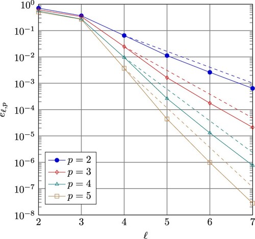
Figure 2. Discretization errors for splines of maximum smoothness as function in p.
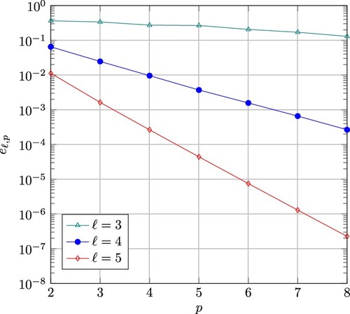
Table 1. Discretization errors in case of maximum smoothness.
In Table and Figure , we choose smoothness on all patches (minimum smoothness). The grid sizes and the degrees are chosen as for the first experiment. The configurations for which the computation could not be completed due to a lack of memory are indicated by ‘OoM '. We obtain qualitatively the same behavior as for splines of maximum smoothness. We observe that the number of degrees of freedom in case of minimum smoothness is much larger than in the case of minimum smoothness, which outweighs the fact that for the minimally smooth approximation, slightly smaller errors are obtained.
Figure 3. Discretization errors for splines of minimum smoothness as function in ℓ.
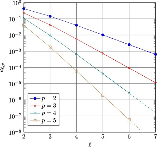
Table 2. Discretization errors in case of minimum smoothness.
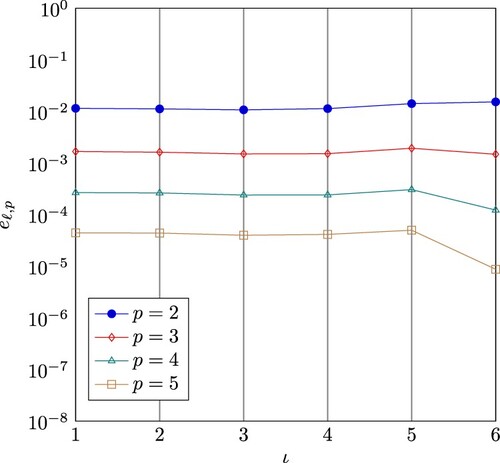
In Figure , one can observe the dependence of the discretization error on the number of patches. Here, we consider a decomposition of the initial domain into patches, where
. We again consider a heterogeneous discretization (different spline degrees, different grid sizes), where we apply
uniform refinement steps. So, the grid sizes are constant. We observe that also the discretization errors are rather constant.
Figure 4. Errors for splines of maximum smoothness with patches and
.
Finally, we present an experiment that goes beyond the presented theory. Here, we consider the Fichera corner as computational domain. This domain is composed of the patches ,
,
, and
. Each of the patches is parameterized with the appropriately shifted identity function. We solve
(39)
(39) where
is the exact solution. We choose
on the patch
and
on the remaining patches. The SIPG formulation reads as follows. Find
such that
(40)
(40) holds for all
, where
(41)
(41) The discretization spaces on the patches are obtained by
uniform refinement steps, where we use splines of maximum smoothness with degree p + 1 on the patch
and with degree p on the remaining patches. This means that, again, for each interface, the intersection of the traces of the local function spaces of the involved spaces only contains global polynomials, so this is again a non-conforming discretization. We present the corresponding results in Table . As for the first experiment, we obtain the convergence rates that are slightly better than the expected ones.
Table 3. Discretization errors in case of maximum smoothness in 3D.
6. Conclusions and possible extensions
In this paper, we have introduced an SIPG discretization of the Poisson equation in two dimensions which is well posed in the dG-norm, see Theorem 3.3. We have seen that the well-posedness is robust in the grid size and the spline degree. The approximation error estimate presented in Theorem 3.8 shows that the proposed method satisfies the expected approximation order. The approximation error estimate presented in Theorem 3.9 gives an error estimate in the -norm, which only grows logarithmically in the spline degree and which is of particular interest for the analysis of iterative solvers.
Remark 6.1
Splines of reduced smoothness
The proofs of Theorems 3.3 and 3.6 (coercivity and boundedness) do not use that the considered spline space is of maximum smoothness. Thus, Theorems 3.4 (existence and uniqueness), 3.5 ( consistency), and 3.7 (discretization error estimate) also apply if splines of reduced smoothness are used. Since the space of splines of maximum smoothness forms a subspace of the spaces of splines of reduced smoothness, the approximation error estimates given in Theorems 3.8 and 3.9 are also valid for spline spaces of reduced smoothness.
Remark 6.2
Three-dimensional domains
The extension of the proposed discretization technique to three-dimensional domains is completely straight-forward. Here, the interfaces are two-dimensional faces between patches, so the set
contains the indices of patches that share such faces. The proofs of Lemmas 3.1 and 3.2 and Theorems 3.3 and 3.6 (coercivity and boundedness) apply almost verbatim also to three-dimensional domains. Thus, Theorems 3.4 (existence and uniqueness), 3.5 ( consistency), and 3.7 (discretization error estimate) apply as well. The extension of the approximation error estimates to three dimensions is more involved since the extension of (Equation23
(23)
(23) ) to
yields a projector that is well defined only in
. Based on this observation, Theorem 3.8 (approximation error estimate) can be extended to three dimensions, provided that
. For the extension of Theorem 3.8 (low-order approximation error estimate), one would need to construct an
-stable projectors and appropriate mollifiers, which goes beyond the scope of this paper.
Remark 6.3
Other differential equations
The theory presented in this paper can be extended to other elliptic differential equations whose variational formulation lives in the Sobolev space . If the differential equation is parameter-dependent, like (Equation39
(39)
(39) ), a parameter-dependent SIPG formulation can be introduced, cf. (Equation40
(40)
(40) )–(Equation41
(41)
(41) ). For the problem (Equation40
(40)
(40) )–(Equation41
(41)
(41) ), analogous versions to Theorems 3.3 and 3.6 ( coercivity and boundedness) can be shown for the corresponding parameter-dependent dG-norms, i.e. the norms are given by the combination of (Equation11
(11)
(11) ), (Equation16
(16)
(16) ), and (Equation41
(41)
(41) ). Thus, Theorems 3.4 (existence and uniqueness), 3.5 ( consistency), and 3.7 (discretization error estimate) apply as well. Approximation error estimates analogous to Theorems 3.8 ( approximation error estimate) and Theorem 3.8 (low-order approximation error estimate) hold, where the constants depend on
and the
-norms are parameter-dependent norms as defined in (Equation41
(41)
(41) ).
Disclosure statement
No potential conflict of interest was reported by the author.
Additional information
Funding
References
- Hughes TJR, Cottrell JA, Bazilevs Y. Isogeometric analysis: CAD, finite elements, NURBS, exact geometry and mesh refinement. Comput Methods Appl Mech Eng. 2005;194(39–41):4135–4195.
- Kapl M, Sangalli G, Takacs T. Isogeometric analysis with C1 functions on unstructured quadrilateral meshes. SMAI J Comput Math. 2019;S5:67–86.
- Arnold D, Brezzi F, Cockburn B, et al. Unified analysis of discontinuous Galerkin methods for elliptic problems. SIAM J Numer Anal. 2002;39(5):1749–1779.
- Rivière B. Discontinuous Galerkin methods for solving elliptic and parabolic equations. Philadelphia: Society for Industrial and Applied Mathematics; 2008.
- Arnold D. An interior penalty finite element method with discontinuous elements. SIAM J Numer Anal. 1982;19(4):742–760.
- Hofer C, Langer U. Dual-primal isogeometric tearing and interconnecting solvers for multipatch dG-IgA equations. Comput Methods Appl Mech Eng. 2017;316:2–21.
- Langer U, Mantzaflaris A, Moore S, et al. Multipatch discontinuous Galerkin isogeometric analysis. In: Jüttler B, and Simeon B, editors. Isogeometric analysis and applications. Cham: Springer; 2015. p. 1–32.
- Langer U, Toulopoulos I. Analysis of multipatch discontinuous Galerkin IgA approximations to elliptic boundary value problems. Comput Vis Sci. 2015;17(5):217–233.
- Bazilevs Y, Beirão da Veiga L, Cottrell JA, et al. Isogeometric analysis: approximation, stability and error estimates for h-refined meshes. Math Models Methods Appl Sci. 2011;16(7):1031–1090.
- Beirão da Veiga L, Buffa A, Rivas J, et al. Some estimates for h–p–k-refinement in isogeometric analysis. Numer Math. 2011;118(2):271–305.
- Floater M, Sande E. Optimal spline spaces of higher degree for L2 n-widths. J Approx Theor. 2017;216:1–15.
- Sande E, Manni C, Speleers H. Sharp error estimates for spline approximation: explicit constants, n-widths, and eigenfunction convergence. Math Models Methods Appl Sci. 2019;29(6):1175–1205.
- Takacs S, Takacs T. Approximation error estimates and inverse inequalities for B-splines of maximum smoothness. Math Models Methods Appl Sci. 2016;26(7):1411–1445.
- Takacs S. Robust approximation error estimates and multigrid solvers for isogeometric multi-patch discretizations. Math Models Methods Appl Sci. 2018;28(10):1899–1928.
- Takacs S. Fast multigrid solvers for conforming and non-conforming multi-patch isogeometric analysis. Comput Methods Appl Mech Eng. 2020;371:113301.
- Schneckenleitner R, Takacs S. Convergence theory for IETI-DP solvers for discontinuous Galerkin Isogeometric Analysis that is explicit in h and p. Comput Meth Appl Math. 2021. DOI:10.1515/cmam-2020-0164.
- Beirão da Veiga L, Cho D, Pavarino L, et al. BDDC preconditioners for isogeometric analysis. Math Models Methods Appl Sci. 2013;23(6):1099–1142.
- Beirão da Veiga L, Pavarino L, Scacchi S, et al. Adaptive selection of primal constraints for isogeometric BDDC deluxe preconditioners. SIAM J Sci Comput. 2017;39(1):A281–A302.
- Canuto C, Pavarino L, Pieri A. BDDC preconditioners for continuous and discontinuous Galerkin methods using spectral/hp elements with variable local polynomial degree. IMA J Numer Anal. 2014;34(3):879–903.
- Beirão da Veiga L, Cho D, Pavarino L, et al. Overlapping Schwarz methods for isogeometric analysis. SIAM J Numer Anal. 2012;50(3):1394–1416.
- Necas J. Les méthodes directes en théorie des équations elliptiques. Paris: Masson; 1967.
- Dauge M. Elliptic boundary value problems on corner domains. Smoothness and asymptotics of solutions. Berlin: Springer; 1988 (Lecture Notes in Mathematics; 1341).
- Dauge M. Neumann and mixed problems on curvilinear polyhedra. Integr Equ Oper Theor. 1992;15:227–261.
- Petzoldt M. Regularity and error estimators for elliptic problems with discontinuous coefficients [Ph.D. thesis]. Berlin: Freie Universität Berlin, Weierstraß–Institut für Angewandte Analysis und Stochastik; 2001.
- Petzoldt M. A posteriori error estimators for elliptic equations with discontinuous coefficients. Adv Comput Math. 2002;16(1):47–75.
- Schwab C. p- and hp-finite element methods: theory and applications in solid and fluid mechanics. Oxford: Clarendon Press; 1998 (Numerical Mathematics and Scientific Computation).
- Hofreither C, Takacs S. Robust multigrid for isogeometric analysis based on stable splittings of spline spaces. SIAM J Numer Anal. 2017;55(4):2004–2024.
- Hofreither C, Takacs S, Zulehner W. A robust multigrid method for isogeometric analysis in two dimensions using boundary correction. Comput Methods Appl Mech Eng. 2017;316:22–42.