Resonance frequencies of arbitrarily shaped dielectric cylinders

ABSTRACT

We consider eigenvalue problems for dielectric cylindrical scatterers of arbitrary cross with generalized conditions at infinity that enable one to take into account complex eigenvalues. The existence of resonance (scattering) frequencies associated with these eigenvalues is proved. The technique involves the determination of characteristic numbers (CNs) of the Fredholm operator-valued functions of the problems constructed using Green's potentials. Separating principal parts in the form of meromorphic operator pencils, we apply the operator generalization of Rouché's theorem to verify the occurrence of CNs in close proximities of the pencil poles. The results are illustrated in detail using the case of a dielectric cylinder of circular cross section.

KEYWORDS:

• Resonance frequencies
• boundary integral equations
• operator-valued functions
• finite-meromorphic
• pole pencils

2020 MATHEMATICS SUBJECT CLASSIFICATIONS:

• 35B34
• 45B05
• 45C05
• 45E99
• 47A10

1. Introduction

Analysis of fundamental (scattering), or resonance, frequencies (RFs) constitutes one of central topics of mathematical physics [1,2], electromagnetics [3,4], and acoustics [6], and is a core subject of the spectral theory of open structures [4]. The verification of the existence and analysis of the RF distribution on the complex plane are key issues for open structures: resonators, waveguides, and transmission lines. Apart from the knowledge of eigenvalues of the corresponding nonselfadjoint boundary eigenvalue problems (BEPs) in open domains, which is important by itself, the information about the location of RFs enables researchers to investigate resonance scattering and solve inverse problems of identifying parameters of the inclusions. In fact, abrupt increase of the scattered field takes place when the (real) frequency of the exciting field (e.g. a plane wave) falls into the close proximity of the real part of a (complex) RF. Thus the knowledge of RFs allows, on the one hand, to predict the resonance behavior of the scatterer, and, on the other hand, to associate resonance peaks with irregularities of the boundary or inclusions which opens the way to the solution of the corresponding inverse problems. Such resonance effects were exemplified in many studies, e.g. in [5] for a cavity-backed slotted screen.

For several canonical coordinate domains forming the cross-section of a cylindrical scatterer like a circle and an ellipse, finding RFs can be reduced, using separation of variables in cylindrical coordinates [7–9], to the determination of complex zeros of functions of one complex variable and several real or complex parameters [10]. However, even for a dielectric cylinder of circular shape, a dielectric rod (DR), a rigorous proof of the RF existence has been an open question. Only recently this problem has been solved in [12] where it has been shown that the RF determination can be reduced to finding zeros of a family of weighted cross-products of cylindrical functions. The latter have been referred to as generalized cylindrical polynomials (GCPs) in [13] where the elements of the GCP theory have been elaborated that enable one to determine the occurrence and location of zeros.

In [4,5,11,14], and [15], the existence of RFs was demonstrated for certain families of shielded and open metal-dielectric scatterers formed in the cross section by (bounded) domains (particularly, in [11] for the union or rectangular domains with slots on the common part of the boundary) and ‘slotted’ open domains (a cavity-backed slotted screen in [5]). However, these results have never been extended to the case when the boundary curve of a cylindrical dielectric scatterer is a single arbitrary smooth (or piecewise smooth) simply-connected contour. For such structures, the methods of boundary integral equations (BIEs) developed in [16] and [17] (see comprehensive lists of references therein reflecting the state-of-the-art) and summation equations [4,18] have been a subject of intense studies. A characteristic feature (and a drawback) of the BIE method as applied to the calculation of complex eigenvalues for dielectric scatterers in open domains is the absence of preliminary information about the existence and location of the sought eigenvalue spectrum. This is one of the main reasons to accomplish the present study; an objective is, apart from the theoretical findings and novelty, to complement the BIE method with a tool to perform justified and efficient computations of RFs.

It should be noted that the results of this work may definitely help in the analysis of fictitious eigenvalues identified in [17] as well as anomalous resonance scattering and singularities [5,20] of the diffracted fields.

Spectral theory of operator-valued functions (OVFs) and operator pencils (OPs) with a nonlinear dependence on the spectral parameter relevant to our studies was developed mainly by Gohberg and his co-workers starting from the early 1950s and was summarized then in a great number of monographs including [21,22]. The beginning of application of this theory to the analysis of oscillations, waves, and resonance scattering in electromagnetics and acoustics dates back to the late 1970s when the pioneering works [23–28] were published. A characteristic feature of the approach is introduction of a correct statement, for the first time in [19], of a boundary eigenvalue problem for the RF determination with the generalized Sveshnikov–Reichardt conditions at infinity that enable one to handle complex eigenvalues (RFs) of open structures. The findings were summarized then in monographs [4,27] and [14]. In the continuation, the studies addressed [29] wave propagation in transmission lines of various types. Substantiation of the method of generalized potentials [31,32] (included then to [14] and [4]) gave rise to elaborating an approach that employs layer-potential boundary integral operators and BIEs and further development of the spectral theory for electromagnetics [32–35]. The latter involves integral OVFs with a logarithmic singularity of the kernel [14], in particular finite-meromorphic integral OPs (IOPs) associated with the determination of RFs of open two-dimensional (cylindrical) resonators. For the first time, finite-meromorphic OVFs and IOPs were applied for the analysis of resonance scattering in [28,29]; a consistent presentation of the method was performed later in [4] and [14] where, among all, explicit formulas for the IOP characteristic numbers (CNs) were obtained. Comprehensive asymptotic analysis and explicit formulas for RFs of narrow-slot scatterers (as segments of small-parameter series) are presented in [4] and [14]. The study was extended in [5,11] where particularly multi-slot and multi-strip scatterers were considered, both shielded and open.

Methods of the OVF spectral theory in combination with the layer BIEs and IOPs were extensively applied in a series of papers among which we note [37] and were summarized then in the monograph [38]. It should be noted however that a priority here is connected with the results obtained (a decade earlier) in our studies which led to the construction in the 1990s of a unified approach called the spectral theory of open structures [4]. It seems that the authors of [38] were not aware of these findings; in any case, they never cited them in their works published after 1998. We note that, actually, our achievements and the techniques and results of H. Ammari and coworkers complement each other in many aspects. Particularly, we paid a considerable attention to the determination of CNs of logarithmic integral operators on one or several integration intervals (in planar [5,11,14,15] and circular [39] domains) using asymptotic semi-inversion and performing, in [5,14,20] and several other works, detailed studies of small-parameter series.

The existence of RFs is an urgent issue in the theory of transmission eigenvalues (TEs) [41]. The technique proposed in this work may contribute to the progress in the TE studies and in particular to finding intersections of the TE and RF sets for certain classes of scatterers.

This study may be considered as part of a broad framework of the BIE applications to the analysis of RFs in open dielectric structures and beyond. Several works were published in SIAM journals on this topic, including papers [16] and [17] (one may also refer to the references therein). The present paper is aimed to fill the existing gap in the BIE theory providing validation of the RF determination using numerical methods.

The paper is organized as follows. In Section 2, the statement of the RF problem is formulated. In Sections 3 and 4, Green's functions and Green's potentials are introduced and the properties of integral operators with a logarithmic singularity on closed contours are presented. In Section 5, the RF boundary eigenvalue problem is reduced to the determination of characteristic numbers (CNs) of a finite-meromorphic integral operator-valued function (OVF). A central result of the study is in Section 6 where the existence of CNs of the OVF derived in Section 5 and the RFs is proved. The principal OVF singular parts in the form of pole pencils are separated and the pole-pencil CNs (approximations to the sought RFs) are obtained as well as formulas for the CN calculation using in particular Fourier expansions. Section 7 is devoted to a detailed analysis of an example of application when the boundary contour is a circle. The paper ends with a conclusion and an appendix, which provides specific calculation results.

2. Statement of the problem on resonance frequencies

Let Γ be a closed smooth curve in the two-dimensional space $R^2$ dividing it into two domains, a bounded ${\mathrm{\Omega }}_{{ϵ}_1}$, and an unbounded ${\mathrm{\Omega }}_{{ϵ}_2}$. Following [4], Chapter 1, and [16] formulate the problem of determining RFs (eigenoscillations) of a dielectric cylinder as a T eigenvalue problem (TEP) for the Helmholtz equation with the generalized outgoing Sveshnikov–Reichardt conditions at infinity (1) $\begin{array}{rl}\mathrm{\Delta }u(\mathbf{x})+k^2ϵu(\mathbf{x})& =0,\mathbf{x}\in {\mathrm{R}}^2\setminus \mathrm{\Gamma },\end{array}$(1) (2) $\begin{array}{rl}{\left[u\right]|}_{\mathrm{\Gamma }}& =0,\end{array}$(2) (3) $\begin{array}{rl}{\left[\frac{\mathrm{\partial }u}{\mathrm{\partial }n}\right]|}_{\mathrm{\Gamma }}& =0(\mathrm{E}-\mathrm{oscillations}),\mathrm{or}\end{array}$(3) (4) $\begin{array}{rl}{\left[\frac{1}{ϵ}\frac{\mathrm{\partial }u}{\mathrm{\partial }n}\right]|}_{\mathrm{\Gamma }}& =0(\mathrm{H}-\mathrm{oscillations}),\end{array}$(4) (5) $\begin{array}{rl}u(\mathbf{x})& =\sum _{m=-\mathrm{\infty }}^{\mathrm{\infty }}{a}_m{H}_m^{(1)}(k\sqrt{{ϵ}_2}r)e^{im\varphi },r\ge R_0,\mathbf{x}=(r,\varphi );\end{array}$(5) here $H_m^{(1)}(z)$ are the mth-order first-kind Hankel functions; $R_0$ is the radius of a circle $B_{R_0}$ centered at the origin such that ${\mathrm{\Omega }}_{{ϵ}_1}\subset B_{R_0}$; [] denotes the difference of the limiting values of the functions from inside and outside with respect to (w.r.t.) domain ${\mathrm{\Omega }}_{{ϵ}_1}$ bounded by Γ; $ϵ=ϵ(\mathbf{x})={ϵ}_j$, $\mathbf{x}\in {\mathrm{\Omega }}_{{ϵ}_j}$, j = 1, 2, is a piecewise constant quantity (real or complex) specifying permittivity of the domains; $\frac{\mathrm{\partial }}{\mathrm{\partial }n}$ is the directional derivative with respect to the external unit normal vector to Γ; series (5(5) $\begin{array}{rl}u(\mathbf{x})& =\sum _{m=-\mathrm{\infty }}^{\mathrm{\infty }}{a}_m{H}_m^{(1)}(k\sqrt{{ϵ}_2}r)e^{im\varphi },r\ge R_0,\mathbf{x}=(r,\varphi );\end{array}$(5) ) is absolutely and uniformly convergent in every ring $a\le r\le b$, $b>a>R_0$, and admits double termwise differentiation; and u is the longitudinal component of the electric or magnetic field assumed to be independent of the longitudinal coordinate. Looking for a classical solution, we assume that $u\in (C^2({\mathrm{\Omega }}_{{ϵ}_1})\cap C^1({\overline{\mathrm{\Omega }}}_{{ϵ}_1}))\cup (C^2({\mathrm{\Omega }}_{R_0})\cap C^1({\overline{\mathrm{\Omega }}}_{R_0}))$, where ${\mathrm{\Omega }}_{R_0}={\text{R}}^2\setminus {\overline{\mathrm{\Omega }}}_{{ϵ}_1}\cap B_{R_0}$.

We separate and consider independently two TEPs: TEP E given by (1(1) $\begin{array}{rl}\mathrm{\Delta }u(\mathbf{x})+k^2ϵu(\mathbf{x})& =0,\mathbf{x}\in {\mathrm{R}}^2\setminus \mathrm{\Gamma },\end{array}$(1) ), (2(2) $\begin{array}{rl}{\left[u\right]|}_{\mathrm{\Gamma }}& =0,\end{array}$(2) ), (3(3) $\begin{array}{rl}{\left[\frac{\mathrm{\partial }u}{\mathrm{\partial }n}\right]|}_{\mathrm{\Gamma }}& =0(\mathrm{E}-\mathrm{oscillations}),\mathrm{or}\end{array}$(3) ), and (5(5) $\begin{array}{rl}u(\mathbf{x})& =\sum _{m=-\mathrm{\infty }}^{\mathrm{\infty }}{a}_m{H}_m^{(1)}(k\sqrt{{ϵ}_2}r)e^{im\varphi },r\ge R_0,\mathbf{x}=(r,\varphi );\end{array}$(5) ), and TEP H given by (1(1) $\begin{array}{rl}\mathrm{\Delta }u(\mathbf{x})+k^2ϵu(\mathbf{x})& =0,\mathbf{x}\in {\mathrm{R}}^2\setminus \mathrm{\Gamma },\end{array}$(1) ), (2(2) $\begin{array}{rl}{\left[u\right]|}_{\mathrm{\Gamma }}& =0,\end{array}$(2) ), (4(4) $\begin{array}{rl}{\left[\frac{1}{ϵ}\frac{\mathrm{\partial }u}{\mathrm{\partial }n}\right]|}_{\mathrm{\Gamma }}& =0(\mathrm{H}-\mathrm{oscillations}),\end{array}$(4) ), and (5(5) $\begin{array}{rl}u(\mathbf{x})& =\sum _{m=-\mathrm{\infty }}^{\mathrm{\infty }}{a}_m{H}_m^{(1)}(k\sqrt{{ϵ}_2}r)e^{im\varphi },r\ge R_0,\mathbf{x}=(r,\varphi );\end{array}$(5) ), associated, respectively with E- or H-oscillations of the homogeneous dielectric cylinder.

TEP E and TEP H are considered as eigenvalue problems w.r.t. (complex) spectral parameter k or $\lambda =k^2$. In view of the form of the conditions at infinity (5(5) $\begin{array}{rl}u(\mathbf{x})& =\sum _{m=-\mathrm{\infty }}^{\mathrm{\infty }}{a}_m{H}_m^{(1)}(k\sqrt{{ϵ}_2}r)e^{im\varphi },r\ge R_0,\mathbf{x}=(r,\varphi );\end{array}$(5) ) and properties of the Hankel functions $H_m^{(1)}(z)$ having a logarithmic singularity at z = 0 (see Appendix for the series expansions of e.g. $H_0^{(1)}(z)$), one can consider TEP E and TEP H on an infinite-sheet Riemann surface L of function $\ln k$. As suggested in [16], if one wants to consider Hankel functions (and solutions to TEP E or TEP H) as holomorphic w.r.t. the spectral parameter, one may limit the analysis to the principal sheet of the Riemann surface, L${}_0$, with the branch cut along the negative imaginary axis. If $k\in$L${}_0$ and $\mathrm{\Im }k>0$ (or $\mathrm{\Im }k<0$), then u exponentially decays (or exponentially grows) at infinity, i.e. at $r\to \mathrm{\infty }$. If $\mathrm{\Im }k=0$, then the Reichardt radiation condition (5(5) $\begin{array}{rl}u(\mathbf{x})& =\sum _{m=-\mathrm{\infty }}^{\mathrm{\infty }}{a}_m{H}_m^{(1)}(k\sqrt{{ϵ}_2}r)e^{im\varphi },r\ge R_0,\mathbf{x}=(r,\varphi );\end{array}$(5) ) is equivalent to the Sommerfeld radiation condition.

It should be noted that in [4], Chapter 1, the different problems were considered as compared to TEP E and TEP H; namely, boundary contour Γ contained an unclosed part $S\subset \mathrm{\Gamma }$ (a perfectly conducting curvilinear 'strip') where the boundary conditions u = 0 (E-oscillations) or $\frac{\mathrm{\partial }u}{\mathrm{\partial }n}=0$ (H-oscillations) were stated (together with the edge conditions in the vicinities of the S-endpoints).

Below we extend the technique developed in [4] for TEPs with a strip to TEP E and TEP H. In view of the volume of the paper and peculiarities of the approaches, in this work, we limit our study to the analysis of TEP H leaving the space to continue (technically more tedious) investigations of TEP E in the next paper(s).

3. Green's functions and Green's potentials

Introduce Green's functions $G^{\pm }(\mathbf{x},\mathbf{y};\lambda )$ of the internal (−) and external (+) Neumann boundary value problems (BVPs) of domain ${\mathrm{\Omega }}_{{ϵ}_1}$ for the Helmholtz differential operator $\mathrm{\Delta }u+\lambda ϵu$, where $ϵ\ne 0$ is a given number, real or complex. It is known [1,40] that for two-dimensional simply-connected domains bounded by piecewise smooth closed contours without self-intersections, Green's function $G^{-}(\mathbf{x},\mathbf{y};\lambda )$, $\mathbf{x}\ne \mathbf{y}$ (and its limiting values from inside on Γ, e.g. $G^{-}(\mathbf{x},{\mathbf{y}}^0;\lambda )$, ${\mathbf{y}}^0\in \mathrm{\Gamma }$) (i) admits analytical continuation as a meromorphic function of λ on the whole complex plane $C_{\lambda }$ with real (for real ${ϵ}_1\ne 0$) finite-order poles ${\lambda }_l^{-}$, $l=1,2,\dots$, forming a (discrete) set without finite accumulation points and (ii) has a logarithmic singularity, so that (6) $G^{-}(\mathbf{x},\mathbf{y};\lambda )=-\frac{1}{2\pi }\ln |\mathbf{x}-\mathbf{y}|+N^{-}(\mathbf{x},\mathbf{y};\lambda ),\mathbf{x}\ne \mathbf{y},\mathbf{x},\mathbf{y}\in {\mathrm{\Omega }}_{{ϵ}_1},$(6) where $N^{-}(\mathbf{x},\mathbf{y};\lambda )$ is a differentiable function of its arguments in ${\mathrm{\Omega }}_{{ϵ}_1}$.

As for ‘external’ Green's function $G^{+}(\mathbf{x},\mathbf{y};\lambda )$, we formulate the following assumptions [4]:

$G^{+}(\mathbf{x},\mathbf{y};\lambda )$, $\mathbf{x}\ne \mathbf{y}$ (and its limiting values on Γ from the outside, e.g. $G^{+}(\mathbf{x},{\mathbf{y}}^0;\lambda )$, ${\mathbf{y}}^0\in \mathrm{\Gamma }$) admits analytical continuation on a certain complex manifold $M^{+}$, a subset of the Riemann surface L, and $G^{+}(\mathbf{x},\mathbf{y};\lambda )$ has a logarithmic singularity (6(6) $G^{-}(\mathbf{x},\mathbf{y};\lambda )=-\frac{1}{2\pi }\ln |\mathbf{x}-\mathbf{y}|+N^{-}(\mathbf{x},\mathbf{y};\lambda ),\mathbf{x}\ne \mathbf{y},\mathbf{x},\mathbf{y}\in {\mathrm{\Omega }}_{{ϵ}_1},$(6) ).

We will use the following representation [4] for Green's functions $G^{-}(\mathbf{x},\mathbf{y};\lambda )$ and its limiting value (trace) on Γ in a vicinity of its (simple) pole ${\lambda }_s^{-}$ (7) $\begin{array}{rl}{G}^{-}(\mathbf{x},\mathbf{y};\lambda )& =-\frac{1}{2\pi }\ln |\mathbf{x}-\mathbf{y}|+\frac{n_s(\mathbf{x})n_s(\mathbf{y})}{\lambda -{\lambda }_s^{-}}+N_s^{-}(\mathbf{x},\mathbf{y};\lambda ),\\ & \mathbf{x}\ne \mathbf{y},\mathbf{x},\mathbf{y}\in {\overline{\mathrm{\Omega }}}_{{ϵ}_1},\end{array}$(7) which holds in the closed domain (including boundary Γ); here $N^{-}(\mathbf{x},\mathbf{y};\lambda )$ and $n_s(\mathbf{x})$ are differentiable functions of their arguments in ${\overline{\mathrm{\Omega }}}_{{ϵ}_1}\times B_{{\lambda }_s^{-}}^r$ where $B_{{\lambda }_s^{-}}^r=\{\lambda \in C_{\lambda }:|\lambda -{\lambda }_s^{-}|<r\}$ is an r-vicinity of pole ${\lambda }_s^{-}$ and $n_s(\mathbf{x})$ are eigenfunctions of the internal Neumann BVP of domain ${\mathrm{\Omega }}_{{ϵ}_1}$. The (real) poles are actually eigenvalues of the internal Neumann BEP and can be arranged in the order of their increase; they enter explicitly the Green function series expansion, see formula (2.5) in [37] and formulas on p. 246 in [40].

Note that the above assumptions impose (as well as (6(6) $G^{-}(\mathbf{x},\mathbf{y};\lambda )=-\frac{1}{2\pi }\ln |\mathbf{x}-\mathbf{y}|+N^{-}(\mathbf{x},\mathbf{y};\lambda ),\mathbf{x}\ne \mathbf{y},\mathbf{x},\mathbf{y}\in {\mathrm{\Omega }}_{{ϵ}_1},$(6) ) and (7(7) $\begin{array}{rl}{G}^{-}(\mathbf{x},\mathbf{y};\lambda )& =-\frac{1}{2\pi }\ln |\mathbf{x}-\mathbf{y}|+\frac{n_s(\mathbf{x})n_s(\mathbf{y})}{\lambda -{\lambda }_s^{-}}+N_s^{-}(\mathbf{x},\mathbf{y};\lambda ),\\ & \mathbf{x}\ne \mathbf{y},\mathbf{x},\mathbf{y}\in {\overline{\mathrm{\Omega }}}_{{ϵ}_1},\end{array}$(7) )) limitations on curve Γ as the boundary of open domain ${\mathrm{\Omega }}_{{ϵ}_2}$, so that the corresponding set of domains may be treated as a certain class of open domains. In view of the existence theorems for the solutions to external Neumann problems [42,43] this class is not empty and comprises a large variety of domains. In this study, we assume that the spectral problem under study, TEP H, is considered in this class of domains. However, complete description of this class goes beyond the limits of the present study.

Following [4], Section 1.5, define Green's potentials (8) $u^{\pm }(\mathbf{x})={\int }_{\mathrm{\Gamma }}{G}^{\pm }(\mathbf{x},{\mathbf{y}}^0;\lambda ){\psi }^{\pm }({\mathbf{y}}^0)\mathrm{d}{l}_{{\mathbf{y}}^0},\mathbf{x}\in {\mathrm{\Omega }}_{{ϵ}_1}(-)\text{or}\mathbf{x}\in {\mathrm{\Omega }}_{{ϵ}_2}(+).$(8) According to the properties of Green's potentials proved in [4], Section 1.5, the definition of Green's functions (satisfying the boundary condition $\frac{\mathrm{\partial }{G}^{\pm }}{\mathrm{\partial }{n}_{{\mathbf{x}}^0}}{|}_{{\mathbf{y}}^0\in \mathrm{\Gamma }}=0$) and the above assumptions concerning their properties, we have the equality for the (limiting values of) normal derivatives of potentials (8(8) $u^{\pm }(\mathbf{x})={\int }_{\mathrm{\Gamma }}{G}^{\pm }(\mathbf{x},{\mathbf{y}}^0;\lambda ){\psi }^{\pm }({\mathbf{y}}^0)\mathrm{d}{l}_{{\mathbf{y}}^0},\mathbf{x}\in {\mathrm{\Omega }}_{{ϵ}_1}(-)\text{or}\mathbf{x}\in {\mathrm{\Omega }}_{{ϵ}_2}(+).$(8) ) on the boundary, (9) ${\psi }^{\pm }({\mathbf{y}}^0)=\frac{\mathrm{\partial }{u}^{\pm }}{\mathrm{\partial }n}({\mathbf{y}}^0),{\mathbf{y}}^0\in \mathrm{\Gamma },$(9) which is actually an identity on Γ establishing a relation between the TEP H solution and the density of potential (8(8) $u^{\pm }(\mathbf{x})={\int }_{\mathrm{\Gamma }}{G}^{\pm }(\mathbf{x},{\mathbf{y}}^0;\lambda ){\psi }^{\pm }({\mathbf{y}}^0)\mathrm{d}{l}_{{\mathbf{y}}^0},\mathbf{x}\in {\mathrm{\Omega }}_{{ϵ}_1}(-)\text{or}\mathbf{x}\in {\mathrm{\Omega }}_{{ϵ}_2}(+).$(8) ).

4. Logarithmic integral operators on closed contours

In view of the properties of Green's potentials, namely, the type of their singularities up to the boundary of the domain specified by (7(7) $\begin{array}{rl}{G}^{-}(\mathbf{x},\mathbf{y};\lambda )& =-\frac{1}{2\pi }\ln |\mathbf{x}-\mathbf{y}|+\frac{n_s(\mathbf{x})n_s(\mathbf{y})}{\lambda -{\lambda }_s^{-}}+N_s^{-}(\mathbf{x},\mathbf{y};\lambda ),\\ & \mathbf{x}\ne \mathbf{y},\mathbf{x},\mathbf{y}\in {\overline{\mathrm{\Omega }}}_{{ϵ}_1},\end{array}$(7) ) we need to apply basic properties of logarithmic integral operators on closed contours.

To this end, introduce an integral operator with a logarithmic singularity of the kernel and the integration over a smooth closed contour Γ (10) $\mathcal{L}\varphi =\mathcal{L}(\mathrm{\Gamma })\varphi ={\int }_{\mathrm{\Gamma }}-\frac{1}{2\pi }\ln |{\mathbf{x}}^0-{\mathbf{y}}^0|\varphi ({\mathbf{y}}^0)\mathrm{d}{l}_{{\mathbf{y}}^0},{\mathbf{x}}^0,{\mathbf{y}}^0\in \mathrm{\Gamma },$(10) and the Banach spaces $X=X(\mathrm{\Gamma })=H_{\beta }(\mathrm{\Gamma })$ of Hölder-continuous functions of index $\beta \in (0,1)$ and $Y=Y(\mathrm{\Gamma })=H_{\beta }^1(\mathrm{\Gamma })$ of continuously differentiable functions with Hölder-continuous derivatives of index $\beta \in (0,1)$ on Γ. A comprehensive study of this operator is performed in [44]; in [15], the operator is investigated in detail when Γ is an interval of the real axis.

Using a smooth parametrization of closed smooth curve Γ (11) $\mathbf{x}(\theta )=[{\eta }_1(\theta ),{\eta }_2(\theta )],\theta \in [-d,d],g(\theta )=\sqrt{{({\eta }_1^{\prime }(\theta ))}^2+{({\eta }_2^{\prime }(\theta ))}^2}>0,$(11) with a certain d one can represent, following [18], integral operator (10(10) $\mathcal{L}\varphi =\mathcal{L}(\mathrm{\Gamma })\varphi ={\int }_{\mathrm{\Gamma }}-\frac{1}{2\pi }\ln |{\mathbf{x}}^0-{\mathbf{y}}^0|\varphi ({\mathbf{y}}^0)\mathrm{d}{l}_{{\mathbf{y}}^0},{\mathbf{x}}^0,{\mathbf{y}}^0\in \mathrm{\Gamma },$(10) ) in the forms with a separated logarithmic singularity (12) $\mathcal{L}\varphi =\mathcal{S}\varphi +{\mathcal{S}}_1(\mathrm{\Gamma })\varphi =\frac{1}{2\pi }{\int }_0^{2\pi }\ln |\sin \frac{\theta -\tau }{2}|\varphi (\tau )\mathrm{d}\tau +{\int }_0^{2\pi }{S}_1(\theta ,\tau )\mathrm{d}\tau$(12) obtained with the help of polar coordinates, or (13) $\mathcal{L}\varphi ={\mathcal{L}}_0\varphi +{\mathcal{L}}_1(\mathrm{\Gamma })\varphi =\frac{1}{2\pi }{\int }_{-d}^d\ln |\theta -\tau |\varphi (\tau )\mathrm{d}\tau +{\int }_{-d}^d{L}_1(\theta ,\tau )\mathrm{d}\tau$(13) with integration over $[-d,d]$. Here $S_1(\theta ,\tau )$ is a continuously differentiable function of its arguments and integral operators ${\mathcal{L}}_0$ and $\mathcal{S}$ are independent of Γ and λ. The following statements hold.

Lemma 4.1

[44], Lemma 2.2, Corollary 2

Operator $\mathcal{S}:X\to Y$ is continuously invertible and the continuous inverse ${\mathcal{S}}^{-1}:Y\to X$ is given by the formula involving the Hilbert operator $\mathcal{I}$ (14) ${\mathcal{S}}^{-1}\psi =-2\mathcal{I}{\psi }^{\prime }+\frac{1}{2\pi \ln 2}{\int }_0^{2\pi }\psi (\tau )\mathrm{d}\tau ,\mathcal{I}{\psi }^{\prime }=\frac{1}{2\pi }{\int }_0^{2\pi }\cot \frac{\theta -\tau }{2}{\psi }^{\prime }(\tau )\mathrm{d}\tau .$(14)

The norm $\Vert {\mathcal{S}}^{-1}\Vert =const$ is independent of Γ and λ; particularly, for ${\mathcal{S}}^{-1}:W_2^1\to L_2$ (where $L_2$ and $W_2^1$ are standard notations for the spaces of square-integrable functions and functions with the square-integrable derivative), the norm $\Vert {\mathcal{S}}^{-1}\Vert =2$. Similar formulas for the inverse obtained in terms of a singular operator can be found in [45,46].

If contour Γ is such that the homogeneous equation $\mathcal{L}\varphi =0$, $\varphi \in X$, with operator $\mathcal{S}$ given by (12(12) $\mathcal{L}\varphi =\mathcal{S}\varphi +{\mathcal{S}}_1(\mathrm{\Gamma })\varphi =\frac{1}{2\pi }{\int }_0^{2\pi }\ln |\sin \frac{\theta -\tau }{2}|\varphi (\tau )\mathrm{d}\tau +{\int }_0^{2\pi }{S}_1(\theta ,\tau )\mathrm{d}\tau$(12) ) has only the trivial solution, then $\mathcal{L}:X\to Y$ is continuously invertible [15] and there exists continuous inverse ${\mathcal{L}}^{-1}:Y\to X$ constructed explicitly in [15].

5. Integral operator-valued function of the problem

Let us reduce TEP H to a BIE using Green's potentials. To this end, setting ${\psi }^{+}({\mathbf{y}}^0)=\frac{{ϵ}_2}{{ϵ}_1}{\psi }^{-}({\mathbf{y}}^0)=\psi ({\mathbf{y}}^0)$ and making use of (9(9) ${\psi }^{\pm }({\mathbf{y}}^0)=\frac{\mathrm{\partial }{u}^{\pm }}{\mathrm{\partial }n}({\mathbf{y}}^0),{\mathbf{y}}^0\in \mathrm{\Gamma },$(9) ), we fulfill transmission condition (4(4) $\begin{array}{rl}{\left[\frac{1}{ϵ}\frac{\mathrm{\partial }u}{\mathrm{\partial }n}\right]|}_{\mathrm{\Gamma }}& =0(\mathrm{H}-\mathrm{oscillations}),\end{array}$(4) ) for (8(8) $u^{\pm }(\mathbf{x})={\int }_{\mathrm{\Gamma }}{G}^{\pm }(\mathbf{x},{\mathbf{y}}^0;\lambda ){\psi }^{\pm }({\mathbf{y}}^0)\mathrm{d}{l}_{{\mathbf{y}}^0},\mathbf{x}\in {\mathrm{\Omega }}_{{ϵ}_1}(-)\text{or}\mathbf{x}\in {\mathrm{\Omega }}_{{ϵ}_2}(+).$(8) ). Satisfying transmission condition (2(2) $\begin{array}{rl}{\left[u\right]|}_{\mathrm{\Gamma }}& =0,\end{array}$(2) ) by calculating the limiting values of potentials (8(8) $u^{\pm }(\mathbf{x})={\int }_{\mathrm{\Gamma }}{G}^{\pm }(\mathbf{x},{\mathbf{y}}^0;\lambda ){\psi }^{\pm }({\mathbf{y}}^0)\mathrm{d}{l}_{{\mathbf{y}}^0},\mathbf{x}\in {\mathrm{\Omega }}_{{ϵ}_1}(-)\text{or}\mathbf{x}\in {\mathrm{\Omega }}_{{ϵ}_2}(+).$(8) ) on both sides of boundary Γ we obtain, as in [4] and [14], the sought boundary integral equation (15) $\begin{array}{rl}& K(\lambda )\psi \equiv {\int }_{\mathrm{\Gamma }}\mathcal{K}({\mathbf{x}}^0,{\mathbf{y}}^0;\lambda )\psi ({\mathbf{y}}^0)\mathrm{d}{l}_{{\mathbf{y}}^0}=0,{\mathbf{x}}^0\in \mathrm{\Gamma },\end{array}$(15) (16) $\begin{array}{rl}& \mathcal{K}({\mathbf{x}}^0,{\mathbf{y}}^0;\lambda )={ϵ}_1{G}^{-}({\mathbf{x}}^0,{\mathbf{y}}^0;\lambda )+{ϵ}_2{G}^{+}({\mathbf{x}}^0,{\mathbf{y}}^0;\lambda ).\end{array}$(16) The definition of finite-meromorphic OVFs (see [47] and [22]) and the form (7(7) $\begin{array}{rl}{G}^{-}(\mathbf{x},\mathbf{y};\lambda )& =-\frac{1}{2\pi }\ln |\mathbf{x}-\mathbf{y}|+\frac{n_s(\mathbf{x})n_s(\mathbf{y})}{\lambda -{\lambda }_s^{-}}+N_s^{-}(\mathbf{x},\mathbf{y};\lambda ),\\ & \mathbf{x}\ne \mathbf{y},\mathbf{x},\mathbf{y}\in {\overline{\mathrm{\Omega }}}_{{ϵ}_1},\end{array}$(7) ) of the kernel of integral OVF $K(\lambda )$ (analyzed in detail in the next section), representation (17(17) $K(\lambda )=P_s(\lambda )+N_s(\lambda )\equiv c_{ϵ}\mathcal{L}+\frac{1}{\lambda -{\lambda }_s^{-}}{A}_s+N_s(\lambda ),c_{ϵ}={ϵ}_1+{ϵ}_2,$(17) ), properties of the traces of Green's potentials on boundary Γ established in [4] and [15], and general properties of integral operators and OVFs with a logarithmic singularity of the kernel [15,44] lead to the following statement proved in [4], Sections 1.5–1.7 (Theorem 1.12):

Theorem 5.1

Integral OVF $K(\lambda ):X\to Y$ in (15(15) $\begin{array}{rl}& K(\lambda )\psi \equiv {\int }_{\mathrm{\Gamma }}\mathcal{K}({\mathbf{x}}^0,{\mathbf{y}}^0;\lambda )\psi ({\mathbf{y}}^0)\mathrm{d}{l}_{{\mathbf{y}}^0}=0,{\mathbf{x}}^0\in \mathrm{\Gamma },\end{array}$(15) ) is a Fredholm finite-meromorphic OVF of complex variable λ on manifold L${}_0$.

From the construction of homogeneous integral equation (IE) (15(15) $\begin{array}{rl}& K(\lambda )\psi \equiv {\int }_{\mathrm{\Gamma }}\mathcal{K}({\mathbf{x}}^0,{\mathbf{y}}^0;\lambda )\psi ({\mathbf{y}}^0)\mathrm{d}{l}_{{\mathbf{y}}^0}=0,{\mathbf{x}}^0\in \mathrm{\Gamma },\end{array}$(15) ) in terms of integral representations of the solution to TEP H given by (1(1) $\begin{array}{rl}\mathrm{\Delta }u(\mathbf{x})+k^2ϵu(\mathbf{x})& =0,\mathbf{x}\in {\mathrm{R}}^2\setminus \mathrm{\Gamma },\end{array}$(1) ), (2(2) $\begin{array}{rl}{\left[u\right]|}_{\mathrm{\Gamma }}& =0,\end{array}$(2) ), (4(4) $\begin{array}{rl}{\left[\frac{1}{ϵ}\frac{\mathrm{\partial }u}{\mathrm{\partial }n}\right]|}_{\mathrm{\Gamma }}& =0(\mathrm{H}-\mathrm{oscillations}),\end{array}$(4) ), and (5(5) $\begin{array}{rl}u(\mathbf{x})& =\sum _{m=-\mathrm{\infty }}^{\mathrm{\infty }}{a}_m{H}_m^{(1)}(k\sqrt{{ϵ}_2}r)e^{im\varphi },r\ge R_0,\mathbf{x}=(r,\varphi );\end{array}$(5) ) in the form of Green's potentials (8(8) $u^{\pm }(\mathbf{x})={\int }_{\mathrm{\Gamma }}{G}^{\pm }(\mathbf{x},{\mathbf{y}}^0;\lambda ){\psi }^{\pm }({\mathbf{y}}^0)\mathrm{d}{l}_{{\mathbf{y}}^0},\mathbf{x}\in {\mathrm{\Omega }}_{{ϵ}_1}(-)\text{or}\mathbf{x}\in {\mathrm{\Omega }}_{{ϵ}_2}(+).$(8) ) we obtain, as in [4] and [14], the following statement.

Theorem 5.2

Each CN of integral OVF $K(\lambda )$ in (15(15) $\begin{array}{rl}& K(\lambda )\psi \equiv {\int }_{\mathrm{\Gamma }}\mathcal{K}({\mathbf{x}}^0,{\mathbf{y}}^0;\lambda )\psi ({\mathbf{y}}^0)\mathrm{d}{l}_{{\mathbf{y}}^0}=0,{\mathbf{x}}^0\in \mathrm{\Gamma },\end{array}$(15) ) is an eigenvalue of TEP H (1(1) $\begin{array}{rl}\mathrm{\Delta }u(\mathbf{x})+k^2ϵu(\mathbf{x})& =0,\mathbf{x}\in {\mathrm{R}}^2\setminus \mathrm{\Gamma },\end{array}$(1) ), (2(2) $\begin{array}{rl}{\left[u\right]|}_{\mathrm{\Gamma }}& =0,\end{array}$(2) ), (4(4) $\begin{array}{rl}{\left[\frac{1}{ϵ}\frac{\mathrm{\partial }u}{\mathrm{\partial }n}\right]|}_{\mathrm{\Gamma }}& =0(\mathrm{H}-\mathrm{oscillations}),\end{array}$(4) ), (5(5) $\begin{array}{rl}u(\mathbf{x})& =\sum _{m=-\mathrm{\infty }}^{\mathrm{\infty }}{a}_m{H}_m^{(1)}(k\sqrt{{ϵ}_2}r)e^{im\varphi },r\ge R_0,\mathbf{x}=(r,\varphi );\end{array}$(5) ).

The theorem establishes a relation between the initial boundary eigenvalue problem (TEP H) and BIE (15(15) $\begin{array}{rl}& K(\lambda )\psi \equiv {\int }_{\mathrm{\Gamma }}\mathcal{K}({\mathbf{x}}^0,{\mathbf{y}}^0;\lambda )\psi ({\mathbf{y}}^0)\mathrm{d}{l}_{{\mathbf{y}}^0}=0,{\mathbf{x}}^0\in \mathrm{\Gamma },\end{array}$(15) ); its standard proof employing (8(8) $u^{\pm }(\mathbf{x})={\int }_{\mathrm{\Gamma }}{G}^{\pm }(\mathbf{x},{\mathbf{y}}^0;\lambda ){\psi }^{\pm }({\mathbf{y}}^0)\mathrm{d}{l}_{{\mathbf{y}}^0},\mathbf{x}\in {\mathrm{\Omega }}_{{ϵ}_1}(-)\text{or}\mathbf{x}\in {\mathrm{\Omega }}_{{ϵ}_2}(+).$(8) ) and (9(9) ${\psi }^{\pm }({\mathbf{y}}^0)=\frac{\mathrm{\partial }{u}^{\pm }}{\mathrm{\partial }n}({\mathbf{y}}^0),{\mathbf{y}}^0\in \mathrm{\Gamma },$(9) ) follows the detailed framework and is similar to that in [4], Section 1.7, which ends up with analogous Theorem 1.12. This relation may be referred to as conditional equivalence: every CN of integral OVF $K(\lambda )$ in (15(15) $\begin{array}{rl}& K(\lambda )\psi \equiv {\int }_{\mathrm{\Gamma }}\mathcal{K}({\mathbf{x}}^0,{\mathbf{y}}^0;\lambda )\psi ({\mathbf{y}}^0)\mathrm{d}{l}_{{\mathbf{y}}^0}=0,{\mathbf{x}}^0\in \mathrm{\Gamma },\end{array}$(15) ) considered on a complex manifold free from its singularities is an eigenvalue of TEP H. The proof is actually less complicated than that in the cited references because for a pure dielectric scatterer it is not necessary to include to the analysis the verification of the edge conditions (which enters the setting when unclosed strips are on the boundary). A detailed study of OVF $K(\lambda )$ in (15(15) $\begin{array}{rl}& K(\lambda )\psi \equiv {\int }_{\mathrm{\Gamma }}\mathcal{K}({\mathbf{x}}^0,{\mathbf{y}}^0;\lambda )\psi ({\mathbf{y}}^0)\mathrm{d}{l}_{{\mathbf{y}}^0}=0,{\mathbf{x}}^0\in \mathrm{\Gamma },\end{array}$(15) ) for several specific domains can be found in [15], Section 4.3.

The next statement summarizes general properties of the spectrum (set of eigenvalues) of TEP H obtained in [16].

Theorem 5.3

[16], Theorems 2.1 and 4.4.

For each $\gamma \in$ R, where $\sqrt{{ϵ}_1}={\alpha }_1-i\gamma$, $i^2=-1$, the following statements hold: (i) the positive imaginary semiaxis of principal sheet L${}_0$ of Riemann surface L is free of eigenvalues k of TEP H and (ii) the spectrum of TEP H can be only a set of isolated points on L.

6. Existence of resonance frequencies

We prove the existence of resonance frequencies by verifying the existence of CNs of OVF $K(\lambda )$ equivalent to TEP H and considered in the form (15(15) $\begin{array}{rl}& K(\lambda )\psi \equiv {\int }_{\mathrm{\Gamma }}\mathcal{K}({\mathbf{x}}^0,{\mathbf{y}}^0;\lambda )\psi ({\mathbf{y}}^0)\mathrm{d}{l}_{{\mathbf{y}}^0}=0,{\mathbf{x}}^0\in \mathrm{\Gamma },\end{array}$(15) ) with a separated pole pencil.

6.1. Characteristic numbers of pole pencils

Using (7(7) $\begin{array}{rl}{G}^{-}(\mathbf{x},\mathbf{y};\lambda )& =-\frac{1}{2\pi }\ln |\mathbf{x}-\mathbf{y}|+\frac{n_s(\mathbf{x})n_s(\mathbf{y})}{\lambda -{\lambda }_s^{-}}+N_s^{-}(\mathbf{x},\mathbf{y};\lambda ),\\ & \mathbf{x}\ne \mathbf{y},\mathbf{x},\mathbf{y}\in {\overline{\mathrm{\Omega }}}_{{ϵ}_1},\end{array}$(7) ) and the results of [4], Section 1.6, represent integral OVF (15(15) $\begin{array}{rl}& K(\lambda )\psi \equiv {\int }_{\mathrm{\Gamma }}\mathcal{K}({\mathbf{x}}^0,{\mathbf{y}}^0;\lambda )\psi ({\mathbf{y}}^0)\mathrm{d}{l}_{{\mathbf{y}}^0}=0,{\mathbf{x}}^0\in \mathrm{\Gamma },\end{array}$(15) ) as a sum of the separated simple pole pencil and a regular part (17) $K(\lambda )=P_s(\lambda )+N_s(\lambda )\equiv c_{ϵ}\mathcal{L}+\frac{1}{\lambda -{\lambda }_s^{-}}{A}_s+N_s(\lambda ),c_{ϵ}={ϵ}_1+{ϵ}_2,$(17) which holds in a vicinity of a chosen (fixed) simple pole ${\lambda }_s^{-}$. Here, simple pole pencil $P_s(\lambda )$ is a finite-meromorphic OVF with $A_s$ being an integral operator with the degenerate kernel given by (7(7) $\begin{array}{rl}{G}^{-}(\mathbf{x},\mathbf{y};\lambda )& =-\frac{1}{2\pi }\ln |\mathbf{x}-\mathbf{y}|+\frac{n_s(\mathbf{x})n_s(\mathbf{y})}{\lambda -{\lambda }_s^{-}}+N_s^{-}(\mathbf{x},\mathbf{y};\lambda ),\\ & \mathbf{x}\ne \mathbf{y},\mathbf{x},\mathbf{y}\in {\overline{\mathrm{\Omega }}}_{{ϵ}_1},\end{array}$(7) ) and $N_s(\lambda )$ is an integral OVF with a differentiable kernel holomorphic in a vicinity of ${\lambda }_s^{-}$.

We note that (17(17) $K(\lambda )=P_s(\lambda )+N_s(\lambda )\equiv c_{ϵ}\mathcal{L}+\frac{1}{\lambda -{\lambda }_s^{-}}{A}_s+N_s(\lambda ),c_{ϵ}={ϵ}_1+{ϵ}_2,$(17) )) is actually a particular case of factorization of meromorphic OVFs according to [47] and [22] where the terms ‘finitely meromorphic’ and ‘principal part’ are used.

Considering, as in [4], $P_s(\lambda ):X\to Y$ (and other OVFs in (17(17) $K(\lambda )=P_s(\lambda )+N_s(\lambda )\equiv c_{ϵ}\mathcal{L}+\frac{1}{\lambda -{\lambda }_s^{-}}{A}_s+N_s(\lambda ),c_{ϵ}={ϵ}_1+{ϵ}_2,$(17) )) defined on a pair of spaces X and Y and applying directly the results of [4], section 1.6, one can prove the following

Theorem 6.1

Pole pencil $P_s(\lambda )$ has one simple pole ${\lambda }_s^{-}$ and one CN ${\gamma }_s^{\ast }={\lambda }_s^{-}-(u_s,n_s)$, where (18) $u_s=\frac{1}{c_{ϵ}}{\mathcal{L}}^{-1}{n}_s\text{and}(u_s,n_s)={\int }_{\mathrm{\Gamma }}{u}_s({\mathbf{x}}^0)n_s({\mathbf{x}}^0)\mathrm{d}{l}_{{\mathbf{x}}^0}.$(18) If ${\displaystyle (u_s,n_s)\ne 0}$ then ${\gamma }_s^{\ast }\ne {\lambda }_s^{-}$. The multiplicities of the pole and CN are each equal to 1.

Corollary 6.2

(a)

If contour Γ is such that the homogeneous equation $\mathcal{L}\chi =0$, $\chi \in X$, with operator $\mathcal{L}$ given by (12(12) $\mathcal{L}\varphi =\mathcal{S}\varphi +{\mathcal{S}}_1(\mathrm{\Gamma })\varphi =\frac{1}{2\pi }{\int }_0^{2\pi }\ln |\sin \frac{\theta -\tau }{2}|\varphi (\tau )\mathrm{d}\tau +{\int }_0^{2\pi }{S}_1(\theta ,\tau )\mathrm{d}\tau$(12) ) has only the trivial solution and ${\displaystyle (\varphi ,n_s)=0}$, then ${\displaystyle \varphi }$ is not a characteristic element (function) of $P_s(\lambda )$.

(b)

If ${\displaystyle (u_s,n_s)=0}$ then $P_s(\lambda )$ has no CNs.

Proof.

1. Consider the equation (19) $P_s(\lambda )\varphi \equiv c_{ϵ}\mathcal{L}\varphi +\frac{n_s(\varphi ,n_s)}{\lambda -{\lambda }_s^{-}}=0.$(19) If a nontrivial ${\displaystyle \varphi \in X}$ is such that ${\displaystyle (\varphi ,n_s)=0}$, then $P_s(\lambda )\varphi =0$ is equivalent to $\mathcal{L}\varphi =0$ which has only the trivial solution according to the condition of the corollary and therefore ${\displaystyle \varphi \in X}$ is not a characteristic element (function) of $P_s(\lambda )$.

2. Equation (19(19) $P_s(\lambda )\varphi \equiv c_{ϵ}\mathcal{L}\varphi +\frac{n_s(\varphi ,n_s)}{\lambda -{\lambda }_s^{-}}=0.$(19) ) is equivalent, according to the condition of the corollary, to the equation (20) $\varphi +\frac{1}{c_{ϵ}}\frac{{\mathcal{L}}^{-1}{n}_s(\varphi ,n_s)}{\lambda -{\lambda }_s^{-}}=0.$(20) Assuming that ${\displaystyle \varphi \in X}$ is such that ${\displaystyle (\varphi ,n_s)\ne 0}$, multiplying (20(20) $\varphi +\frac{1}{c_{ϵ}}\frac{{\mathcal{L}}^{-1}{n}_s(\varphi ,n_s)}{\lambda -{\lambda }_s^{-}}=0.$(20) ) by $n_s$ and integrating over Γ using (18(18) $u_s=\frac{1}{c_{ϵ}}{\mathcal{L}}^{-1}{n}_s\text{and}(u_s,n_s)={\int }_{\mathrm{\Gamma }}{u}_s({\mathbf{x}}^0)n_s({\mathbf{x}}^0)\mathrm{d}{l}_{{\mathbf{x}}^0}.$(18) ), we get (21) $(\varphi ,n_s)[1+\frac{(u_s,n_s)}{\lambda -{\lambda }_s^{-}}]=0.$(21) Considering (21(21) $(\varphi ,n_s)[1+\frac{(u_s,n_s)}{\lambda -{\lambda }_s^{-}}]=0.$(21) ) as an equation w.r.t. λ, we see that, as in Theorem 6.1, ${\gamma }_s^{\ast }={\lambda }_s^{-}-(u_s,n_s)$ solves this equation and therefore is a CN of pole pencil $P_s(\lambda )$ under the condition that ${\displaystyle (u_s,n_s)\ne 0}$. If ${\displaystyle (u_s,n_s)=0}$ (and ${\displaystyle (\varphi ,n_s)\ne 0}$), (21(21) $(\varphi ,n_s)[1+\frac{(u_s,n_s)}{\lambda -{\lambda }_s^{-}}]=0.$(21) ) has no solution and therefore $P_s(\lambda )$ has no CNs. It should be noted that in the proof one has to take into account that $P_s(\lambda )$ is not defined at $\lambda ={\lambda }_s^{-}$.

Using the definition of finite-meromorphic OVFs (see [47] and [22]) and the above properties of the kernels of integral OVF $K(\lambda )$ one can easily verify the validity of the following statement that concretizes Theorem 5.1.

Lemma 6.3

$K(\lambda )$ in (15(15) $\begin{array}{rl}& K(\lambda )\psi \equiv {\int }_{\mathrm{\Gamma }}\mathcal{K}({\mathbf{x}}^0,{\mathbf{y}}^0;\lambda )\psi ({\mathbf{y}}^0)\mathrm{d}{l}_{{\mathbf{y}}^0}=0,{\mathbf{x}}^0\in \mathrm{\Gamma },\end{array}$(15) ) is a finite-meromorphic OVF admitting separation (17(17) $K(\lambda )=P_s(\lambda )+N_s(\lambda )\equiv c_{ϵ}\mathcal{L}+\frac{1}{\lambda -{\lambda }_s^{-}}{A}_s+N_s(\lambda ),c_{ϵ}={ϵ}_1+{ϵ}_2,$(17) ) of simple pole pencils.

The following assertion holds for the principal part of $K(\lambda )$ containing locally all the operator singularities, the finite-meromorphic operator pencil $P_s(\lambda )$ given by (19(19) $P_s(\lambda )\varphi \equiv c_{ϵ}\mathcal{L}\varphi +\frac{n_s(\varphi ,n_s)}{\lambda -{\lambda }_s^{-}}=0.$(19) ).

Lemma 6.4

Let $B_{{\lambda }_s^{-}}^r=\{\lambda \in C_{\lambda }:|\lambda -{\lambda }_s^{-}|<r\}$ be an r-vicinity of pole ${\lambda }_s^{-}$ on the complex λ-plane such that $r<{\rho }_s=\underset{j=s-1,s+1}{min}|{\lambda }_j^{-}-{\lambda }_s^{-}|$ (i.e. in $B_{{\lambda }_s^{-}}^r$ there is only one point ${\lambda }_s^{-}$ from the set of poles of OVF $K(\lambda )$). Then there is a p>0 such that the following estimate is valid for the norm of $P_s(\lambda ):X\to Y$ (22) $\begin{array}{rl}{\sigma }_s(r)& =\underset{\lambda \in C_{{\lambda }_s^{-}}^r}{min}\Vert P_s(\lambda )\Vert >p,r\in (0,r_0],r_0<{\rho }_s,\end{array}$(22) (23) $\begin{array}{rl}{C}_{{\lambda }_s^{-}}^r& =\mathrm{\partial }{B}_{{\lambda }_s^{-}}^r=\{\lambda \in C_{\lambda }:|\lambda -{\lambda }_s^{-}|=r\}.\end{array}$(23)

Proof.

Note that in view of (15(15) $\begin{array}{rl}& K(\lambda )\psi \equiv {\int }_{\mathrm{\Gamma }}\mathcal{K}({\mathbf{x}}^0,{\mathbf{y}}^0;\lambda )\psi ({\mathbf{y}}^0)\mathrm{d}{l}_{{\mathbf{y}}^0}=0,{\mathbf{x}}^0\in \mathrm{\Gamma },\end{array}$(15) ) and (19(19) $P_s(\lambda )\varphi \equiv c_{ϵ}\mathcal{L}\varphi +\frac{n_s(\varphi ,n_s)}{\lambda -{\lambda }_s^{-}}=0.$(19) ) ${\sigma }_s(r)$ is unbounded w.r.t. $r\in (0,r_0]$ for $r_0$ satisfying the condition of the lemma. Therefore, for every A>0 one can choose a sufficiently small r-vicinity $B_{{\lambda }_s^{-}}^r$ of ${\lambda }_s^{-}$ with $r<r_0$ such that ${\sigma }_s(r)>A$ which proves the lemma.

We can separate another form of the principal part of $K(\lambda )$ taking, with the aid of (12(12) $\mathcal{L}\varphi =\mathcal{S}\varphi +{\mathcal{S}}_1(\mathrm{\Gamma })\varphi =\frac{1}{2\pi }{\int }_0^{2\pi }\ln |\sin \frac{\theta -\tau }{2}|\varphi (\tau )\mathrm{d}\tau +{\int }_0^{2\pi }{S}_1(\theta ,\tau )\mathrm{d}\tau$(12) ), a principal part of $\mathcal{L}$ and considering a finite-meromorphic operator pencil (a pole pencil) (24) $T_s(\lambda )=c_{ϵ}\mathcal{S}+\frac{A_s}{\lambda -{\lambda }_s^{-}}.$(24) Statements of Theorem 6.1, Lemma 6.4, and Corollary 6.2 hold for pole pencil $T_s(\lambda )$ if we replace in their formulations $\mathcal{L}$ with $\mathcal{S}$, so that $T_s(\lambda )$ has a CN (25) ${\gamma }_{(T,s)}^{\ast }={\lambda }_s^{-}-(u_{(T,s)},n_s)$(25) in a vicinity $B_{{\lambda }_s^{-}}^r=\{\lambda \in C_{\lambda }:|\lambda -{\lambda }_s^{-}|<r\}$ of ${\lambda }_s^{-}$ with $r>g_{(T,s)}=|(u_{(T,s)},n_s)|$, where (26) $\begin{array}{rl}{u}_{(T,s)}& =\frac{1}{c_{ϵ}}{\mathcal{S}}^{-1}{\hat{n}}_s,(u_{(T,s)},{\hat{n}}_s)={\int }_0^{2\pi }{u}_{(T,s)}(\tau ){\hat{n}}_s(\tau )\mathrm{d}\tau ,\\ {\hat{n}}_s(\tau )& =n_s({\mathbf{x}}^0(\tau )).\end{array}$(26) One may consider a more general form of pole pencils, e.g. (27) $W(\lambda )=c_{ϵ}\mathcal{S}+w(\lambda )A$(27) when factor $w(\lambda )$ contains a whole countable set of singularities w.r.t. spectral parameter; here A is an integral operator with the degenerate kernel as in (17(17) $K(\lambda )=P_s(\lambda )+N_s(\lambda )\equiv c_{ϵ}\mathcal{L}+\frac{1}{\lambda -{\lambda }_s^{-}}{A}_s+N_s(\lambda ),c_{ϵ}={ϵ}_1+{ϵ}_2,$(17) ) and $w(\lambda )$ is a meromorphic function with a countable set of isolated poles (real or complex) where some of them have multiplicity one. A typical case (exemplified below for a circle) is when ${\displaystyle w(\lambda )=\frac{w_1(\lambda )}{w_2(\lambda )}}$ where $w_{1,2}(\lambda )$ are entire functions having each different sets of simple isolated real zeros. Statements of Theorem 6.1, Lemma 6.4, and Corollary 6.2 remain valid for pole pencil $W(\lambda )$ because it can be represented in the form (24(24) $T_s(\lambda )=c_{ϵ}\mathcal{S}+\frac{A_s}{\lambda -{\lambda }_s^{-}}.$(24) ) in a vicinity of every chosen isolated pole (a zero of $w_2(\lambda )$) using a local Taylor expansion of $w_2(\lambda )$.

6.2. Calculation of characteristic numbers using Fourier expansions

One can perform direct calculation of CNs from (25(25) ${\gamma }_{(T,s)}^{\ast }={\lambda }_s^{-}-(u_{(T,s)},n_s)$(25) ) and (26(26) $\begin{array}{rl}{u}_{(T,s)}& =\frac{1}{c_{ϵ}}{\mathcal{S}}^{-1}{\hat{n}}_s,(u_{(T,s)},{\hat{n}}_s)={\int }_0^{2\pi }{u}_{(T,s)}(\tau ){\hat{n}}_s(\tau )\mathrm{d}\tau ,\\ {\hat{n}}_s(\tau )& =n_s({\mathbf{x}}^0(\tau )).\end{array}$(26) ) using Fourier expansions and the expressions and ready formulas of the theory of singular integral operators with the Cauchy and Hilbert kernels available e.g. in [44]. Assume to this end that the Fourier series (28) ${\hat{n}}_s(\tau ;)=\sum _{k=-\mathrm{\infty }}^{\mathrm{\infty }}{c}_{k,s}{e}^{ik\tau },c_{k,s}=\frac{1}{2\pi }{\int }_0^{2\pi }{\hat{n}}_s(\tau )e^{-ik\tau }\mathrm{d}\tau ,$(28) is absolutely convergent and admits termwise differentiation. Next, according to [44], (29) ${\mathcal{S}}^{-1}{\hat{n}}_s(\tau ;\lambda )=\frac{c_{0,s}}{\ln 2}-2i\sum _{k=-\mathrm{\infty }}^{\mathrm{\infty }}\left|k\right|c_{k,s}{e}^{ik\tau }.$(29) Calculating the Cauchy product $\sum _l{a}_l\sum _n{b}_n=\sum _m{c}_m$, $c_m=\sum _{j=0}^m{a}_j{b}_{m-j}$ of series (28(28) ${\hat{n}}_s(\tau ;)=\sum _{k=-\mathrm{\infty }}^{\mathrm{\infty }}{c}_{k,s}{e}^{ik\tau },c_{k,s}=\frac{1}{2\pi }{\int }_0^{2\pi }{\hat{n}}_s(\tau )e^{-ik\tau }\mathrm{d}\tau ,$(28) ) and (29(29) ${\mathcal{S}}^{-1}{\hat{n}}_s(\tau ;\lambda )=\frac{c_{0,s}}{\ln 2}-2i\sum _{k=-\mathrm{\infty }}^{\mathrm{\infty }}\left|k\right|c_{k,s}{e}^{ik\tau }.$(29) ) (under the assumption of absolute convergence of the Fourier series leading to the convergence of the resulting Cauchy series product) separating the first term on the right-hand side of (29(29) ${\mathcal{S}}^{-1}{\hat{n}}_s(\tau ;\lambda )=\frac{c_{0,s}}{\ln 2}-2i\sum _{k=-\mathrm{\infty }}^{\mathrm{\infty }}\left|k\right|c_{k,s}{e}^{ik\tau }.$(29) ), using the orthogonality $(e^{ik\tau },1)=0$, $k\ne 0$, of complex exponents $e^{ik\tau }$ on $(0,2\pi )$, and integrating then the obtained product series $u_{(T,s)}({\mathbf{x}}^0(\tau );\lambda ){\hat{n}}_s(\tau ;\lambda )$ over this interval, we get (30) $(u_{(T,s)},{\hat{n}}_s)=\frac{1}{c_{ϵ}}\frac{c_{0,s}^2}{\ln 2},c_{0,s}=\frac{1}{2\pi }{\int }_0^{2\pi }{\hat{n}}_s(\tau )\mathrm{d}\tau .$(30) Substitution of (30(30) $(u_{(T,s)},{\hat{n}}_s)=\frac{1}{c_{ϵ}}\frac{c_{0,s}^2}{\ln 2},c_{0,s}=\frac{1}{2\pi }{\int }_0^{2\pi }{\hat{n}}_s(\tau )\mathrm{d}\tau .$(30) ) to (25(25) ${\gamma }_{(T,s)}^{\ast }={\lambda }_s^{-}-(u_{(T,s)},n_s)$(25) ) yields the sought formula for CN of operator pencil $T_s(\lambda )$.

6.3. Existence of characteristic numbers of the operator valued function of the problem

The occurrence of CNs of OVF $K(\lambda )$ of the spectral problem under study (TEP H) depends on the quantities involved in the problem statement, and first of all, on contour Γ. It is reasonable to find and apply one ‘cumulative’ parameter which would enable us to verify the (sufficient conditions of the) presence or absence of CNs. To this end, introduce the quantity $l=l(\mathrm{\Gamma })={\int }_{\mathrm{\Gamma }}\mathrm{d}s={\int }_{-d}^{d}g(\theta )\mathrm{d}\theta$, the length of curve Γ, which may be used as a small parameter as well (the way it was done in [4] and [15] for operators with the integration over a real segment when its length served as a small parameter). Note that for a circle of radius a, ${\eta }_1(\theta )=a\cos \theta$, ${\eta }_2(\theta )=a\sin \theta$, $g(\theta )=a$, $d=\pi$, and $l={\int }_{-\pi }^{\pi }g(\theta )\mathrm{d}\theta =2\pi a$, so that in this case, radius a may serve as a cumulative and simultaneously a small parameter.

According to Lemma 4.1 and the properties of operator $\mathcal{S}$, the norm $\Vert \mathcal{S}\Vert$ is a constant independent of Γ and λ and the norms ${\mu }_s(l;\lambda )=\Vert P_s(\lambda )\Vert$ and ${\xi }_s(l;\lambda )=\Vert T_s(\lambda )\Vert$ of pole pencils $P_s(\lambda )$ and $T_s(\lambda )$ are unbounded (and the latter independently of Γ and its length $l(\mathrm{\Gamma })$) as functions of the distance from λ to pole ${\lambda }_s^{-}$. On the other hand, the norm ${\nu }_s(l;\lambda )=\Vert N_s(\lambda )\Vert$ of integral operator $N_s(\lambda )$ with a smooth kernel in (17(17) $K(\lambda )=P_s(\lambda )+N_s(\lambda )\equiv c_{ϵ}\mathcal{L}+\frac{1}{\lambda -{\lambda }_s^{-}}{A}_s+N_s(\lambda ),c_{ϵ}={ϵ}_1+{ϵ}_2,$(17) ) is continuous w.r.t. $l(\mathrm{\Gamma })$ and may be arbitrarily small as Γ shrinks and $l(\mathrm{\Gamma })$ tends to zero. In fact, ${\nu }_s(l;\lambda )<C_{N,s}l(\mathrm{\Gamma })$ with a certain constant $C_{N,s}$ and $\underset{l(\mathrm{\Gamma })\to 0}{lim}{\nu }_s(l;\lambda )=0$ uniformly w.r.t. $\lambda \in \mathrm{\Lambda }\subset$L${}_0$ where Λ is a compact subset of manifold L${}_0$ free from the poles of $K(\lambda )$ (and $N_s(\lambda )$) different from ${\lambda }_s^{-}$.

As a result, one may apply, as in [4], Theorem 1.9, and [15], an operator generalization of Rouché's theorem [48] to OVFs $K(\lambda )=P_s(\lambda )+N_s(\lambda )$ or $K(\lambda )=T_s(\lambda )+N_s(\lambda )$ in (17(17) $K(\lambda )=P_s(\lambda )+N_s(\lambda )\equiv c_{ϵ}\mathcal{L}+\frac{1}{\lambda -{\lambda }_s^{-}}{A}_s+N_s(\lambda ),c_{ϵ}={ϵ}_1+{ϵ}_2,$(17) ) and their pole pencils $P_s(\lambda )$ or $T_s(\lambda )$ and make sure that the following statement is true.

Theorem 6.5

Let $B_{{\lambda }_s^{-}}^r=\{\lambda \in C_{\lambda }:|\lambda -{\lambda }_s^{-}|<r\}$ be an r- vicinity of pole ${\lambda }_s^{-}$ of OVF $K(\lambda )$ (17(17) $K(\lambda )=P_s(\lambda )+N_s(\lambda )\equiv c_{ϵ}\mathcal{L}+\frac{1}{\lambda -{\lambda }_s^{-}}{A}_s+N_s(\lambda ),c_{ϵ}={ϵ}_1+{ϵ}_2,$(17) ) specified in Lemma 6.4 with its radius r satisfying the conditions of the lemma and containing thus exactly one pole of Fredholm finite-meromorphic OVFs $K(\lambda ):X\to Y$ and $P_s(\lambda ):X\to Y$ (spaces X and Y are defined in Section 4) and one CN (25(25) ${\gamma }_{(T,s)}^{\ast }={\lambda }_s^{-}-(u_{(T,s)},n_s)$(25) ) of $P_s(\lambda )$. Assume that $l_0$ and r are such that ${\hat{\mu }}_s(l;r)=min\Vert P_s(\lambda )\Vert {|}_{\lambda \in \mathrm{\partial }{B}_{{\lambda }_s^{-}}^r}>{\hat{\nu }}_s(l;r)=max\Vert N_s(\lambda )\Vert {|}_{\lambda \in \mathrm{\partial }{B}_{{\lambda }_s^{-}}^r}$, $l(\mathrm{\Gamma })\in (0,l_0)$. Then the total multiplicities of $K(\lambda )$ and $P_s(\lambda )$ in $B_{{\lambda }_s^{-}}^r$ coincide and consequently $K(\lambda )$ has one CN ${\gamma }_{(K,s)}^{\ast }$ in $B_{{\lambda }_s^{-}}^r$.

We note that the existence of $l_0$ and r required by Theorem 6.5 follows from the estimates of Lemma 6.4. The statement of Theorem 6.5 remains valid for pole pencil $T_s(\lambda ):X\to Y$ after corresponding changes in the notations.

Theorem 6.5 formulates (together with Lemma 6.4) sufficient conditions providing the existence of the CNs of OVF $K(\lambda )$ (and eigenvalues of TEP H) employing in particular indirect limitations on contour Γ and its length. However, since the CNs ${\gamma }_{(K,s)}^{\ast }={\gamma }_{(K,s)}^{\ast }(\kappa )$ of $K(\lambda )$ are continuous (as well as $K(\lambda )$ itself) w.r.t. the contour length $\kappa (\mathrm{\Gamma })$, then, in line with [49] and [50], if a CN ${\gamma }_{(K,s)}^{\ast }={\gamma }_{(K,s)}^{\ast }({\kappa }^{\prime })$ exists at a certain $\kappa ={\kappa }^{\prime }$ (and at $\kappa <{\kappa }^{\prime }$), then ${\gamma }_{(K,s)}^{\ast }(\kappa )$ exists in a certain vicinity of ${\kappa }^{\prime }$ at larger $\kappa >{\kappa }^{\prime }$. CN ${\gamma }_s^{\ast }$ (or ${\gamma }_{(T,s)}^{\ast }$ in (25(25) ${\gamma }_{(T,s)}^{\ast }={\lambda }_s^{-}-(u_{(T,s)},n_s)$(25) )) of $P_s(\lambda )$ (or $T_s(\lambda )$) may be treated as reasonable approximations to the ‘true’ CN ${\gamma }_{(K,s)}^{\ast }$.

7. Example of application: disk

For a disk in R${}^2$ $B_0^R=\{\mathbf{x}\in {\text{R}}^2:|\mathbf{x}|<R\}$, Green's function of the Neumann BVP of the domain ${\mathrm{\Omega }}_{{ϵ}_1}=B_0^R$ for the Helmholtz equation $\mathrm{\Delta }u+{\tilde{k}}^{2}u=0$ with $\tilde{k}=k_1=\sqrt{\lambda {ϵ}_1}=k\sqrt{{ϵ}_1}$ in polar coordinates at the points $|{\mathbf{x}}^0|=|{\mathbf{y}}^0|=R$ on the boundary circle (${\mathbf{x}}^0=(R,\theta )$, ${\mathbf{y}}^0=(R,\tau )$, $\theta ,\tau \in (0,2\pi )$) has a simplified representation [15], Section 2.3.3, involving Bessel functions $J_n(z)$ (31) $\begin{array}{rl}{G}^{-}({\mathbf{x}}^0,{\mathbf{y}}^0;\lambda )& ={\hat{G}}^{-}(\theta ,\tau ;\tilde{k})=\\ & =-\frac{1}{2\pi \tilde{k}R}\frac{J_0(\tilde{k}R)}{J_1(\tilde{k}R)}+\frac{1}{\pi \tilde{k}R}\sum _{l=1}^{\mathrm{\infty }}\frac{J_l(\tilde{k}R)}{J_l^{\prime }(\tilde{k}R)}\cos l(\theta -\tau ),\end{array}$(31) and admits, with the help of a recurrence relation $J_n^{\prime }(z)=-J_{n+1}(z)+\frac{n}{z}{J}_n(z)$, separation of a logarithmic singularity (32) $\begin{array}{rl}{\hat{G}}^{-}(\theta ,\tau ;\tilde{k})& =\frac{1}{\pi }\ln |\sin \frac{\theta -\tau }{2}|+{\hat{N}}_C^{-}(\theta ,\tau ;\tilde{k}),\end{array}$(32) (33) $\begin{array}{rl}{\hat{N}}_C^{-}(\theta ,\tau ;\tilde{k})& ={\hat{c}}_0^{-}(\tilde{k})+\frac{\tilde{k}R}{\pi }\sum _{l=1}^{\mathrm{\infty }}{\hat{c}}_l^{-}(\tilde{k})\cos l(\theta -\tau ),\\ {\hat{c}}_0^{-}(\tilde{k})& =-\frac{1}{2\pi \tilde{k}R}\frac{J_0(\tilde{k}R)}{J_1(\tilde{k}R)},\end{array}$(33) (34) $\begin{array}{rl}{\hat{c}}_l^{-}(\tilde{k})& =\frac{J_{l+1}(\tilde{k}R)}{l\tilde{k}R(\frac{l}{\tilde{k}R}{J}_l(\tilde{k}R)-J_{l+1}(\tilde{k}R))}=\frac{J_{l+1}(\tilde{k}R)}{l\tilde{k}R{J}_l^{\prime }(\tilde{k}R)},\end{array}$(34) obtained using the series (35) $\sum _{l=1}^{\mathrm{\infty }}\frac{\cos l(\theta -\tau )}{l}=\ln |\sin \frac{\theta -\tau }{2}|.$(35) Here $N_C^{-}(\theta ,\tau ;\tilde{k})$ is a differentiable function of its arguments in ${\mathrm{\Omega }}_{{ϵ}_1}$ because, in view of the asymptotics of Bessel functions $J_l(z)$ at large indices, factors ${\hat{c}}_l^{-}$ in  (34(34) $\begin{array}{rl}{\hat{c}}_l^{-}(\tilde{k})& =\frac{J_{l+1}(\tilde{k}R)}{l\tilde{k}R(\frac{l}{\tilde{k}R}{J}_l(\tilde{k}R)-J_{l+1}(\tilde{k}R))}=\frac{J_{l+1}(\tilde{k}R)}{l\tilde{k}R{J}_l^{\prime }(\tilde{k}R)},\end{array}$(34) ) of the series representation of this function have the order of decay $O(l^{-3})$ as $l\to \mathrm{\infty }$. $G^{-}(\theta ,\tau ;\tilde{k})$ and $N_C^{-}(\theta ,\tau ;\tilde{k})$ are meromorphic functions of $\tilde{k}$ with a countable set of simple real (for ${ϵ}_1>0$) poles ${\displaystyle \tilde{k}={\tilde{k}}_{0,m}=\frac{1}{R}{\eta }_{0,m}=\frac{j_{1,m}}{R\sqrt{{ϵ}_1}}}$ (l = 0) and ${\displaystyle \tilde{k}={\tilde{k}}_{l,m}=\frac{j_{l,m}^{\prime }}{R\sqrt{{ϵ}_1}}}$, where $j_{1,m}$ and $j_{l,m}^{\prime }$ are simple real zeros of, respectively, $J_1(z)$ and $J_l^{\prime }(z)$, $l=1,2,\dots$. Note that every coefficient ${\hat{c}}_l^{-}(\tilde{k})$ in (31(31) $\begin{array}{rl}{G}^{-}({\mathbf{x}}^0,{\mathbf{y}}^0;\lambda )& ={\hat{G}}^{-}(\theta ,\tau ;\tilde{k})=\\ & =-\frac{1}{2\pi \tilde{k}R}\frac{J_0(\tilde{k}R)}{J_1(\tilde{k}R)}+\frac{1}{\pi \tilde{k}R}\sum _{l=1}^{\mathrm{\infty }}\frac{J_l(\tilde{k}R)}{J_l^{\prime }(\tilde{k}R)}\cos l(\theta -\tau ),\end{array}$(31) ) and  (34(34) $\begin{array}{rl}{\hat{c}}_l^{-}(\tilde{k})& =\frac{J_{l+1}(\tilde{k}R)}{l\tilde{k}R(\frac{l}{\tilde{k}R}{J}_l(\tilde{k}R)-J_{l+1}(\tilde{k}R))}=\frac{J_{l+1}(\tilde{k}R)}{l\tilde{k}R{J}_l^{\prime }(\tilde{k}R)},\end{array}$(34) ) is a meromorphic function of $\tilde{k}$ having each a countable set of simple real (for ${ϵ}_1>0$) poles ${\displaystyle {\tilde{k}}_{l,m}}$, $l=0,1,2,\dots$, $m=1,2,\dots$.

Thus when Γ is a circle, $K(\lambda )$ in (15(15) $\begin{array}{rl}& K(\lambda )\psi \equiv {\int }_{\mathrm{\Gamma }}\mathcal{K}({\mathbf{x}}^0,{\mathbf{y}}^0;\lambda )\psi ({\mathbf{y}}^0)\mathrm{d}{l}_{{\mathbf{y}}^0}=0,{\mathbf{x}}^0\in \mathrm{\Gamma },\end{array}$(15) ) is a finite-meromorphic OVF (considered below w.r.t. ${\displaystyle \tilde{k}}$) admitting, with the aid of (31(31) $\begin{array}{rl}{G}^{-}({\mathbf{x}}^0,{\mathbf{y}}^0;\lambda )& ={\hat{G}}^{-}(\theta ,\tau ;\tilde{k})=\\ & =-\frac{1}{2\pi \tilde{k}R}\frac{J_0(\tilde{k}R)}{J_1(\tilde{k}R)}+\frac{1}{\pi \tilde{k}R}\sum _{l=1}^{\mathrm{\infty }}\frac{J_l(\tilde{k}R)}{J_l^{\prime }(\tilde{k}R)}\cos l(\theta -\tau ),\end{array}$(31) ) and (32(32) $\begin{array}{rl}{\hat{G}}^{-}(\theta ,\tau ;\tilde{k})& =\frac{1}{\pi }\ln |\sin \frac{\theta -\tau }{2}|+{\hat{N}}_C^{-}(\theta ,\tau ;\tilde{k}),\end{array}$(32) )–(34(34) $\begin{array}{rl}{\hat{c}}_l^{-}(\tilde{k})& =\frac{J_{l+1}(\tilde{k}R)}{l\tilde{k}R(\frac{l}{\tilde{k}R}{J}_l(\tilde{k}R)-J_{l+1}(\tilde{k}R))}=\frac{J_{l+1}(\tilde{k}R)}{l\tilde{k}R{J}_l^{\prime }(\tilde{k}R)},\end{array}$(34) ), separation (17(17) $K(\lambda )=P_s(\lambda )+N_s(\lambda )\equiv c_{ϵ}\mathcal{L}+\frac{1}{\lambda -{\lambda }_s^{-}}{A}_s+N_s(\lambda ),c_{ϵ}={ϵ}_1+{ϵ}_2,$(17) ) of simple real pole pencils  (24(24) $T_s(\lambda )=c_{ϵ}\mathcal{S}+\frac{A_s}{\lambda -{\lambda }_s^{-}}.$(24) ) (36) $\begin{array}{rl}{T}_{l,m}(\tilde{k})& =c_{ϵ}\mathcal{S}+{\hat{c}}_{l,m}^{-}\frac{\cos l\theta (\cdot ,\cos l\tau )}{\tilde{k}-{\tilde{k}}_{l,m}}\text{or}\end{array}$(36) (37) $\begin{array}{rl}{T}_{l,m}(\tilde{k})& =c_{ϵ}\mathcal{S}+{\hat{c}}_{l,m}^{-}\frac{\sin l\theta (\cdot ,\sin l\tau )}{\tilde{k}-{\tilde{k}}_{l,m}},\end{array}$(37) (38) $\begin{array}{rl}{\hat{c}}_{l,m}^{-}& =\underset{\tilde{k}\to {\tilde{k}}_{l,m}}{lim}(\tilde{k}-{\tilde{k}}_{l,m}){\hat{c}}_l^{-}(\tilde{k}),l=1,2,\dots ,\end{array}$(38) (39) $\begin{array}{rl}{\hat{c}}_{0,m}^{-}& =-\frac{1}{2\pi }\underset{\tilde{k}\to {\tilde{k}}_{0,m}}{lim}\frac{(\tilde{k}-{\tilde{k}}_{0,m})J_0(\tilde{k}R)}{\tilde{k}R{J}_1(\tilde{k}R)}=-\frac{1}{2\pi }\frac{1}{{\eta }_{0,m}}\frac{J_0({\eta }_{0,m})}{R{J}_1^{\prime }({\eta }_{0,m})}\\ & =\frac{1}{2\pi R}\frac{J_0({\eta }_{0,m})}{{\eta }_{0,m}{J}_2({\eta }_{0,m})-J_1({\eta }_{0,m})},\end{array}$(39) associated with simple real poles ${\tilde{k}}_{l,m}$. Note that ${\hat{c}}_{l,m}^{-}(\tilde{k})=(\tilde{k}-{\tilde{k}}_{l,m}){\hat{c}}_l^{-}(\tilde{k})$ is a regular function at the point $\tilde{k}={\tilde{k}}_{l,m}$, $l=0,1,2,\dots$, $m=1,2,\dots$.

For the external part of the circle ${\overline{B}}_0^R=\{\mathbf{x}\in {\text{R}}^2:|\mathbf{x}|>R\}$, Green's function of the Neumann BVP of the domain ${\mathrm{\Omega }}_{{ϵ}_2}={\overline{B}}_0^R$ has a simplified representation [15], Section 2.3.3, involving Hankel functions $H_n^{(1)}(z)$ (40) $\begin{array}{rl}{G}^{+}({\mathbf{x}}^0,{\mathbf{y}}^0;\lambda )& ={\hat{G}}^{+}(\theta ,\tau ;k)=\\ & =\frac{1}{\pi \tilde{\kappa }}[-\frac{1}{2}\frac{H_0^{(1)}(\tilde{\kappa })}{(H_0^{(1)}{)}^{\prime }(\tilde{\kappa })}+\sum _{l=1}^{\mathrm{\infty }}\frac{H_l^{(1)}(\tilde{\kappa })}{(H_l^{(1)}{)}^{\prime }(\tilde{\kappa })}\cos l(\theta -\tau )],\end{array}$(40) where $\tilde{\kappa }=k_{2}R=kR\sqrt{{ϵ}_2}=\kappa \sqrt{{ϵ}_2}$ with $\kappa =kR$. (40(40) $\begin{array}{rl}{G}^{+}({\mathbf{x}}^0,{\mathbf{y}}^0;\lambda )& ={\hat{G}}^{+}(\theta ,\tau ;k)=\\ & =\frac{1}{\pi \tilde{\kappa }}[-\frac{1}{2}\frac{H_0^{(1)}(\tilde{\kappa })}{(H_0^{(1)}{)}^{\prime }(\tilde{\kappa })}+\sum _{l=1}^{\mathrm{\infty }}\frac{H_l^{(1)}(\tilde{\kappa })}{(H_l^{(1)}{)}^{\prime }(\tilde{\kappa })}\cos l(\theta -\tau )],\end{array}$(40) ) admits separation of a logarithmic singularity in the form (31(31) $\begin{array}{rl}{G}^{-}({\mathbf{x}}^0,{\mathbf{y}}^0;\lambda )& ={\hat{G}}^{-}(\theta ,\tau ;\tilde{k})=\\ & =-\frac{1}{2\pi \tilde{k}R}\frac{J_0(\tilde{k}R)}{J_1(\tilde{k}R)}+\frac{1}{\pi \tilde{k}R}\sum _{l=1}^{\mathrm{\infty }}\frac{J_l(\tilde{k}R)}{J_l^{\prime }(\tilde{k}R)}\cos l(\theta -\tau ),\end{array}$(31) ) using (35(35) $\sum _{l=1}^{\mathrm{\infty }}\frac{\cos l(\theta -\tau )}{l}=\ln |\sin \frac{\theta -\tau }{2}|.$(35) ) and pole pencils (36(36) $\begin{array}{rl}{T}_{l,m}(\tilde{k})& =c_{ϵ}\mathcal{S}+{\hat{c}}_{l,m}^{-}\frac{\cos l\theta (\cdot ,\cos l\tau )}{\tilde{k}-{\tilde{k}}_{l,m}}\text{or}\end{array}$(36) ) and (37(37) $\begin{array}{rl}{T}_{l,m}(\tilde{k})& =c_{ϵ}\mathcal{S}+{\hat{c}}_{l,m}^{-}\frac{\sin l\theta (\cdot ,\sin l\tau )}{\tilde{k}-{\tilde{k}}_{l,m}},\end{array}$(37) ) associated with complex zeros of Hankel functions $H_n^{(1)}(z)$ and their derivatives.

In case of a circle, the Fourier series for separate terms (28(28) ${\hat{n}}_s(\tau ;)=\sum _{k=-\mathrm{\infty }}^{\mathrm{\infty }}{c}_{k,s}{e}^{ik\tau },c_{k,s}=\frac{1}{2\pi }{\int }_0^{2\pi }{\hat{n}}_s(\tau )e^{-ik\tau }\mathrm{d}\tau ,$(28) ) entering representation (17(17) $K(\lambda )=P_s(\lambda )+N_s(\lambda )\equiv c_{ϵ}\mathcal{L}+\frac{1}{\lambda -{\lambda }_s^{-}}{A}_s+N_s(\lambda ),c_{ϵ}={ϵ}_1+{ϵ}_2,$(17) ) are finite sums (41) $\begin{array}{rl}{\hat{n}}_s(\tau ;\tilde{k})& ={\hat{c}}_s^{-}(\tilde{k})\cos s\tau =\frac{1}{2}{\hat{c}}_s^{-}(\tilde{k})(e^{is\tau }+e^{-is\tau })\text{or}\\ {\hat{n}}_s(\tau ;\tilde{k})& ={\hat{c}}_s^{-}(\tilde{k})\sin s\tau =-\frac{i}{2}{\hat{c}}_s^{-}(\tilde{k})(e^{is\tau }-e^{-is\tau }).\end{array}$(41) Therefore in (30(30) $(u_{(T,s)},{\hat{n}}_s)=\frac{1}{c_{ϵ}}\frac{c_{0,s}^2}{\ln 2},c_{0,s}=\frac{1}{2\pi }{\int }_0^{2\pi }{\hat{n}}_s(\tau )\mathrm{d}\tau .$(30) ), all $c_{0,s}=0$, $s=1,2,\dots$, and $c_{0,0}=c_{0,0,m}={\hat{c}}_{0,m}^{-}$, $m=1,2,\dots$ according to (32(32) $\begin{array}{rl}{\hat{G}}^{-}(\theta ,\tau ;\tilde{k})& =\frac{1}{\pi }\ln |\sin \frac{\theta -\tau }{2}|+{\hat{N}}_C^{-}(\theta ,\tau ;\tilde{k}),\end{array}$(32) ) and (38(38) $\begin{array}{rl}{\hat{c}}_{l,m}^{-}& =\underset{\tilde{k}\to {\tilde{k}}_{l,m}}{lim}(\tilde{k}-{\tilde{k}}_{l,m}){\hat{c}}_l^{-}(\tilde{k}),l=1,2,\dots ,\end{array}$(38) ). Thus there is a countable set of pole pencils $T_{0,m}(\tilde{k})$ given by (24(24) $T_s(\lambda )=c_{ϵ}\mathcal{S}+\frac{A_s}{\lambda -{\lambda }_s^{-}}.$(24) ) and (36(36) $\begin{array}{rl}{T}_{l,m}(\tilde{k})& =c_{ϵ}\mathcal{S}+{\hat{c}}_{l,m}^{-}\frac{\cos l\theta (\cdot ,\cos l\tau )}{\tilde{k}-{\tilde{k}}_{l,m}}\text{or}\end{array}$(36) ) associated with poles ${\displaystyle {\tilde{k}}_{0,m}}$ of the zeroth term (33(33) $\begin{array}{rl}{\hat{N}}_C^{-}(\theta ,\tau ;\tilde{k})& ={\hat{c}}_0^{-}(\tilde{k})+\frac{\tilde{k}R}{\pi }\sum _{l=1}^{\mathrm{\infty }}{\hat{c}}_l^{-}(\tilde{k})\cos l(\theta -\tau ),\\ {\hat{c}}_0^{-}(\tilde{k})& =-\frac{1}{2\pi \tilde{k}R}\frac{J_0(\tilde{k}R)}{J_1(\tilde{k}R)},\end{array}$(33) ) each having CNs (42) ${\gamma }_{(T,0m)}^{\ast }={\tilde{k}}_{0,m}-g_{(T,0m)},g_{(T,0m)}=\frac{1}{{ϵ}_1+{ϵ}_2}\frac{({\hat{c}}_{0,m}^{-}{)}^2}{\ln 2},m=1,2,\dots ,$(42) calculated using (39(39) $\begin{array}{rl}{\hat{c}}_{0,m}^{-}& =-\frac{1}{2\pi }\underset{\tilde{k}\to {\tilde{k}}_{0,m}}{lim}\frac{(\tilde{k}-{\tilde{k}}_{0,m})J_0(\tilde{k}R)}{\tilde{k}R{J}_1(\tilde{k}R)}=-\frac{1}{2\pi }\frac{1}{{\eta }_{0,m}}\frac{J_0({\eta }_{0,m})}{R{J}_1^{\prime }({\eta }_{0,m})}\\ & =\frac{1}{2\pi R}\frac{J_0({\eta }_{0,m})}{{\eta }_{0,m}{J}_2({\eta }_{0,m})-J_1({\eta }_{0,m})},\end{array}$(39) ) according to (25(25) ${\gamma }_{(T,s)}^{\ast }={\lambda }_s^{-}-(u_{(T,s)},n_s)$(25) ) and (30(30) $(u_{(T,s)},{\hat{n}}_s)=\frac{1}{c_{ϵ}}\frac{c_{0,s}^2}{\ln 2},c_{0,s}=\frac{1}{2\pi }{\int }_0^{2\pi }{\hat{n}}_s(\tau )\mathrm{d}\tau .$(30) ).

In view of asymptotics of Bessel functions $J_l(z)$, l = 0, 1, 2, at large arguments and zeros $j_{1,m}$ of $J_1(z)$ at large indices m ($j_{1,m}\sim a+bm$ with certain constants a and b), deviation $g_{(T,0m)}$ of CN ${\gamma }_{(T,0m)}^{\ast }$ in (42(42) ${\gamma }_{(T,0m)}^{\ast }={\tilde{k}}_{0,m}-g_{(T,0m)},g_{(T,0m)}=\frac{1}{{ϵ}_1+{ϵ}_2}\frac{({\hat{c}}_{0,m}^{-}{)}^2}{\ln 2},m=1,2,\dots ,$(42) ) from pole ${\tilde{k}}_{0,m}$ rapidly decreases with m, so that, actually, the poles and pole-pencil CNs merge at $m\ge 3$. The table in Appendix illustrates this rapid decay displaying the first five poles, CNs, and the deviations; the calculations are performed at $R\sqrt{{ϵ}_1}=1$, ${ϵ}_1=4$, and ${ϵ}_2=1$ so that the poles ${\tilde{k}}_{0,m}=j_{1,m}$ ($m=1,\dots ,5$).

Statement of Theorem 6.5 remains valid for finite-meromorphic OVF $K(\lambda )$ in (15(15) $\begin{array}{rl}& K(\lambda )\psi \equiv {\int }_{\mathrm{\Gamma }}\mathcal{K}({\mathbf{x}}^0,{\mathbf{y}}^0;\lambda )\psi ({\mathbf{y}}^0)\mathrm{d}{l}_{{\mathbf{y}}^0}=0,{\mathbf{x}}^0\in \mathrm{\Gamma },\end{array}$(15) ) (considered w.r.t. ${\displaystyle \tilde{k}}$) with the kernels specified by (31(31) $\begin{array}{rl}{G}^{-}({\mathbf{x}}^0,{\mathbf{y}}^0;\lambda )& ={\hat{G}}^{-}(\theta ,\tau ;\tilde{k})=\\ & =-\frac{1}{2\pi \tilde{k}R}\frac{J_0(\tilde{k}R)}{J_1(\tilde{k}R)}+\frac{1}{\pi \tilde{k}R}\sum _{l=1}^{\mathrm{\infty }}\frac{J_l(\tilde{k}R)}{J_l^{\prime }(\tilde{k}R)}\cos l(\theta -\tau ),\end{array}$(31) )–(34(34) $\begin{array}{rl}{\hat{c}}_l^{-}(\tilde{k})& =\frac{J_{l+1}(\tilde{k}R)}{l\tilde{k}R(\frac{l}{\tilde{k}R}{J}_l(\tilde{k}R)-J_{l+1}(\tilde{k}R))}=\frac{J_{l+1}(\tilde{k}R)}{l\tilde{k}R{J}_l^{\prime }(\tilde{k}R)},\end{array}$(34) ) and separated (as in (17(17) $K(\lambda )=P_s(\lambda )+N_s(\lambda )\equiv c_{ϵ}\mathcal{L}+\frac{1}{\lambda -{\lambda }_s^{-}}{A}_s+N_s(\lambda ),c_{ϵ}={ϵ}_1+{ϵ}_2,$(17) )) simple real pole pencils  (24(24) $T_s(\lambda )=c_{ϵ}\mathcal{S}+\frac{A_s}{\lambda -{\lambda }_s^{-}}.$(24) ) in the form (36(36) $\begin{array}{rl}{T}_{l,m}(\tilde{k})& =c_{ϵ}\mathcal{S}+{\hat{c}}_{l,m}^{-}\frac{\cos l\theta (\cdot ,\cos l\tau )}{\tilde{k}-{\tilde{k}}_{l,m}}\text{or}\end{array}$(36) ), (37(37) $\begin{array}{rl}{T}_{l,m}(\tilde{k})& =c_{ϵ}\mathcal{S}+{\hat{c}}_{l,m}^{-}\frac{\sin l\theta (\cdot ,\sin l\tau )}{\tilde{k}-{\tilde{k}}_{l,m}},\end{array}$(37) ). Thus one can efficiently choose a vicinity $B_{{\tilde{k}}_{0,m}}^r=\{\lambda \in C_{\tilde{k}}:|\tilde{k}-{\tilde{k}}_{0,m}|<r\}$ of pole ${\tilde{k}}_{0,m}$ on the complex $\tilde{k}$-plane with $|g_{(T,0m)}|<r<d_m$ containing a CN of the OVF $K=K(\tilde{k})$ given by (15(15) $\begin{array}{rl}& K(\lambda )\psi \equiv {\int }_{\mathrm{\Gamma }}\mathcal{K}({\mathbf{x}}^0,{\mathbf{y}}^0;\lambda )\psi ({\mathbf{y}}^0)\mathrm{d}{l}_{{\mathbf{y}}^0}=0,{\mathbf{x}}^0\in \mathrm{\Gamma },\end{array}$(15) ) which is an eigenvalue of TEP H associated with pole ${\tilde{k}}_{0,m}$. Here, $d_m=j_{1,m+1}-j_{1,m}$ denotes the sequence of differences ($m=0,1,2,\dots$, $j_{1,0}=0$) between neighboring zeros of $J_1(z)$; $d_m$ is virtually a constant beginning from m = 4, as shown in the Table in Appendix, and tends to π as $m\to \mathrm{\infty }$.

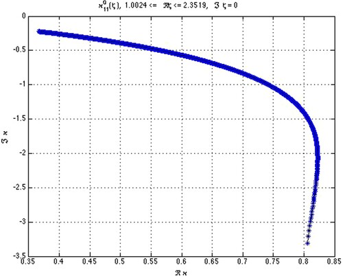
One can independently verify the obtained results. Indeed, representing, in the cylindrical coordinates, the solutions to TEP H for a disk and applying separation of variables [7–9], one arrives at a generalized Fourier (Watson) series where the coefficients have poles at the values of complex spectral parameter that solve the equation (43) $\sqrt{{ϵ}_1}{J}_n^{\prime }(\kappa \sqrt{{ϵ}_1})H_n^{(1)}(\kappa )-J_n(\kappa \sqrt{{ϵ}_1})(H_n^{(1)}{)}^{\prime }(\kappa )=0.$(43) Note that this very equation was considered in [17] in connection with the analysis of fictitious eigenvalues for the dielectric scatterer of circular cross section. The mentioned poles are (a subset of) eigenvalues of TEP H for a disk. Considering the case n = 0 and taking k or κ as a spectral parameter, it can be proved, using the technique [13] and results [12,20] and applying, as in [12], Rouché's theorem, that equation (43(43) $\sqrt{{ϵ}_1}{J}_n^{\prime }(\kappa \sqrt{{ϵ}_1})H_n^{(1)}(\kappa )-J_n(\kappa \sqrt{{ϵ}_1})(H_n^{(1)}{)}^{\prime }(\kappa )=0.$(43) ) has, for every fixed value of the refraction index $\zeta =\sqrt{{ϵ}_1}>0$, exactly one (complex) zero of multiplicity one at a point ${\kappa }_m^{\ast }$ inside ${\mathrm{\Gamma }}_m=\{\kappa :|\kappa -(j_{1,m}/\zeta )|=r_m\}$, $m=1,2,\dots$, of a radius $r_m<d_m/\zeta$ at least beginning from a certain value $m=m_0>1$ of index m. This result perfectly fits formula (42(42) ${\gamma }_{(T,0m)}^{\ast }={\tilde{k}}_{0,m}-g_{(T,0m)},g_{(T,0m)}=\frac{1}{{ϵ}_1+{ϵ}_2}\frac{({\hat{c}}_{0,m}^{-}{)}^2}{\ln 2},m=1,2,\dots ,$(42) ) and the estimates above concerning the location of eigenvalues of TEP H for a disk.

Figure 1 exemplifies the location and evolution of an RF in the fourth quadrant of the complex κ-plane associated with the first (minimal positive) pole of Green's function against the varying refraction index $\zeta$.

Figure 1. Complex zeros ${\kappa }_1^{\ast }(\zeta )$ of (43(43) $\sqrt{{ϵ}_1}{J}_n^{\prime }(\kappa \sqrt{{ϵ}_1})H_n^{(1)}(\kappa )-J_n(\kappa \sqrt{{ϵ}_1})(H_n^{(1)}{)}^{\prime }(\kappa )=0.$(43) ) in the fourth quadrant of the complex κ-plane parametrized by increasing $\mathrm{\Re }\zeta$, $1.0024\le \mathrm{\Re }\zeta \le 2.3519$, $\mathrm{\Im }\zeta =0$, ${\kappa }_1^{\ast }({\zeta }_0)=0.8061-3.3082i$, ${\kappa }_1^{\ast }({\zeta }_S)=0.3661-0.2238i$, and calculated at $\zeta ={\zeta }_0+s{h}_s$, ${\zeta }_0=1.0024$, $s=1,2,\dots ,S=2700$, and $h_s=0.0005$; $1.0048\le ϵ={\zeta }^2\le 5.5314$.

8. Conclusion

We have proved the existence of RFs by reducing the corresponding eigenvalue problems for dielectric cylindrical scatterers of arbitrary cross section to the determination of CNs of Fredholm integral OVFs constructed using Green's potentials. We have verified the occurrence of CNs of the separated OVF principal parts, meromorphic operator pencils, in close proximities of the pencil poles. The obtained pole-pencils CNs are calculated as ‘shifted’ internal eigenvalues using simple formulas and provide good approximations of ‘true’ CNs and the TEP-H eigenvalues. The results have been illustrated and justified by considering a dielectric cylinder of circular cross section.

The single BIE for the determination of the eigenvalue spectrum explored in this work is (a) much simpler than the BIE systems used in many previous studies and (b) provides the possibility of proving the existence, obtaining approximate formulas for eigenvalues, and finding the domain of the RF location.

The results of this work facilitate the understanding of the physical nature of resonance regimes and fictitious resonance modes (eigenvalues) in open dielectric and metal-dielectric resonators. In fact, one may conclude that resonances of a bounded (internal) domain filled with a dielectric medium give rise to RFs of an open structure and cause anomalous scattering in the diffraction problems. Detailed investigations of these issues will be a subject of future studies.

Disclosure statement

No potential conflict of interest was reported by the author(s).

Additional information

Funding

This study is supported by the Russian Science Foundation, project no. 20-11-20087.

Appendix

The table presents the first five zeros $j_{1,m}$ of Bessel function $J_1(z)$, poles ${\tilde{k}}_{0,m}=j_{1,m}$ ($m=1,\dots ,5$), CNs ${\gamma }_{(T,0m)}^{\ast }$, deviations $g_{(T,0m)}$, and differences $j_{1,m+1}-j_{1,m}$ between neighboring zeros of $J_1(z)$ calculated according to (39(39) $\begin{array}{rl}{\hat{c}}_{0,m}^{-}& =-\frac{1}{2\pi }\underset{\tilde{k}\to {\tilde{k}}_{0,m}}{lim}\frac{(\tilde{k}-{\tilde{k}}_{0,m})J_0(\tilde{k}R)}{\tilde{k}R{J}_1(\tilde{k}R)}=-\frac{1}{2\pi }\frac{1}{{\eta }_{0,m}}\frac{J_0({\eta }_{0,m})}{R{J}_1^{\prime }({\eta }_{0,m})}\\ & =\frac{1}{2\pi R}\frac{J_0({\eta }_{0,m})}{{\eta }_{0,m}{J}_2({\eta }_{0,m})-J_1({\eta }_{0,m})},\end{array}$(39) ) and (42(42) ${\gamma }_{(T,0m)}^{\ast }={\tilde{k}}_{0,m}-g_{(T,0m)},g_{(T,0m)}=\frac{1}{{ϵ}_1+{ϵ}_2}\frac{({\hat{c}}_{0,m}^{-}{)}^2}{\ln 2},m=1,2,\dots ,$(42) ) at $R\sqrt{{ϵ}_1}=1$, ${ϵ}_1=4$, and ${ϵ}_2=1$.

Table A1. Zeros $j_{1,m}$ of $J_1(z)$, poles ${\tilde{k}}_{0,m}=j_{1,m}$ ($m=1,\dots ,5$), CNs ${\gamma }_{(T,0m)}^{\ast }$, deviations $g_{(T,0m)}$, and $d_m=j_{1,m+1}-j_{1,m}$, $R\sqrt{{ϵ}_1}=1$, ${ϵ}_1=4$, and ${ϵ}_2=1$.

m	$j_{1,m}$	${\gamma }_{(T,0m)}^{\ast }$	$g_{(T,0m)}$	$j_{1,m+1}-j_{1,m}$
1	3.8317	3.1956	0.6361	3.8317
2	7.0156	7.0136	0.0020	3.1839
3	10.1735	10.1698	0.0037	3.1579
4	13.3237	13.3231	0.0006	3.1502
5	16.4706	16.4698	0.0008	3.1469

References

- Reed M, Simon B. Methods of modern mathemaical physics. New York: Academic; 1978.
- Lax PD, Phillips R. Decaying modes for the wave equation in the exterior of an obstacle. Comm Pure Appl Math. 1969; 22:737–787.
- Agranovich MS, Katsenelenbaum BZ, Sivov AN, et al. Generalized Method of Eigenoscillations in Diffraction Theory. 1st Ed., Weinheim: Wiley-VCH; 1999.
- Shestopalov V, Shestopalov Y. Spectral theory and excitation of open structures. London: IEE Publ; 1995.
- Shestopalov Y, Chernokozhin E. Resonant and nonresonant diffraction by open image-type slotted structures. IEEE Trans Antennas Propag. 2001;49:793–801.
- Hein S, Hohage T, Koch W. On resonances in open systems. J Fluid Mech. 2004;506:255–284.
- van Bladel J. Electromagnetic Fields. Piscataway, NJ: Wiley; 2007. (IEEE Press Series on Electromagnetic Wave Theory). Ch 10.5.
- Wait JR. Scattering of a plane wave from a circular dielectric cylinder at oblique incidence. Canadian J Phys. 1955;33:189–195.
- King RWP, Wu T. The scattering and diffraction of waves. Cambridge, MA: Harvard Univ. Press; 1959.
- Anyutin AP, Korshunov IP, Shatrov AD. High-Q resonances of surface waves in thin metamaterial cylinders. J Commun Technol Electron. 2014;59:1087–1091.
- Shestopalov Y, Okuno Y, Kotik N. Oscillations in slotted resonators with several slots: application of approximate semi-inversion, PIER B, Vol. 39, 2003, pp. 193-247 (Abstract: Journal of Electromagnetic Waves and Applications, Vol. 17, 2003, pp 755-757).
- Shestopalov Y. Complex waves in a dielectric waveguide. Wave Motion. 2018;82:16–19.
- Shestopalov Y. Trigonometric and cylindrical polynomials and their applications in electromagnetics, Applicable analysis, Open access, February 2019.
- Shestopalov Y. On the theory of cylindrical resonators. Math Meths Appl Sci. 1991;14:335–375.
- Shestopalov Y, Smirnov Y, Chernokozhin E. Logarithmic integral equations in electromagnetics. VSP: Utrecht; 2000.
- Spiridonov A, Oktyabrskaya A, Karchevskii E, et al. Mathematical and numerical analysis of the generalized complex-frequency eigenvalue problem for two-dimensional optical microcavities. SIAM J Appl Math. 2020;80:1977–1998.
- Misawa R, Niino K, Nishimura N. Boundary integral equations for calculating complex eigenvalues of transmission problems. SIAM J Appl Math. 2017;77:770–788.
- Poyedinchuk A, Tuchkin Y, Shestopalov V. New Numerical-Analytical methods in diffraction theory. Math Comput Model. 2000;32:1029–1046.
- Koshparenok V, Melezhik P, Poyedinchuk A, et al. Spectral theory of open two-dimensional resonators with dielectric inclusions. USSR Comp Maths Math Phys. 1985;25:151–161.
- Shestopalov Y. Resonant states in waveguide transmission problems. Prog Electromagnetics Res B. 2015;64:119–143.
- Gohberg I. Operator theory and boundary eigenvalue problems. Basel: Birkhäuser; 1995.
- Gohberg I, Leiterer J. Holomorphic operator functions of one variable and applications. Basel: Birkhäuser; 2009. (Operator Theory: Advances and Applications; vol. 192).
- Shestopalov Y. Justification of a method for calculating the normal waves. Vestnik Mosk Gos Univ Ser. 1979;15(1):14–20.
- Shestopalov Y. Justification of the spectral method for calculating normal waves of transmission lines. Diff Uravn. 1980;16:1504–1512.
- Shestopalov Y. On the spectrum of a family of non-self-adjoint boundary value problems for systems of helmholtz equations. USSR Com Math Math Phys. 1981;21:97–108.
- Poyedinchuk A. Discrete spectrum of one class of open cylindrical structures. Dopov Ukrain Akad Nauk. 1983;48–52.
- Il'inskii AS, Shestopalov Y. Applications of the methods of spectral theory in the problems of wave propagation. Moscow: Moscow University Press; 1989.
- Chernokozhin E, Shestopalov Y. A method of calculating the characteristic numbers of a meromorphic operator-function. USSR Com Math Math Phys. 1985;25:89–91.
- Shestopalov Y. Normal modes of bare and shielded slot lines formed by domains of arbitrary cross section. Dokl Akad Nauk SSSR. 1986;289:616–618.
- Shestopalov Y. Application of the method of generalized potentials to the solution of certain problems in the theory of the diffraction and propagation of waves. USSR Com Math Math Phys. 1990;30:83–91.
- Shestopalov Y. Potential theory for the Helmholtz operator and nonlinear eigenvalue problems. In: M. Kishi, editors. Potential Theory. Berlin, New York: W. de Gruyter; 1992. pp. 281–290.
- Shestopalov Y. Non-linear eigenvalue problems in electrodynamics. Electromagnetics. 1993;13:133–143.
- Shestopalov Y. Calculation of open slotted structures with layered dielectric filling. Proceedings SPIE 2211; 1994. (Millimeter and Submillimeter Waves).
- Shestopalov Y. Scattering frequencies in planar domains with noncompact boundaries. In: E. Meister, editors. Modern mathematical methods in diffraction theory and its applications in engineering. Frankfurt am Main: Peter Lang; 1997. p. 227–233.
- Shestopalov Y, Chernokozhin E. Solvability of boundary value problems for the helmholtz equation in an unbounded domain with noncompact boundary. Diff Equ. 1998;34:546–553.
- Shestopalov Y, Smirnov Y. The diffraction in a class of unbounded domains connected through a hole. Math Meths Appl Sci. 2003;26:1363–1389.
- Ammari H, Kang H, Lim M, Zribi H. Layer potential techniques in spectral analysis. Part I: complete asymptotic expansions for eigenvalues of the Laplacian in domains with small inclusions. Trans Am Math Soc. 2010;362:2901–2922.
- Ammari H, Kang H, Lee H. Layer potential techniques in spectral analysis. Providence, RI: AMS; 2009. (Mathematical Surveys and Monographs; vol. 153).
- Il'inskii AS, Chernokozhin EV. Inversion of a logarithmic operator defined on a regular set of arcs lying on a circle. Comp Math Math Phys. 2009;49:1415–1428.
- Roach GF. Green's functions: introductory theory with applications. London: Van Nostrand Reinhold; 1970.
- Cakoni F, Haddar H. Transmission eigenvalues in inverse scattering theory, Gunther Uhlmann. Inside Out II, 60, MSRI Publications, p. 527–578, 2012.
- Colton D, Kress RIntegral equation methods in scattering theory. NY: Wiley; 1983.
- Krutitskii PA. The neumann problem for the 2-d Helmholtz equation in a domain, bounded by closed and open curves. Int J Math Math Sci. 1998;21:209–216.
- Gabdulkhaev B. Direct methods of solution to singular integral equations of the first kind. Kazan: Kazan State University; 1994.
- Gakhov F. Boundary value problems. Oxford: Pergamon; 1966.
- Samko S. Hypersingular integrals and their applications. Boca Raton, FL: CRC Press; 2014.
- Gesztesy F, Holden H, Nicholls R. On factorizations of analytic operator-valued functions and eigenvalue multiplicity questions. Integral Eqs Operator Theory. 2015;82:61–94.
- Gohberg I, Sigal EN. The operator generalization of a theorem on logarithmic residue and the Rouché theorem. Mat Sb. 1971;84:607–629.
- Steinberg S. Meromorphic families of compact operators. Arch Rational Mech Anal. 1968;31:372–379.
- Sanchez-Palencia E. Inhomogeneous media and vibration theory. NY: Springer; 1980. (Lecture Notes in Physics; vol. 127).
Appendix
The table presents the first five zeros of Bessel function
, poles
(
), CNs
, deviations
, and differences
between neighboring zeros of
calculated according to (Equation39
(39)
(39) ) and (Equation42
(42)
(42) ) at
,
, and
.
Table A1. Zeros of