Exact solutions for geophysical flows with discontinuous variable density and forcing terms in spherical coordinates

ABSTRACT

We present here exact solutions to the equations of geophysical fluid dynamics that depict inviscid flows moving in the azimuthal direction on a circular path, around the globe, and which admit a velocity profile below the surface and along it. These features render this model suitable for the description of the Antarctic circumpolar current (ACC). The governing equations we work with–taken to be the Euler equations written in spherical coordinates–also incorporate forcing terms which are generally regarded as means that ensure the general balance of the ACC. Our approach allows for a variable density (depending on the depth and latitude) of discontinuous type which divides the water domain into two layers. Thus, the discontinuity gives rise to an interface. The velocity in both layers and the pressure in the lower layer are determined explicitly, while the pressure in the upper layer depends on the free surface and the interface. Functional analytical techniques render (uniquely) the surface and interface-defining functions in an implicit way. We conclude our discussion by deriving relations between the monotonicity of the surface pressure and the monotonicity of the surface distortion that concur with the physical expectations. A regularity result concerning the interface is also derived.

KEYWORDS:

• Exact solutions in spherical coordinates
• discontinuous stratification
• Coriolis force
• forcing terms
• the Antarctic Circumpolar Current

MATHEMATICS SUBJECT CLASSIFICATIONS:

• Primary: 35Q31
• 35Q35
• Secondary: 35Q86

1. Introduction

We present here a mathematical perspective concerning geophysical water flows exhibiting stratification, internal waves and a preferred (azimuthal) propagation direction. This task is carried out by deriving and analysing a family of exact solutions to the geophysical water wave equations written in spherical coordinates, in a rotating coordinate frame with the origin at a point on the Earth's surface that moves with the Earth and which incorporates forcing terms. These solutions describe incompressible, inviscid, stratified, steady flows moving on a circular path in the azimuthal direction completely around the globe and possessing a velocity profile below the surface and along it.

The previously mentioned aspects greatly apply to the Antarctic circumpolar current (Antarctic circumpolar current)—the only major current that circumnavigates the globe flowing eastwards through the southern regions of the Atlantic, Indian and Pacific Oceans along 23,000 km and having (in places) a width of over 2000 km, cf. Refs. [1–4]. More precisely, the earlier mentioned forcing terms provide the dynamical balance of ACC, cf. Refs. [5,6].

An important feature of geophysical flows, also discussed here, is stratification. Indeed, it is known [7,8] that in the southern oceans, strong meridional changes in air-sea buoyancy flux give rise to a strong polar front along which the ACC flows in thermal wind balance with the density gradients. One way in which stratification emerges is through eddies: it is argued in Ref. [7] that in collusion with imposed patterns of mechanical and buoyancy forcing, the eddies can set the stratification in both horizontal and vertical directions. Stratification also accommodates observed sharp changes in water density (due to variations in temperature and salinity, cf. Refs. [9–13]), known as fronts or jets, cf. Ref. [14].

In regard to the aspects mentioned earlier, we consider here a discontinuous density stratification of general type: mindful of the earlier described stratification induced by eddies, we allow the density to vary in the horizontal and vertical directions. Thus, in terms of spherical coordinates, the density that we consider here varies in the radial and latitudinal coordinates, respectively.

Although complicated analytical issues concerning stratification were dealt with in the case of two-dimensional flows, cf. Refs. [9,15–27], progress on the important issue of stratification in geophysical flows materialized only relatively recently, after the important developments by Constantin and Johnson [5,28] who constructed by means of spherical coordinates exact solutions to the geophysical fluid dynamics (GFD) equations representing azimuthal, depth-varying flows of constant density, which were able to capture the salient features of the equatorial undercurrent (EUC) and ACC, respectively. For a selective list of recent works concerning exact solutions in GFD, we refer to Refs. [5,9,10,28–40]. Building upon the approaches in Refs. [5,28], Henry and Martin [41–43] constructed exact solutions to GFD representing equatorial flows with continuously varying density depending on depth and latitude. This type of approach was extended to include discontinuous density, cf. Ref. [38], and discontinuously varying density together with forcing terms, cf. Refs. [44,45]. Here, we extend previous approaches [5,44,46–49] (regarding exact solutions pertaining to EUC and ACC) and so include forcing terms in the presence of a density stratification that varies (discontinuously) with respect to depth and latitude: we allow a vertical layering of the flow, with two layers of different, non-constant densities, where the denser layer sits below the less dense one (stable stratification). The discontinuity in density gives rise to an interface that behaves like an internal wave [7,8,18–20,50,51].

The layout of the paper is as follows: we introduce in Section 2 the governing equations (in spherical coordinates) and their boundary conditions for geophysical flows. Thereafter, we derive in Section 3 explicit solutions for the velocity field and the corresponding pressure function in the two layers of the fluid domain. From the dynamic boundary condition, we find an implicit relation between the imposed pressure and the resulting surface distortion. The interface defining function appears also implicitly as a condition expressing the balance of forces at the interface. In conjunction with the implicit function theorem, the two implicit equations are used to prove that any small enough perturbation of the pressure required to preserve an undisturbed free surface (following the curvature of the Earth) triggers unique functions, describing the surface and the interface, respectively. Finally, we prove that the solution we derived displays expected physical properties: a decay of the surface height occurs as soon as the pressure along the free surface increases. Moreover, we also prove that the interface defining function has very good regularity properties.

2. Physical problem and governing equations

In this section, we provide the governing equations for geophysical flows written in spherical coordinates to accommodate the shape of the Earth, together with the boundary conditions for the free surface and a rigid bed.

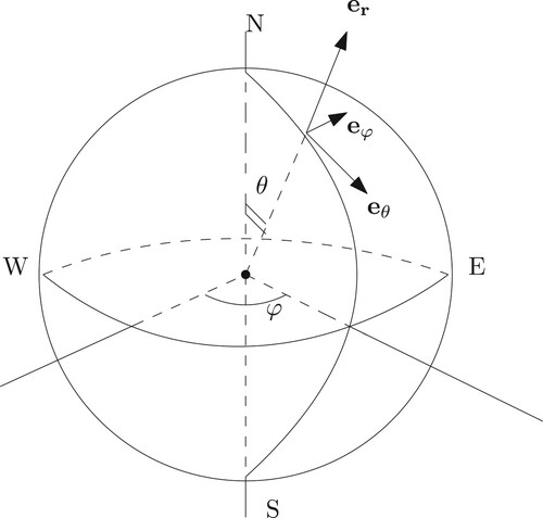
We will work in a system of right handed coordinates $(r,\theta ,\phi )$ where r denotes the distance to the centre of the sphere, $\theta \in [0,\pi ]$ is the polar angle (the convention being that $\pi /2-\theta$ is the angle of latitude) and $\phi \in [0,2\pi ]$ is the azimuthal angle (the angle of longitude). While in this coordinate system the North and South poles are located at $\theta =0,\pi$, respectively, the Equator sits on $\theta =\pi /2$, and the ACC is situated at $\theta =3\pi /4$. The unit vectors in this system are $\begin{array}{rl}{\mathbf{e}}_r& =(\sin \mathrm{\theta cos}\phi ,\sin \mathrm{\theta sin}\phi ,\cos \theta ),\\ {\mathbf{e}}_{\theta }& =(\cos \mathrm{\theta cos}\phi ,\cos \mathrm{\theta sin}\phi ,-\sin \theta ),\\ {\mathbf{e}}_{\phi }& =(-\sin \phi ,\cos \phi ,0)\end{array}$with ${\mathbf{e}}_{\phi }$ pointing from West to East and ${\mathbf{e}}_{\theta }$ from North to South, cf. Figure 1.

Figure 1. The spherical coordinate system: θ is the polar angle, φ is the azimuthal angle (the angle of longitude) and r represents the distance to the origin.

Throughout this paper, we make the following simplifying assumption on the location of the ACC. We assume that the angle of latitude θ lies in the compact interval $I_{\theta }$: (1) $\theta \in I_{\theta }:=[\frac{3\pi }{4}-\frac{\pi }{18},\frac{3\pi }{4}+\frac{\pi }{18}].$(1) We are guided in our study by the observations made in Ref. [52] asserting that the Reynolds number is, in general, extremely large for oceanic flows. Accordingly, we will consider incompressible and inviscid flows. For $0<r_2<r_1\ll R$ and $R_j:=R+r_j$, j = 1, 2, we consider the two fluid layers $D_j$ separated by an interface and bounded by the bottom and a free surface, which are described by the graphs of the functions h, d and k, respectively: $\begin{array}{rl}{D}_1& :=\left\{\right(r,\theta ,\phi ):R_2+h(\theta ,\phi )\le r\le R_1+k(\theta ,\phi \left)\right\},\\ D_2& :=\left\{\right(r,\theta ,\phi ):R+d(\theta ,\phi )\le r\le R_2+h(\theta ,\phi \left)\right\}.\end{array}$We associate R with the Earth's radius. The given function d describes the bottom topography, whereas h and k describe the unknown deviations of the interface and the free surface from their unperturbed locations at $R_2$ and $R_1$, respectively. In particular, the density, ρ, is discontinuous with a jump at the interface $R_2+h$. More precisely, $\rho ={\rho }_1(r,\theta )$ in $D_1$ and $\rho ={\rho }_2(r,\theta )$ in $D_2$.

Let $\mathbf{u}=w{\mathbf{e}}_r+v{\mathbf{e}}_{\theta }+u{\mathbf{e}}_{\phi }.$Then the Euler equations in the rotating frame for $(w_j,v_j,u_j)$ within $D_j$, j = 1, 2, are given by (2) $\begin{array}{rl}& w_{j,t}+w_j{w}_{j,r}+\frac{v_j}{r}{w}_{j,\theta }+\frac{u_j}{\mathrm{rsin}\theta }{w}_{j,\phi }-\frac{1}{r}(v_j^2+u_j^2)-2\mathrm{\Omega }{u}_j\sin \theta -r{\mathrm{\Omega }}^2{\sin }^2\theta \\ & =-\frac{p_{j,r}}{\rho }+{\mathfrak{F}}_j^r,\\ & v_{j,t}+w_j{v}_{j,r}+\frac{v_j}{r}{v}_{j,\theta }+\frac{u_j}{\mathrm{rsin}\theta }{v}_{j,\phi }+\frac{1}{r}(w_j{v}_j-u_j^2\cot \theta )-2\mathrm{\Omega }{u}_j\cos \theta -r{\mathrm{\Omega }}^2\sin \mathrm{\theta cos}\theta \\ & =-\frac{p_{j,\theta }}{\mathrm{r\rho }}+{\mathfrak{F}}_j^{\theta },\\ & u_{j,t}+w_j{u}_{j,r}+\frac{v_j}{r}{u}_{j,\theta }+\frac{u_j}{\mathrm{rsin}\theta }{u}_{j,\phi }+\frac{1}{r}(w_j{u}_j+v_j{u}_j\cot \theta )+2\mathrm{\Omega }{w}_j\sin \theta +2\mathrm{\Omega }{v}_j\cos \theta \\ & =-\frac{p_{j,\phi }}{\mathrm{r\rho sin}\theta }+{\mathfrak{F}}_j^{\phi },\end{array}$(2) which incorporate both Coriolis effects and centripetal acceleration ($\mathrm{\Omega }\approx 7.29\times {10}^{-5}\mathrm{rad}{\mathrm{s}}^{-1}$ refers to the constant rotation speed of the Earth), cf. Ref. [28]. Here, $p_j(r,\theta ,\phi )$ denotes the pressure field and ${\mathfrak{F}}_j=({\mathfrak{F}}_j^r{\mathbf{e}}_r,{\mathfrak{F}}_j^{\theta }{\mathbf{e}}_{\theta },{\mathfrak{F}}_j^{\phi }{\mathbf{e}}_{\phi })$ is the body-force vector. Additionally to (2(2) $\begin{array}{rl}& w_{j,t}+w_j{w}_{j,r}+\frac{v_j}{r}{w}_{j,\theta }+\frac{u_j}{\mathrm{rsin}\theta }{w}_{j,\phi }-\frac{1}{r}(v_j^2+u_j^2)-2\mathrm{\Omega }{u}_j\sin \theta -r{\mathrm{\Omega }}^2{\sin }^2\theta \\ & =-\frac{p_{j,r}}{\rho }+{\mathfrak{F}}_j^r,\\ & v_{j,t}+w_j{v}_{j,r}+\frac{v_j}{r}{v}_{j,\theta }+\frac{u_j}{\mathrm{rsin}\theta }{v}_{j,\phi }+\frac{1}{r}(w_j{v}_j-u_j^2\cot \theta )-2\mathrm{\Omega }{u}_j\cos \theta -r{\mathrm{\Omega }}^2\sin \mathrm{\theta cos}\theta \\ & =-\frac{p_{j,\theta }}{\mathrm{r\rho }}+{\mathfrak{F}}_j^{\theta },\\ & u_{j,t}+w_j{u}_{j,r}+\frac{v_j}{r}{u}_{j,\theta }+\frac{u_j}{\mathrm{rsin}\theta }{u}_{j,\phi }+\frac{1}{r}(w_j{u}_j+v_j{u}_j\cot \theta )+2\mathrm{\Omega }{w}_j\sin \theta +2\mathrm{\Omega }{v}_j\cos \theta \\ & =-\frac{p_{j,\phi }}{\mathrm{r\rho sin}\theta }+{\mathfrak{F}}_j^{\phi },\end{array}$(2) ), the equation of mass conservation is required to be satisfied: (3) $\frac{1}{r^2}\frac{\mathrm{\partial }}{\mathrm{\partial }r}\left(r^2\rho w_j\right)+\frac{1}{\mathrm{rsin}\theta }\frac{\mathrm{\partial }}{\mathrm{\partial }\theta }(\rho v_j\sin \theta )+\frac{1}{\mathrm{rsin}\theta }\frac{\mathrm{\partial }}{\mathrm{\partial }\phi }\left(\rho u_j\right)=0.$(3) The GFD (2(2) $\begin{array}{rl}& w_{j,t}+w_j{w}_{j,r}+\frac{v_j}{r}{w}_{j,\theta }+\frac{u_j}{\mathrm{rsin}\theta }{w}_{j,\phi }-\frac{1}{r}(v_j^2+u_j^2)-2\mathrm{\Omega }{u}_j\sin \theta -r{\mathrm{\Omega }}^2{\sin }^2\theta \\ & =-\frac{p_{j,r}}{\rho }+{\mathfrak{F}}_j^r,\\ & v_{j,t}+w_j{v}_{j,r}+\frac{v_j}{r}{v}_{j,\theta }+\frac{u_j}{\mathrm{rsin}\theta }{v}_{j,\phi }+\frac{1}{r}(w_j{v}_j-u_j^2\cot \theta )-2\mathrm{\Omega }{u}_j\cos \theta -r{\mathrm{\Omega }}^2\sin \mathrm{\theta cos}\theta \\ & =-\frac{p_{j,\theta }}{\mathrm{r\rho }}+{\mathfrak{F}}_j^{\theta },\\ & u_{j,t}+w_j{u}_{j,r}+\frac{v_j}{r}{u}_{j,\theta }+\frac{u_j}{\mathrm{rsin}\theta }{u}_{j,\phi }+\frac{1}{r}(w_j{u}_j+v_j{u}_j\cot \theta )+2\mathrm{\Omega }{w}_j\sin \theta +2\mathrm{\Omega }{v}_j\cos \theta \\ & =-\frac{p_{j,\phi }}{\mathrm{r\rho sin}\theta }+{\mathfrak{F}}_j^{\phi },\end{array}$(2) ) and (3(3) $\frac{1}{r^2}\frac{\mathrm{\partial }}{\mathrm{\partial }r}\left(r^2\rho w_j\right)+\frac{1}{\mathrm{rsin}\theta }\frac{\mathrm{\partial }}{\mathrm{\partial }\theta }(\rho v_j\sin \theta )+\frac{1}{\mathrm{rsin}\theta }\frac{\mathrm{\partial }}{\mathrm{\partial }\phi }\left(\rho u_j\right)=0.$(3) ) are supplemented with the following boundary conditions. At the free surface $r=R_1+k(\theta ,\phi )$, we require the dynamic boundary condition (4) $p_1=P_1(\theta ,\phi )$(4) (for a prescribed function $P_1$) and the kinematic boundary condition (5) $w_1=\frac{v_1}{r}\frac{\mathrm{\partial }k}{\mathrm{\partial }\theta }+\frac{u_1}{\mathrm{rsin}\theta }\frac{\mathrm{\partial }k}{\mathrm{\partial }\phi }$(5) to be satisfied. At the interface $r=R_2+h(\theta ,\phi )$, we require the normal components of the velocity fields ${\mathbf{u}}_j$ to be equal: (6) $\begin{array}{rl}& (w_1{\mathbf{e}}_r+v_1{\mathbf{e}}_{\theta }+u_1{\mathbf{e}}_{\phi })\cdot ({\mathbf{e}}_r-\frac{h_{\theta }}{r}{\mathbf{e}}_{\theta }-\frac{h_{\phi }}{\mathrm{rsin}\theta }{\mathbf{e}}_{\phi })\\ & =(w_2{\mathbf{e}}_r+v_2{\mathbf{e}}_{\theta }+u_2{\mathbf{e}}_{\phi })\cdot ({\mathbf{e}}_r-\frac{h_{\theta }}{r}{\mathbf{e}}_{\theta }-\frac{h_{\phi }}{\mathrm{rsin}\theta }{\mathbf{e}}_{\phi }).\end{array}$(6) Moreover, to ensure the balance of forces, we require that (7) $p_1=p_2\mathrm{on}{R}_2+h(\theta ,\phi ).$(7) At the rigid ocean bottom $r=d(\theta ,\phi )$, it holds that (8) $w_2=\frac{v_2}{r}\frac{\mathrm{\partial }d}{\mathrm{\partial }\theta }+\frac{u_2}{\mathrm{rsin}\theta }\frac{\mathrm{\partial }d}{\mathrm{\partial }\phi }.$(8)

3. Exact solutions

This section is concerned with the derivation of exact solutions to the problem (2(2) $\begin{array}{rl}& w_{j,t}+w_j{w}_{j,r}+\frac{v_j}{r}{w}_{j,\theta }+\frac{u_j}{\mathrm{rsin}\theta }{w}_{j,\phi }-\frac{1}{r}(v_j^2+u_j^2)-2\mathrm{\Omega }{u}_j\sin \theta -r{\mathrm{\Omega }}^2{\sin }^2\theta \\ & =-\frac{p_{j,r}}{\rho }+{\mathfrak{F}}_j^r,\\ & v_{j,t}+w_j{v}_{j,r}+\frac{v_j}{r}{v}_{j,\theta }+\frac{u_j}{\mathrm{rsin}\theta }{v}_{j,\phi }+\frac{1}{r}(w_j{v}_j-u_j^2\cot \theta )-2\mathrm{\Omega }{u}_j\cos \theta -r{\mathrm{\Omega }}^2\sin \mathrm{\theta cos}\theta \\ & =-\frac{p_{j,\theta }}{\mathrm{r\rho }}+{\mathfrak{F}}_j^{\theta },\\ & u_{j,t}+w_j{u}_{j,r}+\frac{v_j}{r}{u}_{j,\theta }+\frac{u_j}{\mathrm{rsin}\theta }{u}_{j,\phi }+\frac{1}{r}(w_j{u}_j+v_j{u}_j\cot \theta )+2\mathrm{\Omega }{w}_j\sin \theta +2\mathrm{\Omega }{v}_j\cos \theta \\ & =-\frac{p_{j,\phi }}{\mathrm{r\rho sin}\theta }+{\mathfrak{F}}_j^{\phi },\end{array}$(2) )–(8(8) $w_2=\frac{v_2}{r}\frac{\mathrm{\partial }d}{\mathrm{\partial }\theta }+\frac{u_2}{\mathrm{rsin}\theta }\frac{\mathrm{\partial }d}{\mathrm{\partial }\phi }.$(8) ). We first establish explicit formulas for the velocity field and the pressure in the layers $D_1$ and $D_2$. Subsequently, we prove an existence type result for the surface and interface defining functions, respectively, by exploiting the balance of forces at the interface between the two fluid domains $D_1$ and $D_2$.

3.1. The velocity field and the pressure

We seek a steady flow governed by (2(2) $\begin{array}{rl}& w_{j,t}+w_j{w}_{j,r}+\frac{v_j}{r}{w}_{j,\theta }+\frac{u_j}{\mathrm{rsin}\theta }{w}_{j,\phi }-\frac{1}{r}(v_j^2+u_j^2)-2\mathrm{\Omega }{u}_j\sin \theta -r{\mathrm{\Omega }}^2{\sin }^2\theta \\ & =-\frac{p_{j,r}}{\rho }+{\mathfrak{F}}_j^r,\\ & v_{j,t}+w_j{v}_{j,r}+\frac{v_j}{r}{v}_{j,\theta }+\frac{u_j}{\mathrm{rsin}\theta }{v}_{j,\phi }+\frac{1}{r}(w_j{v}_j-u_j^2\cot \theta )-2\mathrm{\Omega }{u}_j\cos \theta -r{\mathrm{\Omega }}^2\sin \mathrm{\theta cos}\theta \\ & =-\frac{p_{j,\theta }}{\mathrm{r\rho }}+{\mathfrak{F}}_j^{\theta },\\ & u_{j,t}+w_j{u}_{j,r}+\frac{v_j}{r}{u}_{j,\theta }+\frac{u_j}{\mathrm{rsin}\theta }{u}_{j,\phi }+\frac{1}{r}(w_j{u}_j+v_j{u}_j\cot \theta )+2\mathrm{\Omega }{w}_j\sin \theta +2\mathrm{\Omega }{v}_j\cos \theta \\ & =-\frac{p_{j,\phi }}{\mathrm{r\rho sin}\theta }+{\mathfrak{F}}_j^{\phi },\end{array}$(2) ) with ${\mathfrak{F}}_j(r,\theta ):=(-g,G(r,\theta ),0)$, where g is the gravity of Earth and G denotes a general body force vector in θ direction, and (3(3) $\frac{1}{r^2}\frac{\mathrm{\partial }}{\mathrm{\partial }r}\left(r^2\rho w_j\right)+\frac{1}{\mathrm{rsin}\theta }\frac{\mathrm{\partial }}{\mathrm{\partial }\theta }(\rho v_j\sin \theta )+\frac{1}{\mathrm{rsin}\theta }\frac{\mathrm{\partial }}{\mathrm{\partial }\phi }\left(\rho u_j\right)=0.$(3) ) together with (4(4) $p_1=P_1(\theta ,\phi )$(4) )–(8(8) $w_2=\frac{v_2}{r}\frac{\mathrm{\partial }d}{\mathrm{\partial }\theta }+\frac{u_2}{\mathrm{rsin}\theta }\frac{\mathrm{\partial }d}{\mathrm{\partial }\phi }.$(8) ), which propagates purely in the azimuthal direction and does not depend on φ. Therefore, the velocity field satisfies $w_j=v_j=0$ and $u_j=u_j(r,\theta )$, $p_j=p_j(r,\theta )$, $h=h\left(\theta \right)$, $k=k\left(\theta \right)$, and for consistency $d=d\left(\theta \right)$. Without loss of generality, we will assume that (9) $h\left(\frac{3\pi }{4}\right)=0.$(9) Then (3(3) $\frac{1}{r^2}\frac{\mathrm{\partial }}{\mathrm{\partial }r}\left(r^2\rho w_j\right)+\frac{1}{\mathrm{rsin}\theta }\frac{\mathrm{\partial }}{\mathrm{\partial }\theta }(\rho v_j\sin \theta )+\frac{1}{\mathrm{rsin}\theta }\frac{\mathrm{\partial }}{\mathrm{\partial }\phi }\left(\rho u_j\right)=0.$(3) ) and (4(4) $p_1=P_1(\theta ,\phi )$(4) )–(8(8) $w_2=\frac{v_2}{r}\frac{\mathrm{\partial }d}{\mathrm{\partial }\theta }+\frac{u_2}{\mathrm{rsin}\theta }\frac{\mathrm{\partial }d}{\mathrm{\partial }\phi }.$(8) ) are automatically satisfied, while the Euler equations reduce to (10) $\{\begin{array}{c}-\frac{u_j^2}{r}-2\mathrm{\Omega }{u}_j\sin \theta -r{\mathrm{\Omega }}^2{\sin }^2\theta =-\frac{p_{j,r}}{\rho }-g,\\ -\frac{u_j^2}{r}\cot \theta -2\mathrm{\Omega }{u}_j\cos \theta -r{\mathrm{\Omega }}^2\sin \mathrm{\theta cos}\theta =-\frac{p_{j,\theta }}{\mathrm{\rho r}}+G(r,\theta ),\\ 0=p_{j,\phi }.\end{array}$(10)

Remark 3.1

Concerning the nature of the forcing term above, it is argued in Ref. [5] that a relevant choice is (11) $G(r,\theta )=-2\mathrm{\Omega }{u}_0\cos \theta ,$(11) where $u_0$ is the velocity of a linear flow which comes about by ignoring the nonlinear advection terms in (10(10) $\{\begin{array}{c}-\frac{u_j^2}{r}-2\mathrm{\Omega }{u}_j\sin \theta -r{\mathrm{\Omega }}^2{\sin }^2\theta =-\frac{p_{j,r}}{\rho }-g,\\ -\frac{u_j^2}{r}\cot \theta -2\mathrm{\Omega }{u}_j\cos \theta -r{\mathrm{\Omega }}^2\sin \mathrm{\theta cos}\theta =-\frac{p_{j,\theta }}{\mathrm{\rho r}}+G(r,\theta ),\\ 0=p_{j,\phi }.\end{array}$(10) ).

We remark that the system (10(10) $\{\begin{array}{c}-\frac{u_j^2}{r}-2\mathrm{\Omega }{u}_j\sin \theta -r{\mathrm{\Omega }}^2{\sin }^2\theta =-\frac{p_{j,r}}{\rho }-g,\\ -\frac{u_j^2}{r}\cot \theta -2\mathrm{\Omega }{u}_j\cos \theta -r{\mathrm{\Omega }}^2\sin \mathrm{\theta cos}\theta =-\frac{p_{j,\theta }}{\mathrm{\rho r}}+G(r,\theta ),\\ 0=p_{j,\phi }.\end{array}$(10) ) can be written as (12) $\begin{array}{r}\{\begin{array}{c}\rho \frac{(u_j+\mathrm{\Omega }\mathrm{rsin}\theta {)}^2}{r}=p_{j,r}+\mathrm{g\rho },\\ \rho (u_j+\mathrm{\Omega rsin}\theta {)}^2\cot \theta =p_{j,\theta }-\mathrm{\rho rG}(r,\theta ).\end{array}\end{array}$(12) The shape of the previous system calls for the elimination of the pressure. Indeed, denoting ${\mathcal{U}}_j(r,\theta ):=\frac{(u_j+\mathrm{\Omega }\mathrm{rsin}\theta {)}^2}{r}$for j = 1, 2, we obtain that ${\mathcal{U}}_j$ satisfies (13) $\sin \theta \frac{\mathrm{\partial }\left(\rho \right(r,\theta \left)r{\mathcal{U}}_j\right)}{\mathrm{\partial }\theta }-\mathrm{rcos}\theta \frac{\mathrm{\partial }\left(\rho \right(r,\theta \left)r{\mathcal{U}}_j\right)}{\mathrm{\partial }r}=\mathrm{rsin}\theta (g{\rho }_{\theta }+\frac{\mathrm{\partial }\left(\mathrm{\rho rG}\right)}{\mathrm{\partial }r})$(13) in $D_j$, j = 1, 2. Utilizing the method of characteristics (cf. Ref. [42]), we infer from the previous equation that the azimuthal velocity $u_j(j=1,2)$ is given as (14) $\begin{array}{rl}{u}_j(r,\theta )& =-\mathrm{\Omega rsin}\theta \\ & +\sqrt{\frac{F_j(\mathrm{rsin}\theta )+\mathrm{rsin}\theta {\int }_0^{f\left(\theta \right)}\left[H_{j,r}\right(\overline{r}\left(s\right),\overline{\theta }\left(s\right))+g{\rho }_{j,\theta }(\overline{r}\left(s\right),\overline{\theta }\left(s\right)\left)\right]\mathrm{d}s}{{\rho }_j(r,\theta )}}\end{array}$(14) for some arbitrary continuously differentiable functions $x\mapsto F_j\left(x\right)$, j = 1, 2, differentiable functions and (15) $\begin{array}{rl}f\left(\theta \right)& :=\frac{1}{2}\ln \frac{1-\cos \theta }{1+\cos \theta },H_j(r,\theta ):=r{\rho }_j(r,\theta )G(r,\theta ){|}_{r\in D_j},\\ \overline{r}\left(s\right)& :=\mathrm{rsin}\mathrm{\theta cosh}\left(s\right),\overline{\theta }\left(s\right):=\arccos (-\sinh (s\left)\right).\end{array}$(15) Plugging (14(14) $\begin{array}{rl}{u}_j(r,\theta )& =-\mathrm{\Omega rsin}\theta \\ & +\sqrt{\frac{F_j(\mathrm{rsin}\theta )+\mathrm{rsin}\theta {\int }_0^{f\left(\theta \right)}\left[H_{j,r}\right(\overline{r}\left(s\right),\overline{\theta }\left(s\right))+g{\rho }_{j,\theta }(\overline{r}\left(s\right),\overline{\theta }\left(s\right)\left)\right]\mathrm{d}s}{{\rho }_j(r,\theta )}}\end{array}$(14) ) into (12(12) $\begin{array}{r}\{\begin{array}{c}\rho \frac{(u_j+\mathrm{\Omega }\mathrm{rsin}\theta {)}^2}{r}=p_{j,r}+\mathrm{g\rho },\\ \rho (u_j+\mathrm{\Omega rsin}\theta {)}^2\cot \theta =p_{j,\theta }-\mathrm{\rho rG}(r,\theta ).\end{array}\end{array}$(12) ) yields that (16a) $\begin{array}{rl}{p}_{j,r}& =-g{\rho }_j(r,\theta )+\frac{F_j(\mathrm{rsin}\theta )}{r}+\sin \theta {\int }_0^{f\left(\theta \right)}\left[H_{j,r}\right(\overline{r}\left(s\right),\overline{\theta }\left(s\right))+g{\rho }_{j,\theta }(\overline{r}\left(s\right),\overline{\theta }\left(s\right)\left)\right]\mathrm{d}s,\end{array}$(16a) (16b) $\begin{array}{rl}{p}_{j,\theta }& =H_j(r,\theta )+\cot \theta \left(F_j\right(\mathrm{rsin}\theta )+\mathrm{rsin}\theta {\int }_0^{f\left(\theta \right)}\left[H_{j,r}\right(\overline{r}\left(s\right),\overline{\theta }\left(s\right))+g{\rho }_{j,\theta }(\overline{r}\left(s\right),\overline{\theta }\left(s\right)\left)\right]\mathrm{d}s).\end{array}$(16b) Introducing the change of variables $y=\mathrm{rsin}\theta$ and integrating (16a(16a) $\begin{array}{rl}{p}_{j,r}& =-g{\rho }_j(r,\theta )+\frac{F_j(\mathrm{rsin}\theta )}{r}+\sin \theta {\int }_0^{f\left(\theta \right)}\left[H_{j,r}\right(\overline{r}\left(s\right),\overline{\theta }\left(s\right))+g{\rho }_{j,\theta }(\overline{r}\left(s\right),\overline{\theta }\left(s\right)\left)\right]\mathrm{d}s,\end{array}$(16a) ) for $r\in [R+d(\theta ),R_2+h(\theta \left)\right]$ leads to (17) $p_2(r,\theta )=-g{\int }_{R+d\left(\theta \right)}^r{\rho }_2(r^{\prime },\theta )\mathrm{d}{r}^{\prime }+{\int }_{(R+d(\theta \left)\right)\sin \theta }^{\mathrm{rsin}\theta }[\frac{F_2\left(y\right)}{y}+{\mathcal{F}}_2(y,\theta \left)\right]\mathrm{d}y+C_2\left(\theta \right),$(17) where $\theta \to C_2\left(\theta \right)$ is a function such that (18) $\begin{array}{rl}{C}_2^{\prime }\left(\theta \right)& =H_2(R+d(\theta ),\theta )-g{\rho }_2(R+d(\theta ),\theta )d^{\prime }\left(\theta \right)\\ & +[\frac{F_2\left(\right(R+d\left(\theta \right))\sin \theta )}{(R+d(\theta \left)\right)\sin \theta }+{\mathcal{F}}_2((R+d(\theta \left)\right)\sin \left(\theta \right),\theta \left)\right]\left(\right(R+d\left(\theta \right))\sin (\theta ){)}^{\prime }\end{array}$(18) and ${\mathcal{F}}_j(y,\theta ):={\int }_0^{f\left(\theta \right)}[H_{j,r}(\mathrm{ycosh}(s),\overline{\theta }(s\left)\right)+g{\rho }_{j,\theta }(\mathrm{ycosh}(s),\overline{\theta }(s\left)\right)]\mathrm{d}s\text{for}j=1,2.$Denoting ${\mathcal{F}}_{j,\theta }(y,\theta ):=\left(\mathrm{\partial }{\mathcal{F}}_j/\mathrm{\partial \theta }\right)(y,\theta )$, we have from the above that (19) ${\mathcal{F}}_{j,\theta }(y,\theta )=\csc \theta \left[H_{j,r}\right(\mathrm{ycsc}\theta ,\theta )+g{\rho }_{j,\theta }(\mathrm{ycsc}\theta ,\theta \left)\right],j=1,2,$(19) which will be used later.

Following the same procedure for $p_1(h,r,\theta )$ and using (9(9) $h\left(\frac{3\pi }{4}\right)=0.$(9) ), we get: (20) $p_1(h,r,\theta )=-g{\int }_{R_2+h\left(\theta \right)}^r{\rho }_1(\tilde{r},\theta )\mathrm{d}\tilde{r}+{\int }_{(R_2+h(\theta \left)\right)\sin \theta }^{\mathrm{rsin}\theta }[\frac{F_1\left(y\right)}{y}+{\mathcal{F}}_1(y,\theta \left)\right]\mathrm{d}y+C_1(h,\theta ),$(20) where (21) $\begin{array}{rl}{C}_1(h,\theta )& ={\int }_{3\pi /4}^{\theta }{H}_1(R_2+h(\tilde{\theta }),\tilde{\theta })\mathrm{d}\tilde{\theta }-g{\int }_{3\pi /4}^{\theta }{\rho }_1(R_2+h(\tilde{\theta }),\tilde{\theta })h^{\prime }\left(\tilde{\theta }\right)\mathrm{d}\tilde{\theta }\\ & +{\int }_{3\pi /4}^{\theta }[\frac{F_1\left(\right(R_2+h\left(\tilde{\theta }\right))\sin \tilde{\theta })}{(R_2+h(\tilde{\theta }\left)\right)\sin \tilde{\theta }}+{\mathcal{F}}_1((R_2+h(\tilde{\theta }\left)\right)\sin \tilde{\theta },\tilde{\theta }\left)\right]\left(\right(R_2+h\left(\tilde{\theta }\right))\sin \tilde{\theta }{)}^{\prime }\mathrm{d}\tilde{\theta }+c\end{array}$(21)

for some constant c.

3.2. Implicit equations for the free surface and for the interface

This section is devoted to the determination of the free surface and of the interface. To begin with, we exploit now the balance of forces at the interface $r=R_2+h\left(\theta \right)$ in order to obtain an equation for the function $\theta \to h\left(\theta \right)$. That is, Equation (7(7) $p_1=p_2\mathrm{on}{R}_2+h(\theta ,\phi ).$(7) ) reads now (22) $p_1(R_2+h(\theta ),\theta )=p_2(R_2+h(\theta ),\theta ),$(22) which can be written equivalently as (23) $C_1(h,\theta )={\int }_{(R+d(\theta \left)\right)\sin \theta }^{(R_2+h(\theta \left)\right)\sin \theta }(\frac{F_2\left(y\right)}{y}+{\mathcal{F}}_2(y,\theta \left)\right)\mathrm{d}y-g{\int }_{R+d\left(\theta \right)}^{R_2+h\left(\theta \right)}{\rho }_2(\tilde{r},\theta )\mathrm{d}\tilde{r}+C_2\left(\theta \right).$(23) We now pass to a functional analytic setting and so we define nondimensional quantities. First, we set $\mathcal{h}\left(\theta \right):=\frac{h\left(\theta \right)}{R_2},\mathcal{k}\left(\theta \right):=\frac{k\left(\theta \right)}{R_1}.$We can now write (23(23) $C_1(h,\theta )={\int }_{(R+d(\theta \left)\right)\sin \theta }^{(R_2+h(\theta \left)\right)\sin \theta }(\frac{F_2\left(y\right)}{y}+{\mathcal{F}}_2(y,\theta \left)\right)\mathrm{d}y-g{\int }_{R+d\left(\theta \right)}^{R_2+h\left(\theta \right)}{\rho }_2(\tilde{r},\theta )\mathrm{d}\tilde{r}+C_2\left(\theta \right).$(23) ) as (24) ${\mathcal{G}}_2\left(\mathcal{h}\right)=0,$(24) where the operator ${\mathcal{G}}_2$ acts from the Banach space $C^1\left(I_{\theta }\right)$ into itself and is given as (25) $\begin{array}{rl}{\mathcal{G}}_2\left(\mathcal{h}\right)\left(\theta \right)& :=\frac{1}{P_{\mathrm{atm}}}({\int }_{(R+d(\theta \left)\right)\sin \theta }^{(1+\mathcal{h}(\theta \left)\right)R_2\sin \theta }(\frac{F_2\left(y\right)}{y}+{\mathcal{F}}_2(y,\theta \left)\right)\mathrm{d}y-g{\int }_{R+d\left(\theta \right)}^{(1+\mathcal{h}(\theta \left)\right)R_2}{\rho }_2(\tilde{r},\theta \left)\mathrm{d}\tilde{r}\right)\\ & \frac{-C_1(\mathcal{h},\theta )+C_2\left(\theta \right)}{P_{\mathrm{atm}}},\end{array}$(25) where $P_{\mathrm{atm}}$ denotes the constant atmospheric pressure.

To obtain an equation for the free surface (non-dimensional) defining function, we utilize the dynamic condition at the surface (4(4) $p_1=P_1(\theta ,\phi )$(4) ), and so obtain the equation (26) $P_1\left(\theta \right)=-g{\int }_{R_2+h\left(\theta \right)}^{R_1+k\left(\theta \right)}{\rho }_1(\tilde{r},\theta )\mathrm{d}\tilde{r}+{\int }_{(R_2+h(\theta \left)\right)\sin \theta }^{(R_1+k(\theta \left)\right)\sin \theta }[\frac{F_1\left(y\right)}{y}+{\mathcal{F}}_1(y,\theta \left)\right]\mathrm{d}y+C_1(h,\theta ),$(26) called the Bernoulli relation. The latter provides a connection between the pressure at the free surface and the shape of the free surface and of the interface, respectively. Setting ${\mathcal{P}}_1\left(\theta \right):=P_1\left(\theta \right)/P_{\mathrm{atm}}$, we can rewrite the Bernoulli relation as the operator equation (27) ${\mathcal{G}}_1(\mathcal{k},\mathcal{h},{\mathcal{P}}_1)=0,$(27) where ${\mathcal{G}}_1$ is an operator from the Banach space $C\left(I_{\theta }\right)\times C^1\left(I_{\theta }\right)\times C\left(I_{\theta }\right)$ into itself and is given through (28) $\begin{array}{rl}& {\mathcal{G}}_1(\mathcal{k},\mathcal{h},{\mathcal{P}}_1)\left(\theta \right):=\\ & =\frac{1}{P_{\mathrm{atm}}}({\int }_{(1+\mathcal{h}(\theta \left)\right)R_2\sin \theta }^{(1+\mathcal{k}(\theta \left)\right)R_1\sin \theta }(\frac{F_1\left(y\right)}{y}+{\mathcal{F}}_1(y,\theta \left)\right)\mathrm{d}y-g{\int }_{(1+\mathcal{h}(\theta \left)\right)R_2}^{(1+\mathcal{k}(\theta \left)\right)R_1}{\rho }_1(\tilde{r},\theta )\mathrm{d}\tilde{r}+C_1(\mathcal{h},\theta \left)\right)\\ & -{\mathcal{P}}_1\left(\theta \right).\end{array}$(28)

Remark 3.2

The previous discussion shows now that the unknowns $(\mathcal{k},\mathcal{h})$ are solutions to the equation (29) $\left({\mathcal{G}}_1\right(\mathcal{k},\mathcal{h},{\mathcal{P}}_1),{\mathcal{G}}_2(\mathcal{h}\left)\right)=0,$(29) which will be studied by availing of the implicit function theorem [53]. To this end, we identify first a pair ($\mathcal{k},\mathcal{h})$ of explicit solutions to (29(29) $\left({\mathcal{G}}_1\right(\mathcal{k},\mathcal{h},{\mathcal{P}}_1),{\mathcal{G}}_2(\mathcal{h}\left)\right)=0,$(29) ).

Denoting by $P_1^0$ the surface pressure for the undisturbed interface ($h\left(\theta \right)=0$) and free surface ($k\left(\theta \right)=0$), we derive from (26(26) $P_1\left(\theta \right)=-g{\int }_{R_2+h\left(\theta \right)}^{R_1+k\left(\theta \right)}{\rho }_1(\tilde{r},\theta )\mathrm{d}\tilde{r}+{\int }_{(R_2+h(\theta \left)\right)\sin \theta }^{(R_1+k(\theta \left)\right)\sin \theta }[\frac{F_1\left(y\right)}{y}+{\mathcal{F}}_1(y,\theta \left)\right]\mathrm{d}y+C_1(h,\theta ),$(26) ) that (30) $\begin{array}{rl}{P}_1^0\left(\theta \right)& =-g{\int }_{R_2}^{R_1}{\rho }_1(\tilde{r},\theta )\mathrm{d}\tilde{r}+{\int }_{R_2\sin \theta }^{R_1\sin \theta }[\frac{F_1\left(y\right)}{y}+{\mathcal{F}}_1(y,\theta \left)\right]\mathrm{d}y\\ & +{\int }_{3\pi /4}^{\theta }\left[F_1\right(R_2\sin \tilde{\theta })\cot \tilde{\theta }+{\mathcal{F}}_1(R_2\sin \tilde{\theta },\tilde{\theta })R_2\cos \tilde{\theta }+H_1(R_2,\tilde{\theta }\left)\mathrm{d}\tilde{\theta }\right]\mathrm{d}\tilde{\theta }.\end{array}$(30) Setting now ${\mathcal{P}}_1^0\left(\theta \right)=P_1^0/P_{\mathrm{atm}}$ and ${\mathcal{h}}_0:=0,{\mathcal{k}}_0:=0$, we have from (28(28) $\begin{array}{rl}& {\mathcal{G}}_1(\mathcal{k},\mathcal{h},{\mathcal{P}}_1)\left(\theta \right):=\\ & =\frac{1}{P_{\mathrm{atm}}}({\int }_{(1+\mathcal{h}(\theta \left)\right)R_2\sin \theta }^{(1+\mathcal{k}(\theta \left)\right)R_1\sin \theta }(\frac{F_1\left(y\right)}{y}+{\mathcal{F}}_1(y,\theta \left)\right)\mathrm{d}y-g{\int }_{(1+\mathcal{h}(\theta \left)\right)R_2}^{(1+\mathcal{k}(\theta \left)\right)R_1}{\rho }_1(\tilde{r},\theta )\mathrm{d}\tilde{r}+C_1(\mathcal{h},\theta \left)\right)\\ & -{\mathcal{P}}_1\left(\theta \right).\end{array}$(28) ) and (30(30) $\begin{array}{rl}{P}_1^0\left(\theta \right)& =-g{\int }_{R_2}^{R_1}{\rho }_1(\tilde{r},\theta )\mathrm{d}\tilde{r}+{\int }_{R_2\sin \theta }^{R_1\sin \theta }[\frac{F_1\left(y\right)}{y}+{\mathcal{F}}_1(y,\theta \left)\right]\mathrm{d}y\\ & +{\int }_{3\pi /4}^{\theta }\left[F_1\right(R_2\sin \tilde{\theta })\cot \tilde{\theta }+{\mathcal{F}}_1(R_2\sin \tilde{\theta },\tilde{\theta })R_2\cos \tilde{\theta }+H_1(R_2,\tilde{\theta }\left)\mathrm{d}\tilde{\theta }\right]\mathrm{d}\tilde{\theta }.\end{array}$(30) ) that ${\mathcal{G}}_1({\mathcal{k}}_0,{\mathcal{h}}_0,{\mathcal{P}}_1^0)=0.$Furthermore, ${\mathcal{G}}_2\left({\mathcal{h}}_0\right)=0$ if and only if (31) ${\int }_{(R+d(\theta \left)\right)\sin \theta }^{R_2\sin \theta }(\frac{F_2\left(y\right)}{y}+{\mathcal{F}}_2(y,\theta \left)\right)\mathrm{d}y-g{\int }_{R+\mathrm{d}\left(\theta \right)}^{R_2}{\rho }_2(\tilde{r},\theta )\mathrm{d}\tilde{r}-C_1(0,\theta )+C_2\left(\theta \right)=0.$(31)

To be able to apply the implicit function theorem to Equation (29(29) $\left({\mathcal{G}}_1\right(\mathcal{k},\mathcal{h},{\mathcal{P}}_1),{\mathcal{G}}_2(\mathcal{h}\left)\right)=0,$(29) ), we need to compute the derivatives of the operator involved in (29(29) $\left({\mathcal{G}}_1\right(\mathcal{k},\mathcal{h},{\mathcal{P}}_1),{\mathcal{G}}_2(\mathcal{h}\left)\right)=0,$(29) ). First, we compute $\left({\mathcal{G}}_{2,\mathcal{h}}\right(0\left)\mathcal{h}\right)\left(\theta \right)=\underset{s\to 0}{lim}\left({\mathcal{G}}_2\right(s\mathcal{h}\left)\right(\theta )-{\mathcal{G}}_2(0\left)\right(\theta \left)\right)/s$. We obtain (32) $\begin{array}{rl}\left({\mathcal{G}}_{2,\mathcal{h}}\right(0\left)\mathcal{h}\right)\left(\theta \right)& =\frac{\left(F_2\right(R_2\sin \theta )+(R_2\sin \theta \left){\mathcal{F}}_2\right(R_2\sin \theta ,\theta )-g{R}_2{\rho }_2(R_2,\theta \left)\right)\mathcal{h}\left(\theta \right)}{P_{\mathrm{atm}}}\\ & -\frac{C_{1,\mathcal{h}}\left(0\right)\left(\mathcal{h}\right)\left(\theta \right)}{P_{\mathrm{atm}}}.\end{array}$(32) The fact that $h\left(3\pi /4\right)=0$ and (19(19) ${\mathcal{F}}_{j,\theta }(y,\theta )=\csc \theta \left[H_{j,r}\right(\mathrm{ycsc}\theta ,\theta )+g{\rho }_{j,\theta }(\mathrm{ycsc}\theta ,\theta \left)\right],j=1,2,$(19) ) yield (33) $\begin{array}{rl}{C}_{1,\mathcal{h}}\left(0\right)\left(\mathcal{h}\right)\left(\theta \right)& =R_2{\int }_{3\pi /4}^{\theta }{H}_{1,r}(R_2,\tilde{\theta })\mathcal{h}\left(\tilde{\theta }\right)\mathrm{d}\tilde{\theta }-g{R}_2{\rho }_1(R_2,\theta )\mathcal{h}\left(\theta \right)\\ & +g{R}_2{\int }_{3\pi /4}^{\theta }{\rho }_{1,\theta }(R_2,\tilde{\theta })\mathcal{h}\left(\tilde{\theta }\right)\mathrm{d}\tilde{\theta }+(R_2\sin \theta ){\mathcal{F}}_1(R_2\sin \theta ,\theta )\mathcal{h}\left(\theta \right)\\ & -R_2{\int }_{3\pi /4}^{\theta }{\mathcal{F}}_{1,\theta }(R_2\sin \tilde{\theta },\tilde{\theta })\mathcal{h}\left(\tilde{\theta }\right)\sin \tilde{\theta }\mathrm{d}\tilde{\theta }+F_1(R_2\sin \theta )\mathcal{h}\left(\theta \right)\\ & =-g{R}_2{\rho }_1(R_2,\theta )\mathcal{h}\left(\theta \right)+(R_2\sin \theta ){\mathcal{F}}_1(R_2\sin \theta ,\theta )\mathcal{h}\left(\theta \right)\\ & +F_1(R_2\sin \theta )\mathcal{h}\left(\theta \right).\end{array}$(33) Thus, (34) $\begin{array}{rl}& P_{\mathrm{atm}}\left({\mathcal{G}}_{2,\mathcal{h}}\right(0\left)\mathcal{h}\right)\left(\theta \right)\\ & =\left(F_2\right(R_2\sin \theta )-F_1(R_2\sin \theta )-g{R}_2({\rho }_2(R_2,\theta )-{\rho }_1(R_2,\theta )\left)\right)\mathcal{h}\left(\theta \right)\\ & +(R_2\sin \theta )\left({\mathcal{F}}_2\right(R_2\sin \theta ,\theta )-{\mathcal{F}}_1(R_2\sin \theta ,\theta \left)\right)\mathcal{h}\left(\theta \right)\\ & =-g{R}_2\left({\rho }_2\right(R_2,\theta )-{\rho }_1(R_2,\theta \left)\right)\mathcal{h}\left(\theta \right)\\ & +\left(u_2\right(R_2,\theta )+\mathrm{\Omega }{R}_2\sin \theta {)}^2{\rho }_2(R_2,\theta \left)\mathcal{h}\right(\theta )\\ & -\left(u_1\right(R_2,\theta )+\mathrm{\Omega }{R}_2\sin \theta {)}^2{\rho }_1(R_2,\theta \left)\mathcal{h}\right(\theta ),\end{array}$(34) where we have also used (14(14) $\begin{array}{rl}{u}_j(r,\theta )& =-\mathrm{\Omega rsin}\theta \\ & +\sqrt{\frac{F_j(\mathrm{rsin}\theta )+\mathrm{rsin}\theta {\int }_0^{f\left(\theta \right)}\left[H_{j,r}\right(\overline{r}\left(s\right),\overline{\theta }\left(s\right))+g{\rho }_{j,\theta }(\overline{r}\left(s\right),\overline{\theta }\left(s\right)\left)\right]\mathrm{d}s}{{\rho }_j(r,\theta )}}\end{array}$(14) ). Owing to the remark that the velocity in ocean flows does not exceed 1 m/s, we have that $g{R}_2$ clearly exceeds the quantity $\left(u_2\right(R_2,\theta )+\mathrm{\Omega }{R}_2\sin \theta {)}^2{\rho }_2(R_2,\theta )-(u_1(R_2,\theta )+\mathrm{\Omega }{R}_2\sin \theta {)}^2{\rho }_1(R_2,\theta ).$Therefore, there exists a constant $\alpha <0$ such that the inequality (35) $\begin{array}{rl}& \left(u_2\right(R_2,\theta )+\mathrm{\Omega }{R}_2\sin \theta {)}^2{\rho }_2(R_2,\theta )-(u_1(R_2,\theta )+\mathrm{\Omega }{R}_2\sin \theta {)}^2{\rho }_1(R_2,\theta )\\ & -g{R}_2\left({\rho }_2\right(R_2,\theta )-{\rho }_1(R_2,\theta \left)\right)\le \alpha \end{array}$(35) holds for all $\theta \in I_{\theta }$. This shows that ${\mathcal{G}}_{2,\mathcal{h}}\left(0\right):C^1\left(I_{\theta }\right)\mapsto C^1\left(I_{\theta }\right)$ is a linear homeomorphism.

Clearly, ${\mathcal{G}}_{2,\mathcal{k}}\left(0\right)\mathcal{k}=0$ for all $\mathcal{k}$. (36) $\begin{array}{rl}{P}_{\mathrm{atm}}\left({\mathcal{G}}_{1,\mathcal{k}}\right(0,0,{\mathcal{P}}_1^0\left)\mathcal{k}\right)\left(\theta \right)& =R_1\sin \theta (\frac{F_1(R_1\sin \theta )}{R_1\sin \theta }+{\mathcal{F}}_1(R_1\sin \theta ,\theta \left)\right)\mathcal{k}\left(\theta \right)\\ & -g{R}_1{\rho }_1(R_1,\theta )\mathcal{k}\left(\theta \right)\\ & =\left(u_1\right(R_1,\theta )+\mathrm{\Omega }{R}_1\sin \theta {)}^2{\rho }_1(R_1,\theta )\\ & -g{R}_1{\rho }_1(R_1,\theta )\mathcal{k}\left(\theta \right).\end{array}$(36) Since the term $g{R}_1$ greatly outweighs the velocity term $\left(u_1\right(R_1,\theta )+\mathrm{\Omega }{R}_1\sin \theta {)}^2$, we can infer that there is a constant $\text{β}<0$ such that (37) $\left(\right(u_1(R_1,\theta )+\mathrm{\Omega }{R}_1\sin \theta {)}^2-g{R}_1){\rho }_1(R_1,\theta )\le \text{β}\mathrm{for}\mathrm{all}\theta \in I_{\theta }.$(37) The latter inequality allows us to conclude that the operator ${\mathcal{G}}_{1,\mathcal{k}}(0,0,{\mathcal{P}}_1^0):C\left(I_{\theta }\right)\mapsto C\left(I_{\theta }\right)$ is a linear homeomorphism. Using now (28(28) $\begin{array}{rl}& {\mathcal{G}}_1(\mathcal{k},\mathcal{h},{\mathcal{P}}_1)\left(\theta \right):=\\ & =\frac{1}{P_{\mathrm{atm}}}({\int }_{(1+\mathcal{h}(\theta \left)\right)R_2\sin \theta }^{(1+\mathcal{k}(\theta \left)\right)R_1\sin \theta }(\frac{F_1\left(y\right)}{y}+{\mathcal{F}}_1(y,\theta \left)\right)\mathrm{d}y-g{\int }_{(1+\mathcal{h}(\theta \left)\right)R_2}^{(1+\mathcal{k}(\theta \left)\right)R_1}{\rho }_1(\tilde{r},\theta )\mathrm{d}\tilde{r}+C_1(\mathcal{h},\theta \left)\right)\\ & -{\mathcal{P}}_1\left(\theta \right).\end{array}$(28) ), we compute (38) $\begin{array}{rl}\left({\mathcal{G}}_{1,\mathcal{h}}\right(0,0,{\mathcal{P}}_1^0\left)\mathcal{h}\right)\left(\theta \right)& =\frac{-F_1(R_2\sin \theta )-(R_2\sin \theta ){\mathcal{F}}_1(R_2\sin \theta ,\theta )+g{R}_2{\rho }_1(R_2,\theta )}{P_{\mathrm{atm}}}\mathcal{h}\left(\theta \right)\\ & +\frac{C_{1,\mathcal{h}}\left(0\right)\left(\mathcal{h}\right(\theta )}{P_{\mathrm{atm}}}\\ & =0,\end{array}$(38) the last equality being true by formula (33(33) $\begin{array}{rl}{C}_{1,\mathcal{h}}\left(0\right)\left(\mathcal{h}\right)\left(\theta \right)& =R_2{\int }_{3\pi /4}^{\theta }{H}_{1,r}(R_2,\tilde{\theta })\mathcal{h}\left(\tilde{\theta }\right)\mathrm{d}\tilde{\theta }-g{R}_2{\rho }_1(R_2,\theta )\mathcal{h}\left(\theta \right)\\ & +g{R}_2{\int }_{3\pi /4}^{\theta }{\rho }_{1,\theta }(R_2,\tilde{\theta })\mathcal{h}\left(\tilde{\theta }\right)\mathrm{d}\tilde{\theta }+(R_2\sin \theta ){\mathcal{F}}_1(R_2\sin \theta ,\theta )\mathcal{h}\left(\theta \right)\\ & -R_2{\int }_{3\pi /4}^{\theta }{\mathcal{F}}_{1,\theta }(R_2\sin \tilde{\theta },\tilde{\theta })\mathcal{h}\left(\tilde{\theta }\right)\sin \tilde{\theta }\mathrm{d}\tilde{\theta }+F_1(R_2\sin \theta )\mathcal{h}\left(\theta \right)\\ & =-g{R}_2{\rho }_1(R_2,\theta )\mathcal{h}\left(\theta \right)+(R_2\sin \theta ){\mathcal{F}}_1(R_2\sin \theta ,\theta )\mathcal{h}\left(\theta \right)\\ & +F_1(R_2\sin \theta )\mathcal{h}\left(\theta \right).\end{array}$(33) ).

We can summarize the previous discussion by inserting the results into the matrix (39) $\begin{array}{rl}({\mathcal{G}}_1,{\mathcal{G}}_2{)}_{\mathcal{k},\mathcal{h}}(0,0,{\mathcal{P}}_1^0)& =\left(\begin{array}{cc}{\mathcal{G}}_{1,\mathcal{k}}(0,0,{\mathcal{P}}_1^0)& {\mathcal{G}}_{1\mathcal{h}}(0,0,{\mathcal{P}}_1^0)\\ {\mathcal{G}}_{2,\mathcal{k}}(0,0,{\mathcal{P}}_1^0)& {\mathcal{G}}_{2,\mathcal{h}}(0,0,{\mathcal{P}}_1^0)\end{array}\right)\\ & =\left(\begin{array}{cc}{\mathcal{G}}_{1,\mathcal{k}}(0,0,{\mathcal{P}}_1^0)& 0\\ 0& {\mathcal{G}}_{2,\mathcal{h}}(0,0,{\mathcal{P}}_1^0)\end{array}\right),\end{array}$(39) which is a linear operator $C\left(I_{\theta }\right)\times C^1\left(I_{\theta }\right)\mapsto C\left(I_{\theta }\right)\times C^1\left(I_{\theta }\right)$, that is also a homemorphism by the discussions following (35(35) $\begin{array}{rl}& \left(u_2\right(R_2,\theta )+\mathrm{\Omega }{R}_2\sin \theta {)}^2{\rho }_2(R_2,\theta )-(u_1(R_2,\theta )+\mathrm{\Omega }{R}_2\sin \theta {)}^2{\rho }_1(R_2,\theta )\\ & -g{R}_2\left({\rho }_2\right(R_2,\theta )-{\rho }_1(R_2,\theta \left)\right)\le \alpha \end{array}$(35) ) and (37(37) $\left(\right(u_1(R_1,\theta )+\mathrm{\Omega }{R}_1\sin \theta {)}^2-g{R}_1){\rho }_1(R_1,\theta )\le \text{β}\mathrm{for}\mathrm{all}\theta \in I_{\theta }.$(37) ).

The previous considerations allow now the utilization of the implicit function theorem which guarantees the existence of a unique solution to Equation (29(29) $\left({\mathcal{G}}_1\right(\mathcal{k},\mathcal{h},{\mathcal{P}}_1),{\mathcal{G}}_2(\mathcal{h}\left)\right)=0,$(29) ) representing the free surface and the interface of the flow with velocity field (14(14) $\begin{array}{rl}{u}_j(r,\theta )& =-\mathrm{\Omega rsin}\theta \\ & +\sqrt{\frac{F_j(\mathrm{rsin}\theta )+\mathrm{rsin}\theta {\int }_0^{f\left(\theta \right)}\left[H_{j,r}\right(\overline{r}\left(s\right),\overline{\theta }\left(s\right))+g{\rho }_{j,\theta }(\overline{r}\left(s\right),\overline{\theta }\left(s\right)\left)\right]\mathrm{d}s}{{\rho }_j(r,\theta )}}\end{array}$(14) ) and pressure given by (17(17) $p_2(r,\theta )=-g{\int }_{R+d\left(\theta \right)}^r{\rho }_2(r^{\prime },\theta )\mathrm{d}{r}^{\prime }+{\int }_{(R+d(\theta \left)\right)\sin \theta }^{\mathrm{rsin}\theta }[\frac{F_2\left(y\right)}{y}+{\mathcal{F}}_2(y,\theta \left)\right]\mathrm{d}y+C_2\left(\theta \right),$(17) ) and (20(20) $p_1(h,r,\theta )=-g{\int }_{R_2+h\left(\theta \right)}^r{\rho }_1(\tilde{r},\theta )\mathrm{d}\tilde{r}+{\int }_{(R_2+h(\theta \left)\right)\sin \theta }^{\mathrm{rsin}\theta }[\frac{F_1\left(y\right)}{y}+{\mathcal{F}}_1(y,\theta \left)\right]\mathrm{d}y+C_1(h,\theta ),$(20) ). We formulate the result in the following theorem.

Theorem 3.3

For any sufficiently small perturbation ${\mathcal{P}}_1$ of ${\mathcal{P}}_1^0$, there is a unique $\mathcal{h}\in C^1\left(I_{\theta }\right)$ solution to (24(24) ${\mathcal{G}}_2\left(\mathcal{h}\right)=0,$(24) ) and a unique $\mathcal{k}\in C\left(I_{\theta }\right)$ that satisfies (27(27) ${\mathcal{G}}_1(\mathcal{k},\mathcal{h},{\mathcal{P}}_1)=0,$(27) ).

4. Properties of the exact solutions

This section is devoted to proving a regularity property of the interface as well as to deriving a relation between the monotonicity of the free surface and the monotonicity of the pressure exerted on the free surface.

Proposition 4.1

Assuming that the azimuthal component of the velocity field does not exceed 1 ms${}^{-1}$ and that the change in density across the interface (represented by the function $\mathcal{h}$) is at least 0.2 kg m${}^{-3}$, we have that $\mathcal{h}\in C^{\mathrm{\infty }}\left(I_{\theta }\right)$, provided $\mathcal{h}\in C^1\left(I_{\theta }\right)$ and the functions $F_1,F_2$ (giving the velocity fields in the two layers) are infinitely differentiable).

Proof.

We recall that, from Theorem 3.3, we have that $\mathcal{h}\in C^1\left(I_{\theta }\right)$ satisfies ${\mathcal{G}}_2\left(\mathcal{h}\right)\left(\theta \right)=0$ for all $\theta \in I_{\theta }$. Passing to differentiation with respect to θ in the implicit equation for $\mathcal{h}$, we have that (40) $\begin{array}{rl}& (F_2-F_1)\left(\right(1+\mathcal{h}\left(\theta \right))R_2\sin \theta )\frac{{\mathcal{h}}^{\prime }\left(\theta \right)}{1+\mathcal{h}\left(\theta \right)}\\ & +(R_2\sin \theta )({\mathcal{F}}_2-{\mathcal{F}}_1)\left(\right(1+\mathcal{h}\left(\theta \right))R_2\sin \theta ,\theta ){\mathcal{h}}^{\prime }\left(\theta \right)\\ & -g{R}_2({\rho }_2-{\rho }_1)\left(\right(1+\mathcal{h}\left(\theta \right))R_2,\theta ){\mathcal{h}}^{\prime }\left(\theta \right)\\ & +(F_2-F_1)\left(\right(1+\mathcal{h}\left(\theta \right))R_2\sin \theta )\cot \theta \\ & +(1+\mathcal{h}(\theta \left)\right)R_2\sin \theta ({\mathcal{F}}_2-{\mathcal{F}}_1)\left(\right(1+\mathcal{h}\left(\theta \right))R_2\sin \theta ,\theta )\cot \theta \\ & +(H_2-H_1)\left(\right(1+\mathcal{h}\left(\theta \right))R_2,\theta )=0.\end{array}$(40) We aim to show in the following that the term from (40(40) $\begin{array}{rl}& (F_2-F_1)\left(\right(1+\mathcal{h}\left(\theta \right))R_2\sin \theta )\frac{{\mathcal{h}}^{\prime }\left(\theta \right)}{1+\mathcal{h}\left(\theta \right)}\\ & +(R_2\sin \theta )({\mathcal{F}}_2-{\mathcal{F}}_1)\left(\right(1+\mathcal{h}\left(\theta \right))R_2\sin \theta ,\theta ){\mathcal{h}}^{\prime }\left(\theta \right)\\ & -g{R}_2({\rho }_2-{\rho }_1)\left(\right(1+\mathcal{h}\left(\theta \right))R_2,\theta ){\mathcal{h}}^{\prime }\left(\theta \right)\\ & +(F_2-F_1)\left(\right(1+\mathcal{h}\left(\theta \right))R_2\sin \theta )\cot \theta \\ & +(1+\mathcal{h}(\theta \left)\right)R_2\sin \theta ({\mathcal{F}}_2-{\mathcal{F}}_1)\left(\right(1+\mathcal{h}\left(\theta \right))R_2\sin \theta ,\theta )\cot \theta \\ & +(H_2-H_1)\left(\right(1+\mathcal{h}\left(\theta \right))R_2,\theta )=0.\end{array}$(40) ) multiplying $h^{\prime }\left(\theta \right)$ has constant sign. To this end, we remark first that (41) $\begin{array}{rl}& \frac{(F_2-F_1)\left(\right(1+\mathcal{h}\left(\theta \right))R_2\sin \theta )}{1+\mathcal{h}\left(\theta \right)}+(R_2\sin \theta )({\mathcal{F}}_2-{\mathcal{F}}_1)\left(\right(1+\mathcal{h}\left(\theta \right))R_2\sin \theta ,\theta )\\ & =\frac{{\rho }_1(R_2,\theta )[u_2^2\left(\right(1+\mathcal{h}\left(\theta \right))R_2,\theta )-u_1^2\left(\right(1+\mathcal{h}\left(\theta \right))R_2,\theta )]}{1+\mathcal{h}\left(\theta \right)}\\ & +2{\rho }_1\mathrm{\Omega }{R}_2(\sin \theta )[u_2\left(\right(1+\mathcal{h}\left(\theta \right))R_2,\theta )-u_1\left(\right(1+\mathcal{h}\left(\theta \right))R_2,\theta )]\\ & +\frac{({\rho }_2-{\rho }_1){[u_2\left(\right(1+\mathcal{h}\left(\theta \right))R_2,\theta )+\mathrm{\Omega }{R}_2(1+\mathcal{h}\left(\theta \right))\sin \theta ]}^2}{1+\mathcal{h}\left(\theta \right)}\\ & \le R_2(\frac{{\rho }_1{u}_2^2}{R_2}+2{\rho }_1\mathrm{\Omega }{u}_2+\frac{({\rho }_2-{\rho }_1)(u_2+\mathrm{\Omega }{R}_2(1+\mathcal{h}\left(\theta \right))\sin \theta {)}^2}{R_2})\\ & <g{R}_2({\rho }_2-{\rho }_1)\left(\right(1+\mathcal{h}\left(\theta \right))R_2,\theta ),\end{array}$(41) where, in the last inequality, we have used the assumptions (about the ranges of the velocity field and of the differences in density across the interface, respectively) made in the statement of the proposition. Thus, (42) $\begin{array}{rl}& \frac{(F_2-F_1)\left(\right(1+\mathcal{h}\left(\theta \right))R_2\sin \theta )}{1+\mathcal{h}\left(\theta \right)}+(R_2\sin \theta )({\mathcal{F}}_2-{\mathcal{F}}_1)\left(\right(1+\mathcal{h}\left(\theta \right))R_2\sin \theta ,\theta )\\ & -g{R}_2({\rho }_2-{\rho }_1)\left(\right(1+\mathcal{h}\left(\theta \right))R_2,\theta )<0,\end{array}$(42) and so the assertion in the statement of the proposition is proved.

We conclude by some properties exhibited by the exact solutions derived earlier. These properties agree with what is observed on physical grounds and establish a connection between the free surface, $\mathcal{k}$, and the pressure ${\mathcal{P}}_1$ exerted on the surface. We will carry out the necessary arguments under the assumption that ${\mathcal{P}}_1$ is a differentiable function. A bootstrapping argument [53] ensures that the differentiability of ${\mathcal{P}}_1$ implies the differentiability of $\mathcal{k}$.

Theorem 4.2

Monotonicity relations

If the pressure ${\mathcal{P}}_1$ exerted on the free surface increases, then the surface itself must decrease. On the other hand, an amplification of the free surface can only happen in the presence of a decreasing pressure.

Proof.

We notice first that equality (19(19) ${\mathcal{F}}_{j,\theta }(y,\theta )=\csc \theta \left[H_{j,r}\right(\mathrm{ycsc}\theta ,\theta )+g{\rho }_{j,\theta }(\mathrm{ycsc}\theta ,\theta \left)\right],j=1,2,$(19) ) entails (43) $\begin{array}{rl}{\int }_{(1+\mathcal{h}(\theta \left)\right)R_2\sin \theta }^{(1+\mathcal{k}(\theta \left)\right)R_1\sin \theta }{\mathcal{F}}_{1,\theta }(y,\theta )\mathrm{d}\theta & ={\int }_{(1+\mathcal{h}(\theta \left)\right)R_2}^{(1+\mathcal{k}(\theta \left)\right)R_1}\left(H_{1,r}\right(\xi ,\theta )+g{\rho }_{1,\theta }(\xi ,\theta \left)\right)\mathrm{d}\xi \\ & =H_1\left(\right(1+\mathcal{k}\left(\theta \right))R_1,\theta )-H_1\left(\right(1+\mathcal{h}\left(\theta \right))R_2,\theta )\\ & +{\int }_{(1+\mathcal{h}(\theta \left)\right)R_2}^{(1+\mathcal{k}(\theta \left)\right)R_1}g{\rho }_{1,\theta }(\xi ,\theta )\mathrm{d}\xi .\end{array}$(43) Differentiating now in (27(27) ${\mathcal{G}}_1(\mathcal{k},\mathcal{h},{\mathcal{P}}_1)=0,$(27) ), we obtain by means of (43(43) $\begin{array}{rl}{\int }_{(1+\mathcal{h}(\theta \left)\right)R_2\sin \theta }^{(1+\mathcal{k}(\theta \left)\right)R_1\sin \theta }{\mathcal{F}}_{1,\theta }(y,\theta )\mathrm{d}\theta & ={\int }_{(1+\mathcal{h}(\theta \left)\right)R_2}^{(1+\mathcal{k}(\theta \left)\right)R_1}\left(H_{1,r}\right(\xi ,\theta )+g{\rho }_{1,\theta }(\xi ,\theta \left)\right)\mathrm{d}\xi \\ & =H_1\left(\right(1+\mathcal{k}\left(\theta \right))R_1,\theta )-H_1\left(\right(1+\mathcal{h}\left(\theta \right))R_2,\theta )\\ & +{\int }_{(1+\mathcal{h}(\theta \left)\right)R_2}^{(1+\mathcal{k}(\theta \left)\right)R_1}g{\rho }_{1,\theta }(\xi ,\theta )\mathrm{d}\xi .\end{array}$(43) ) that (44) $\begin{array}{rl}& {\mathcal{P}}_1^{\prime }\left(\theta \right)P_{\mathrm{atm}}\\ & =(\frac{F_1\left(\right(1+\mathcal{k}\left(\theta \right))R_1\sin \theta )}{1+\mathcal{k}\left(\theta \right)}+R_1(\sin \theta \left){\mathcal{F}}_1\left(\right(1+\mathcal{k}\left(\theta \right))R_1\sin \theta ,\theta )\right){\mathcal{k}}^{\prime }\left(\theta \right)\\ & +(F_1\left(\right(1+\mathcal{k}\left(\theta \right))R_1\sin \theta )+(1+\mathcal{k}\left(\theta \right)\left)R_1\right(\sin \theta \left){\mathcal{F}}_1\left(\right(1+\mathcal{k}\left(\theta \right))R_1\sin \theta ,\theta )\right)\cot \theta \\ & +{\int }_{(1+\mathcal{h}(\theta \left)\right)R_2\sin \theta }^{(1+\mathcal{k}(\theta \left)\right)R_1\sin \theta }{\mathcal{F}}_{1,\theta }(y,\theta )\mathrm{d}\theta \\ & -g{R}_1{\rho }_1\left(\right(1+\mathcal{k}\left(\theta \right))R_1,\theta ){\mathcal{k}}^{\prime }\left(\theta \right)+g{R}_2{\rho }_1\left(\right(1+\mathcal{h}\left(\theta \right))R_1,\theta ){\mathcal{h}}^{\prime }\left(\theta \right)\\ & -g{\int }_{(1+\mathcal{h}(\theta \left)\right)R_2}^{(1+\mathcal{k}(\theta \left)\right)R_1}{\rho }_{1,\theta }(\tilde{r},\theta )\mathrm{d}\tilde{r}+\frac{\mathrm{\partial }}{\mathrm{\partial }\theta }\left(C_1\right(h,\theta \left)\right).\end{array}$(44) Employing now (14(14) $\begin{array}{rl}{u}_j(r,\theta )& =-\mathrm{\Omega rsin}\theta \\ & +\sqrt{\frac{F_j(\mathrm{rsin}\theta )+\mathrm{rsin}\theta {\int }_0^{f\left(\theta \right)}\left[H_{j,r}\right(\overline{r}\left(s\right),\overline{\theta }\left(s\right))+g{\rho }_{j,\theta }(\overline{r}\left(s\right),\overline{\theta }\left(s\right)\left)\right]\mathrm{d}s}{{\rho }_j(r,\theta )}}\end{array}$(14) ), (21(21) $\begin{array}{rl}{C}_1(h,\theta )& ={\int }_{3\pi /4}^{\theta }{H}_1(R_2+h(\tilde{\theta }),\tilde{\theta })\mathrm{d}\tilde{\theta }-g{\int }_{3\pi /4}^{\theta }{\rho }_1(R_2+h(\tilde{\theta }),\tilde{\theta })h^{\prime }\left(\tilde{\theta }\right)\mathrm{d}\tilde{\theta }\\ & +{\int }_{3\pi /4}^{\theta }[\frac{F_1\left(\right(R_2+h\left(\tilde{\theta }\right))\sin \tilde{\theta })}{(R_2+h(\tilde{\theta }\left)\right)\sin \tilde{\theta }}+{\mathcal{F}}_1((R_2+h(\tilde{\theta }\left)\right)\sin \tilde{\theta },\tilde{\theta }\left)\right]\left(\right(R_2+h\left(\tilde{\theta }\right))\sin \tilde{\theta }{)}^{\prime }\mathrm{d}\tilde{\theta }+c\end{array}$(21) ) and (43(43) $\begin{array}{rl}{\int }_{(1+\mathcal{h}(\theta \left)\right)R_2\sin \theta }^{(1+\mathcal{k}(\theta \left)\right)R_1\sin \theta }{\mathcal{F}}_{1,\theta }(y,\theta )\mathrm{d}\theta & ={\int }_{(1+\mathcal{h}(\theta \left)\right)R_2}^{(1+\mathcal{k}(\theta \left)\right)R_1}\left(H_{1,r}\right(\xi ,\theta )+g{\rho }_{1,\theta }(\xi ,\theta \left)\right)\mathrm{d}\xi \\ & =H_1\left(\right(1+\mathcal{k}\left(\theta \right))R_1,\theta )-H_1\left(\right(1+\mathcal{h}\left(\theta \right))R_2,\theta )\\ & +{\int }_{(1+\mathcal{h}(\theta \left)\right)R_2}^{(1+\mathcal{k}(\theta \left)\right)R_1}g{\rho }_{1,\theta }(\xi ,\theta )\mathrm{d}\xi .\end{array}$(43) ), we have (45) $\begin{array}{rl}& {\mathcal{P}}_1^{\prime }\left(\theta \right)P_{\mathrm{atm}}\\ & =(\frac{{(u_1\left(\right(1+\mathcal{k}\left(\theta \right))R_1\sin \theta ,\theta )+\mathrm{\Omega }{R}_1(1+\mathcal{k}\left(\theta \right))\sin \theta )}^2}{1+\mathcal{k}\left(\theta \right)}-g{R}_1){\rho }_1\left(\right(1+\mathcal{k}\left(\theta \right))R_1,\theta ){\mathcal{k}}^{\prime }\left(\theta \right)\\ & +{(u_1\left(\right(1+\mathcal{k}\left(\theta \right))R_1\sin \theta ,\theta )+\mathrm{\Omega }{R}_1(1+\mathcal{k}\left(\theta \right))\sin \theta )}^2{\rho }_1\left(\right(1+\mathcal{k}\left(\theta \right))R_1,\theta )\cot \theta \\ & +(1+\mathcal{k}(\theta \left)\right)R_1{\rho }_1\left(\right(1+\mathcal{k}\left(\theta \right))R_1,\theta )G\left(\right(1+\mathcal{k}\left(\theta \right))R_1,\theta ).\end{array}$(45) The proof of the enunciated property is concluded by noticing that the term (46) $\begin{array}{rl}& {(u_1\left(\right(1+\mathcal{k}\left(\theta \right))R_1\sin \theta ,\theta )+\mathrm{\Omega }{R}_1(1+\mathcal{k}\left(\theta \right))\sin \theta )}^2\cot \theta \\ & +(1+\mathcal{k}(\theta \left)\right)R_{1}G\left(\right(1+\mathcal{k}\left(\theta \right))R_1,\theta )\end{array}$(46) is negative. Indeed, replacing G from (11(11) $G(r,\theta )=-2\mathrm{\Omega }{u}_0\cos \theta ,$(11) ), the expression in (46(46) $\begin{array}{rl}& {(u_1\left(\right(1+\mathcal{k}\left(\theta \right))R_1\sin \theta ,\theta )+\mathrm{\Omega }{R}_1(1+\mathcal{k}\left(\theta \right))\sin \theta )}^2\cot \theta \\ & +(1+\mathcal{k}(\theta \left)\right)R_{1}G\left(\right(1+\mathcal{k}\left(\theta \right))R_1,\theta )\end{array}$(46) ) can be written as (47) $\begin{array}{rl}& (u_1^2+2u_1\mathrm{\Omega }{R}_1(1+\mathcal{k}\left(\theta \right))\sin \theta )\cot \theta \\ & +\mathrm{\Omega }{R}_1(1+\mathcal{k}(\theta \left)\right)\left(\mathrm{\Omega }{R}_1\right(1+\mathcal{k}\left(\theta \right))\sin \theta -2u_0)\cos \theta ,\end{array}$(47) where $u_0$ has the size of an azimuthal velocity. It is easy to see that the sizes of the physical quantities involved yield that the term $\mathrm{\Omega }{R}_1(1+\mathcal{k}(\theta \left)\right)\sin \theta$ is much bigger than $2u_0$. This shows that the expression in (47(47) $\begin{array}{rl}& (u_1^2+2u_1\mathrm{\Omega }{R}_1(1+\mathcal{k}\left(\theta \right))\sin \theta )\cot \theta \\ & +\mathrm{\Omega }{R}_1(1+\mathcal{k}(\theta \left)\right)\left(\mathrm{\Omega }{R}_1\right(1+\mathcal{k}\left(\theta \right))\sin \theta -2u_0)\cos \theta ,\end{array}$(47) ) is negative for all $\theta \in I_{\theta }$. Furthermore, the realistic sizes of the quantities $u_1$, Ω and $R_1$ yield that for all $\theta \in I_{\theta }$, it holds (48) $\frac{{(u_1\left(\right(1+\mathcal{k}\left(\theta \right))R_1\sin \theta ,\theta )+\mathrm{\Omega }{R}_1(1+\mathcal{k}\left(\theta \right))\sin \theta )}^2}{1+\mathcal{k}\left(\theta \right)}-g{R}_1<0.$(48) These considerations show via (45(45) $\begin{array}{rl}& {\mathcal{P}}_1^{\prime }\left(\theta \right)P_{\mathrm{atm}}\\ & =(\frac{{(u_1\left(\right(1+\mathcal{k}\left(\theta \right))R_1\sin \theta ,\theta )+\mathrm{\Omega }{R}_1(1+\mathcal{k}\left(\theta \right))\sin \theta )}^2}{1+\mathcal{k}\left(\theta \right)}-g{R}_1){\rho }_1\left(\right(1+\mathcal{k}\left(\theta \right))R_1,\theta ){\mathcal{k}}^{\prime }\left(\theta \right)\\ & +{(u_1\left(\right(1+\mathcal{k}\left(\theta \right))R_1\sin \theta ,\theta )+\mathrm{\Omega }{R}_1(1+\mathcal{k}\left(\theta \right))\sin \theta )}^2{\rho }_1\left(\right(1+\mathcal{k}\left(\theta \right))R_1,\theta )\cot \theta \\ & +(1+\mathcal{k}(\theta \left)\right)R_1{\rho }_1\left(\right(1+\mathcal{k}\left(\theta \right))R_1,\theta )G\left(\right(1+\mathcal{k}\left(\theta \right))R_1,\theta ).\end{array}$(45) ) that if for some $\theta \in I_{\theta }$ holds that ${\mathcal{P}}_1^{\prime }\left(\theta \right)\ge 0$, then we must have that ${\mathcal{k}}^{\prime }\left(\theta \right)<0$. Moreover, if there is $\theta \in I_{\theta }$ such that ${\mathcal{k}}^{\prime }\left(\theta \right)\ge 0$, then, necessarily, it must hold that ${\mathcal{P}}_1^{\prime }\left(\theta \right)<0$.

Disclosure statement

No potential conflict of interest was reported by the authors.

Additional information

Funding

The authors would like to thank the Erwin Schrödinger International Institute for Mathematics and Physics Vienna for the support in the framework of the ‘Research in Teams’ project ‘Two-layer periodic water waves’. Jifeng Chu was supported by the National Natural Science Foundation of China (Grant No. 12071296). Calin Martin acknowledges the support of the Austrian Science Fund (FWF) through the grant P 33107.

References

- Firing YL, Chereskin TK, Mazloff MR. Vertical structure and transport of the Antarctic circumpolar current in drake passage from direct velocity observations. J Geophys Res. 2011;116:C08015.
- Ivchenko VO, Richards KJ. The dynamics of the Antarctic circumpolar current. J Phys Oceanogr. 1996;26:753–774.
- Olbers D, Borowski D, Völker C, et al. The dynamical balance, transport and circulation of the Antarctic circumpolar current. Antarctic Sci. 2004;16:439–470.
- Rintoul SR, Hughes C, Olbers D. The Antarctic circumpolar current system. In: Seidler G, Church J, Gould J, editors. Ocean circulation and climate: observing and modelling the global ocean. Vol. 77. San Diego, CA: Academic Press; 2001. p. 271–302, .
- Constantin A, Johnson RS. An exact, steady, purely azimuthal flow as a model for the Antarctic circumpolar current. J Phys Oceanogr. 2016;46:3585–3594.
- Howard E, Hogg AM, Waterman S, et al. The injection of zonal momentum by buoyancy forcing in a Southern ocean model. J Phys Oceanogr. 2015;45:259–271.
- Karsten R, Jones H, Marshall J. The role of eddy transfer in setting the stratification and transport of a circumpolar current. J Phys Oceanogr. 2002;32:39–54.
- Karsten R, Marshall J. Testing theories of the vertical stratification of the ACC against observations. Dyn Atmos Oceans. 2002;36:233–246.
- Constantin A, Johnson RS. The dynamics of waves interacting with the equatorial undercurrent. Geophys Astrophys Fluid Dyn. 2015;109:311–358.
- Constantin A, Johnson RS. A nonlinear, three-dimensional model for ocean flows, motivated by some observations of the pacific equatorial undercurrent and thermocline. Phys Fluids. 2017;29:056604.
- Fedorov AV, Brown JN. Equatorial waves. In: Steele J, editor. Encyclopedia of ocean sciences. New York: Academic Press; 2009. p. 3679–3695.
- Kessler WS, McPhaden MJ. Oceanic equatorial waves and the 1991–93 el niño. J Climate. 1995;8:1757–1774.
- McCreary JP. Modeling equatorial ocean circulation. Ann Rev Fluid Mech. 1985;17:359–409.
- Phillips H, Legresy B, Bindoff N. Explainer: how the Antarctic circumpolar current helps keep Antarctica frozen, The Conversation, November 15, 2018.
- Basu B. On an exact solution of a nonlinear three-dimensional model in ocean flows with equatorial undercurrent and linear variation in density. Discrete Contin Dyn Syst. 2019;39:4783–4796.
- Chu J, Ding Q, Escher J. Variational formulation of rotational steady water waves in two-layer flows. J Math Fluid Mech. 2021;23(1):17.
- Chu J, Wang L. Analyticity of rotational traveling gravity two-layer waves. Stud Appl Math. 2021;146:605–634.
- Constantin A, Ivanov RI. A Hamiltonian approach to wave–current interactions in two-layer fluids. Phys Fluids. 2015;27:086603.
- Constantin A, Ivanov RI. Equatorial wave–current interactions. Commun Math Phys. 2019;370:1–48.
- Constantin A, Ivanov RI, Martin CI. Hamiltonian formulation for wave–current interactions in stratified rotational flows. Arch Ration Mech Anal. 2016;221:1417–1447.
- Escher J, Matioc A-V, Matioc B-V. On stratified steady periodic water waves with linear density distribution and stagnation points. J Differ Equ. 2011;251:2932–2949.
- Geyer A, Quirchmayr R. Shallow water models for stratified equatorial flows. Discrete Contin Dyn Syst. 2019;39:4533–4545.
- Henry D, Matioc B-V. On the existence of steady periodic capillary-gravity stratified water waves. Ann Sc Norm Super Pisa Cl Sci (5). 2013;12:955–974.
- Henry D, Matioc A-V. Global bifurcation of capillary-gravity-stratified water waves. Proc R Soc Edinburgh Sect A. 2014;144:775–786.
- Walsh S. Stratified steady periodic water waves. SIAM J Math Anal. 2009;41:1054–1105.
- Wheeler MH. On stratified water waves with critical layers and coriolis forces. Discrete Contin Dyn Syst. 2019;39:4747–4770.
- Escher J, Knopf P, Lienstromberg C, et al. Stratified periodic water waves with singular density gradients. Ann Mat Pura Appl (4). 2020;199:1923–1959.
- Constantin A, Johnson RS. An exact, steady, purely azimuthal equatorial flow with a free surface. J Phys Oceanogr. 2016;46:1935–1945.
- Chu J, Escher J. Steady periodic equatorial water waves with vorticity. Discrete Contin Dyn Syst A. 2019;39(8):4713–4729.
- Chu J, Ionescu-Kruse D, Yang Y. Exact solution and instability for geophysical waves at arbitrary latitude. Discrete Contin Dyn Syst. 2019;39:4399–4414.
- Constantin A. An exact solution for equatorially trapped waves. J Geophys Res Oceans. 2012;117:C05029.
- Constantin A. Some three-dimensional nonlinear equatorial flows. J Phys Oceanogr. 2013;43:165–175.
- Constantin A. Some nonlinear, equatorially trapped, nonhydrostatic internal geophysical waves. J Phys Oceanogr. 2014;44:781–789.
- Constantin A, Johnson RS. On the nonlinear, three-dimensional structure of equatorial oceanic flows. J Phys Oceanogr. 2019;49:2029–2042.
- Henry D. An exact solution for equatorial geophysical water waves with an underlying current. Eur J Mech B Fluids. 2013;38:18–21.
- Ionescu-Kruse D. A three-dimensional autonomous nonlinear dynamical system modelling equatorial ocean flows. J Differ Equ. 2018;264:4650–4668.
- Martin CI. Constant vorticity water flows with full coriolis term. Nonlinearity. 2019;32:2327–2336.
- Martin CI. Azimuthal equatorial flows in spherical coordinates with discontinuous stratification. Phys Fluids. 2021;33(2):026602.
- Matioc A-V. Exact geophysical waves in stratified fluids. Appl Anal. 2013;92:2254–2261.
- Matioc A-V, Matioc B-V. On periodic water waves with coriolis effects and isobaric streamlines. J Nonlinear Math Phys. 2012;19(Suppl. 1):1240009.
- Henry D, Martin CI. Free-surface, purely azimuthal equatorial flows in spherical coordinates with stratification. J Differ Equ. 2019;266:6788–6808.
- Henry D, Martin CI. Azimuthal equatorial flows with variable density in spherical coordinates. Arch Ration Mech Anal. 2019;233:497–512.
- Henry D, Martin CI. Stratified equatorial flows in cylindrical coordinates. Nonlinearity. 2020;33:3889–3904.
- Martin CI, Quirchmayr R. Explicit and exact solutions concerning the Antarctic circumpolar current with variable density in spherical coordinates. J Math Phys. 2019;60:101505.
- Martin CI, Quirchmayr R. Exact solutions and internal waves for the Antarctic circumpolar current in spherical coordinates. Stud Appl Math. 2022;148:1021–1039.
- Marynets K. The Antarctic circumpolar current as a shallow-water asymptotic solution of Euler's equation in spherical coordinates. Deep-Sea Res Part II: Top Stud Oceanogr. 2019;160:58–62.
- Marynets K. Stuart-type vortices modeling the Antarctic circumpolar current. Monatsh Math. 2020;191(4):749–759.
- Quirchmayr R. A steady, purely azimuthal flow model for the Antarctic Circumpolar Current. Monatsh Math. 2018;187:565–572.
- Martin CI, Petruşel A. Free surface equatorial flows in spherical coordinates with discontinuous stratification depending on depth and latitude. Ann Mat Pura Appl (4). 2022;201:2677–2690.
- Henry D, Villari G. Flow underlying coupled surface and internal waves. J Differ Equ. 2022;310:404–442.
- Waterman S, NaveiraGarabato AC. Internal waves and turbulence in the Antarctic circumpolar current. J Phys Oceanogr. 2013;43:259–282.
- Maslowe SA. Critical layers in shear flows. Ann Rev Fluid Mech. 1986;18:405–432.
- Berger MS. Nonlinearity and functional analysis. New York: Academic Press; 1977.