Social benefit expenditures and stagflation: evidence from the United States

ABSTRACT

Stagflation refers to the terrible economic malaise associated with declining growth, hyperinflation and high unemployment. Unlike previous cost-push explanations such as an overheated labour market and oil prices, this article suggests that social benefit expenditures are a potential cause of stagflation. We investigate the impact of social benefit expenditures on stagflation in the U.S. over the 1950–2014 period by employing an autoregressive distributed lag (ARDL) bounds testing approach to cointegration, which was developed by Pesaran, Shin, and Smith. The influence of social benefit expenditures on economic growth and inflation and unemployment rates is estimated. The empirical results from the U.S. suggest that economic growth responds negatively to social benefit expenditures, while inflation and unemployment rates are both positively associated with social benefit expenditures. Thus, government-led rigid welfare could contribute to stagflation in the U.S. Instead of increasing people’s happiness, the over-burdened welfare system could push people into economic malaise. This stagflation risk shouldn’t be ignored. These results are important for U.S. policymakers and can inform other governments characterized by high levels of well-being.

KEYWORDS:

• ARDL
• bounds testing approach
• social benefit expenditure
• stagflation

JEL CLASSIFICATIONS:

• A14
• C22

I. Introduction

In economics, stagflation denotes a period with double inflation rates, high unemployment levels and declining economic growth (Zoher 1982). British politician Iain Macleod coined the term in his speech to Parliament in 1965, indicating that stagflation was not merely inflation or stagnation, but the worst of both worlds simultaneously (Nelson and Nikolov 2004).

The oil crisis of the 1970s led to a stagflationary period that was almost global in its scope. The entire world economy went into a recession in which high inflation accompanied high unemployment. In the U.S., the recession lasted until the early 1980s. Based on Bureau of Economic Analysis (2015) and Bureau of Labour Statistics (2015) data, U.S. inflation was extremely high in 1980 at approximately 13%, while the unemployment rate was 7.6%. People were often uneasy and uncomfortable in this economic malaise.

In 2007, the U.S. subprime mortgage crisis triggered a severe global recession (Zandi 2009). In 2009, American economic growth (the annual percentage change in real GDP) decreased by approximately 2.8%, while the unemployment rate increased to 9.3%. Many people worried about inflationary pressures brought on by the U.S.’s quantitative easing policy (Bonatti and Fracasso 2013; Herbst 2014). If that expansive monetary policy was ineffective, stagflation would recur and people would fall into another economic malaise. Thus, there is still a risk of stagflation that should not be ignored.

Academics and policymakers have focused their attention on stagflation’s causes. For example, research has examined labour-overheated (Vanags and Hansen 2008) and oil-induced stagflation (Jiménez-Rodríguez and Sánchez 2010). However, few studies have examined rigid welfare. Thus, the purpose of this article is to investigate the potential impact of government expenditures on social benefits on stagflation in the U.S., i.e. to probe the influence of government-led welfare on economic growth as well as on inflation and unemployment rates.

The remainder of this article is organized as follows. Section II provides a literature review. Section III describes the data and introduces the methods. Section IV reports the empirical results. Section V discusses our conclusions and explains the policy implications of this study.

II. Literature review

Until the 1960s, most economists ignored stagflation. Historically, there had been an inverse relationship between unemployment rates and the corresponding inflation rates, as shown on the Phillips curve (Phillips 1958). However, later economic developments witnessed co-existing high inflation and rising unemployment rates. Thus, economists developed alternative explanations for the Phillips curve.

Milton Friedman, the monetarist economist, noted that the Phillips curve might shift and become vertical at the natural rate of unemployment. This phenomenon would occur when workers and firms accounted for long-term inflation, as increasing the costs of workers’ wages might decrease firms’ profits and stall employment. Moreover, the curve could shift to the upper right, with a positive correlation between inflation and unemployment. Given the challenges in stimulating the economy, the Phillips curve was considered to also reflect stagflation (Forder 2010).

The shift on the Phillips curve described above was clearly explained by a wage cost-push analysis of stagflation. Many economists tried to investigate the possible causes of stagflation. The basic idea was that a negative supply of raw materials might push prices higher by increasing the production costs. The resulting expansive monetary policies did not evoke a positive response but instead resulted in increased inflation and decreased output and employment. Oil shock has been the most frequently studied cause of stagflation. Using Canadian annual data from 1947–1978, Wahid (2000) applied the Keynesian consumption function to test whether changes in oil prices could lead to stagflation. Kilian (2008) investigated the impact of oil supply shocks on output and inflation in G7 countries but found no evidence of the effects of the 1973–1974 and 2002–2003 oil supply shock despite contributing to decreased growth in several other years. Kyrtsou, Malliaris, and Serletis (2009) examined price data from the energy sector in investigating the potential impact of energy shock on stagflation in both the U.S. and other countries and concluded that stagflation was caused by energy shocks. Jiménez-Rodríguez and Sánchez (2010) also found that oil prices influenced inflation and economic growth and provided evidence of oil-induced stagflation in major G7 economies from the mid-1970s to the early 1980s.

In addition to research on raw material cost-push stagflation, several studies have examined other causes of stagflation. Barsky and Kilian (2000) emphasized the effects of monetary policies and provided a model in which monetary expansion explained stagflation without depending on supply shock. These authors believed that stagflation was caused by monetary fluctuations and not increases in oil prices. Vanags and Hansen (2008) blamed stagflation in Latvia on an overheated labour market and its related policies, which was similar to Friedman’s analysis. In an overheated labour market, wage costs quickly increase and push prices higher without improving the output. Geanakoplos and Dubey (2010) empirically tested the relationship between credit cards and stagflation in the U.S. in the 1970s and early 1980s and provided a theoretical causal connection. This theory was also not restricted to a cost-push perspective and was more inclined towards pure monetarism.

Previous research has demonstrated widespread interest in the causes of stagflation, but there has been insufficient research on the effects of rigid welfare on stagflation. Although some studies have examined the relationship between high social welfare and economic efficiency (McDonald and Miller 2010; Pereira and Andraz 2015), no study has examined its effects on inflation and unemployment together. Consistent with the monetarism perspective, increased government expenditures may increase society’s monetary supply to some extent. However, rigid welfare is difficult to slow down. Thus, we empirically examine the influence of government expenditures on social benefits and, in turn, on stagflation in the U.S.

III. Data and methodology

Data

We initially obtained data regarding four variables: government social benefits (GSP), the annual percentage change from the preceding period in real gross domestic product (EGR, i.e. economic growth), the unemployment rate (UER) and the Consumer Price Index (CPI). GSP and EGR were obtained from the U.S. Bureau of Economic Analysis, whereas the UER and CPI were obtained from the U.S. Bureau of Labour Statistics.

Of these variables, only the GSP is presented as a natural logarithmic term (LGSP). The CPI statistic includes items that are averaged across U.S. cities without seasonal adjustments (base period: 1982–1984 = 100). The CPI reflects the time 1949–2014 period, which is one year earlier than the other variables. Thus, the annual percentage change rate, i.e. the inflation rate (IFR), occurs over the same period (1950–2014). The UER is not seasonally adjusted and counts unemployed people who are 16 years of age and older.

The EGR, IFR and UER are the main indicators of stagflation and are shown in Figure 1.

Figure 1. Economic growth, inflation rate and unemployment rate (1950–2014).

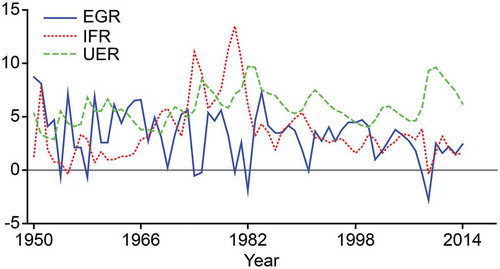
The crests and troughs for the inflation rate are in contrast to those for economic growth. Between the late 1970s and the early 1980s, there was a high unemployment rate and the amplitudes clearly reflect global stagflation. In 2009, the U.S. economy slipped into a large trough, while unemployment peaked. Fortunately, inflation did not increase. Although there were many potential causes of stagflation in the 65-year period between 1950 and 2014, including the global oil crisis, we examine the impact of government-led rigid welfare (LGSP) on stagflation.

Cointegration bounds testing

We use an autoregressive distributed lag (ARDL) bounds testing approach to cointegration that was developed by Pesaran Shin, and Smith (2001) to examine the effects of the LGSP on stagflation. Compared with other cointegration procedures (Engle and Granger 1987; Johansen 1988; Johansen and Juselius 1990), the ARDL bounds testing approach has several advantages, including: 1) the regressors are not restricted when they have pure I(0), pure I(1) or mutual cointegration; 2) both long- and short-term relationships are easy to investigate and 3) in small samples, cointegration is more difficult to obtain (Brahmasrene and Jiranyakul 2009; Adetunji 2011; Lamotte et al. 2013).

However, the regressors remain restricted under I(2) in the bounds testing approach. Thus, we first used the Augmented Dickey–Fuller (ADF) test that was suggested by Dickey and Fuller (1979, 1981) to examine the stationarity of the time series data (LGSP, EGR, IFR and UER). After this condition was met, we constructed several conditional error-correction models (ECMs) to perform cointegration bounds testing, with Case I (no intercept; no trend), Case III (unrestricted intercept; no trend) and Case V (unrestricted intercept; unrestricted trend) provided by Pesaran, Shin, and Smith (2001), which are shown in Equations 1, 2 and 3.

(1) $d{Y}_{j,t}={\pi }_{j,Y}{Y}_{j,t-1}+{\pi }_{j,X}{X}_{t-1}+\sum _{i=1}^{p_j-1}{{\psi }_j}^{\prime }d{Z}_{j,t-i}+{{\omega }_j}^{\prime }d{X}_t+{\epsilon }_{j,t},$(1)

(2) $d{Y}_{j,t}=C_{j0}+{\pi }_{j,Y}{Y}_{j,t-1}+{\pi }_{j,X}{X}_{t-1}+\sum _{i=1}^{p_j-1}{{\psi }_j}^{\prime }d{Z}_{j,t-i}+{{\omega }_j}^{\prime }d{X}_t+{\epsilon }_{j,t},$(2)

(3) $d{Y}_{j,t}=C_{j0}+C_{j1}{T}_j+{\pi }_{j,Y}{Y}_{j,t-1}+{\pi }_{j,X}{X}_{t-1}+\sum _{i=1}^{p_j-1}{{\psi }_j}^{\prime }d{Z}_{j,t-i}+{{\omega }_j}^{\prime }d{X}_t+{\epsilon }_{j,t},$(3)

where:

$\begin{array}{c}{X}_t=LGS{P}_{t;}\\ Y_{j,t}=EG{R}_{t,}IF{R}_{t}orUE{R}_t,j=1,2,3.\\ Z_{j,t}={\left(Y_{j,t},X_t\right)}^{{ }^{\prime }};\end{array}$

• p_j denotes the lag;

  d is the difference operator;

  t denotes the year;

  C_j0 is the intercept;

  T_j represents the trend;

  ε,_j,t ∈ (0, σ²), is white noise;

  C_j1, π_jy, π_jx, ψ_j^’ and ω_j’ are coefficients;

The null hypothesis is H₀: π_j,Y = π_j,X = 0. The F-statistic for cointegration is denoted as F(EGR/LGSP), F(IFR/LGSP) or F(UER/LGSP). Pesaran, Shin, and Smith (2001) tabulated two sets of critical values: I(0) and I(1). When the F-statistic is less than the lower bound I(0), the null hypothesis (H₀) of no cointegration cannot be rejected. When the F-statistic exceeds the upper bound I(1), H₀ can be rejected and there is a relationship across levels or variable cointegration. When the value of the F-statistic falls within the bounds of I(0) and I(1), we cannot make a conclusive inference.

The ARDL long-run and short-run relationship

After cointegration was tested (EGR and LGSP, IFR and LGSP, UER and LGSP), we examined (p_j+1)¹⁺¹ ARDL models and identified the ARDL models with optimal lags based on the Akaike Information Criterion (AIC), Schwarz Bayesian Criterion (SBC), and Hannan Quinn Criterion (HQC), which are shown in Equation 4.

(4) ${\varphi }_j(L,p_{j,0})Y_{j,t}=(Cons{t}_j)+(T_j)+{\theta }_j(L,q_{j,1})X_t+{\mu }_{j,t},$(4)

$where:\varphi (L,p_{j,0})=1-{\varphi }_{j1}L-{\varphi }_{j2}{L}^2-\cdots -{\varphi }_{p_{j,0}}{L}^{p_{j,0}},$

$\theta (L,q_{j,1})={\theta }_{j0}+{\theta }_{j1}L+{\theta }_{j2}{L}^2+\cdots +{\theta }_{q_{j,1}}{L}^{q_{j,1}}.$

ARDL (p_j,0, q_j,1) is chosen with optimal lags p_j,0, and q_j,1, and L is the lag operator such that LⁱX_t = X_t-i. Based on the above cointegration bounds testing, (Const_j) refers to no or unrestricted intercepts and (T_j) refers to no or unrestricted trends. Next, by adding and subtracting items, we can achieve long- and short-term relationships. The long-term equation is shown in Equation 5 and the short-term dynamic equation with an error-correction term is shown in Equation 6:

(5) $Y_j=(INP{T}_j)+(Tren{d}_j)+{\beta }_j\cdot X+v_j,$(5)

$where:INP{T}_j=Cons{t}_j/\varphi (1,p_{j,0});$

$Tren{d}_j=T_j/\varphi (1,p_{j,0});$

${\beta }_j=\theta (1,q_{j,1})/\varphi (1,p_{j,0}).$

(6) $\begin{array}{rl}d{Y}_{j,t}=& (dINP{T}_j)+(dTren{d}_j)-\sum _{i=1}^{p_{j,0}-1}\sum _{g=i+1}^{p_{j,0}}{\varphi }_g\cdot d{Y}_{j,t-i}\\ & +\theta (0,q_{j,1})\cdot d{X}_t-\sum _{i=1}^{q_{j,1}-1}\sum _{g=i+1}^{q_{j,1}}{\theta }_g\cdot d{X}_{j,t-i}\\ & -\varphi (1,p_{j,0})\cdot ecm(-1)+u_{j,t}\end{array},$(6)

$\begin{array}{l}where:ec{m}_{j,t}=Y_{j,t}-(INP{T}_j)-(Tren{d}_j)\\ -{\beta }_{j,t}\cdot X_t+v_{j,}{\hspace{0.17em}}_t.\end{array}$

Analysing the long- and short-term relationships allows us to investigate the impact of X(LGSP) on Y_j (EGR, IFR and UER) – in other words, the influence of government-led rigid welfare (LGSP) on stagflation – using an empirical bounds testing approach.

IV. Results

We used an ADF test to examine the LGSP, EGR, IFR and UER. All variables were in I(2). Thus, we used conditional error-correction models to compute the F-statistics to test the cointegration relationships in which the maximum lag length, p, is 2. The results of the bounds F-tests are shown in Table 1.

Table 1. Results of the bounds F-tests.

	Case I	Case III	Case V
F(EGR/LGSP)	0.95451	8.9706***	8.4331**
F(IFR/LGSP):	7.3803***	7.3563**	10.4541***
F(UER/LGSP):	12.9440***	4.1189	1.2923
Lower I(0)–upper I(1)
1% level:	4.81–6.02	6.84–7.84	8.74–9.63
5% level:	3.15–4.11	4.94–5.73	6.56–7.30
10% level:	2.44–3.28	4.04–4.78	5.59–6.26

Notes: **denotes significance at the (α = 0.05) level; and ***denotes significance at the (α = 0.01) level. Asymptotic critical values are obtained from Pesaran, Shin, and Smith (2001): Table CI(i) Case I, no intercept and no trend; Table CI(iii) Case III, unrestricted intercept and no trend; and Table CI(V) Case V, unrestricted intercept and unrestricted trend.

When the F-statistics exceed the upper bound I(1), there are cointegration relationships in the variables. Thus, Cases III and V can be used to analyse the relationship between EGR and LGSP; Cases I, III and V are analysed for IFR and LGSP; and Case V is analysed for UER and LGSP. Using the above ARDL bounds testing approach to cointegration (Equation 4–6), we obtained the long- and short-run relationships. However, several F and T-Ratio statistics were not significant. Thus, we eliminated several options (not shown in this article) and used Case III to analyse the nexus between EGR and LGSP, Case V to analyse IFR and LGSP, and Case I to analyse UER and LGSP.

Based on the SBC, we determine the ARDL model with optimal lags, ARDL(0,2), to display the relationship between EGR and LGSP. As shown in Equations 7–9, ARDL(1,1) is for IFR and LGSP, and ARDL(2,1) is for UER and LGSP.

(7) $\begin{array}{rl}EGR& =-32.4058\ast LGSP[.000]+39.7842\ast \\ & LGSP(-1)[.000]-8.0221\ast LGSP(-2)[.027]\\ & +8.7374[.000]\end{array},$(7)

(F-Stat. F(3,59) = 17.4819[0.000]),

(8) $\begin{array}{rl}IFR=& 0.53438\ast IFR(-1)[.000]+15.0758\ast \\ & LGSP[.004]-12.7072\ast LGSP(-1)[.010]\\ & -5.5496[.027]-0.20378\ast Trend[.047]\end{array},$(8)

(F-Stat. F(4,58) = 30.9340[0.000]),

(9) $\begin{array}{rl}UER=& 0.93685\ast UER(-1)[.000]-0.19388\ast \\ & UER(-2)[.042]+10.4951\ast LGSP[.000]\\ & -10.3717\ast LGSP(-1)[.000]\end{array},$(9)

(F-Stat. F(3,59) = 73.5629[0.000]).

The F-statistics from the ARDL regression were satisfactory. The probability of the null hypothesis of all-zeros is [0.000]. Furthermore, for the T-Ratio [Prob], all coefficients were significant at the α = 0.05 level. Thus, the three ARDL models are well-established. Hence, based on the above ARDL models, we can identify long-run slope relationships and the short-run error correcting relationships between government social benefit expenditures (LGSP) and stagflation (EGR, IFR and UER). The results from this analysis in the U.S. are shown in Tables 2^{Table 3}–4.

Table 2. The ARDL long-run relationships (EGR and LGSP).

The ARDL long-run relationship (dependent variable EGR):
Regressor	Coefficient	Standard Error	T-Ratio[Prob]
LGSP	−0.64379	0.13243	−4.8614[0.000]
INPT	8.7374	0.94754	9.2211[0.000]

Note: The results were calculated using the Microfit 5.0 software, which was developed by professors Pesaran, M. H. and Pesaran, B.@ Oxford University Press.

Table 3. The long- and short-run ARDL relationships (IFR and LGSP).

Regressor	Coefficient	Standard error	T-Ratio[Prob]
The ARDL long-run relationship (dependent variable IFR):
LGSP	5.087	1.7985	2.8285[0.006]
INPT	−11.9187	4.1936	−2.8421[0.006]
TREND	−0.43765	0.16999	−2.5746[0.013]
The ARDL short-run relationship or the Error Correction Model (dependent variable dIFR):
dLGSP	15.0758	4.9689	3.0341[0.004]
dTREND	−0.20378	0.10023	−2.0331[0.047]
ecm(−1)	−0.46562	0.1075	−4.3314[0.000]
Additional temporary variables:
dIFR = IFR-IFR(−1)
dLGSP = LGSP-LGSP(−1)
dTREND = TREND-TREND(−1)
ecm = IFR −5.0870*LGSP + 11.9187*INPT + 0.43765*TREND
(F-Stat. F = 6.8009[0.001])

Note: The results were calculated using the Microfit 5.0 software, which was developed by professors Pesaran, M. H. and Pesaran, B. @ Oxford University Press.

Table 4. The long- and short-run ARDL relationships (UER and LGSP).

Regressor	Coefficient	Standard error	T-Ratio[Prob]
The ARDL long-run relationship (dependent variable UER):
LGSP	0.48022	0.14582	3.2931[0.002]
The ARDL short-run relationship or the Error Correction Model (dependent variable dUER):
dUER1	0.19388	0.093444	2.0749[0.042]
dLGSP	10.4951	1.5079	6.9599[0.000]
ecm(−1)	−0.25703	0.05662	−4.5396[0.000]
Additional temporary variables:
dUER = UER-UER(−1)
dUER1 = UER(−1)-UER(−2)
dLGSP = LGSP-LGSP(−1)
ecm = UER −0.48022*LGSP
(F-Stat. F = 30.2888[0.000])

Note: The results were calculated using the Microfit 5.0 software, which was developed by professors Pesaran, M. H. and Pesaran, B. @ Oxford University Press.

In the long run, the elasticity of LGSP contributing to EGR is −0.64379, and its T-Ratio[Prob] is −4.8614[0.000]. The EGR negatively responds to the LGSP in the U.S. over the 65-year period from 1950 to 2014 and the T-Ratio for LGSP is significant at the α = 0.01 level. The intercept coefficient INPT is 8.7374, and its T-Ratio is satisfactory (9.2211[0.000]). However, the elasticity of LGSP contributing to IFR is 5.087, and its T-Ratio[Prob] is 2.8285[0.006]. Thus, IFR is positively associated with LGSP in the U.S. During the same time period, the LGSP increases the IFR. The T-Ratios for the coefficients in that regression model are satisfactory and significant at the α(0.01) level. In addition, the UER is positively related to the LGSP. The elasticity coefficient is 0.48022, and the T-Ratio[Prob] is 3.2931[0.002], which is significant at the α = 0.01 level. Thus, the LGSP contributed to stagflation in the U.S. over the 65-year period that is examined.

Moreover, the first ARDL model has no lagged dependent variable EGR. Thus, there is no short-run error correction between EGR and LGSP, and it is thus not displayed here. The dLGSP coefficient is 15.0758 for the dependent variable, dIFR. Thus, dLGSP is positively related to dIFR. LGSP changes in the same direction as IFR. In addition, with respect to the dependent variable dUER, the dLGSP coefficient is 10.4951, which suggests that LGSP is consistent with UER in the U.S. In the short-run ARDL relationship, the F- and T-statistics are all satisfactory. The F-statistics for the two regression models are 6.8009[0.001] and 30.2888[0.000], and the Prob(F-statistics) < α(0.01); thus, the null hypothesis, β_j = 0, is rejected. The Prob(T-Ratio) are also < α(0.05). As expected, all the Error Correction Terms (ecm(−1)) are negative, −0.46562 and −0.25703, which demonstrates the adjusting speeds of LGSP on IFR and UER in the long-run equilibrium relationships. Thus, the short-run ARDL models are well established.

The results clearly show that LGSP restrains EGR and is in accordance with IFR and UER in the U.S. over the past 65 years. The counterinfluences of LGSP on EGR as well as IFR and UER reflect monetarism, in that government expenditures may increase the money supply to an extent. When the growth in the money supply does not stimulate growth in the economy, it may result in inflation. In addition, it is possible that increased spending on welfare may increase laziness, which might result in high unemployment rates. Empirically, rigid welfare is one of the causes of stagflation in the U.S. If ignored, an over-dependence on welfare might lead to stagflation again.CUSUM and CUSUMSQ

The empirical ARDL models required further confirmation. We used the cumulative sum of recursive residuals (CUSUM) and cumulative sum of the squares of recursive residuals (CUSUMSQ) methods to test the stability of the models, and the results are shown in Figure 2 (a:EGR_LGSP_CUSUM; b: EGR_LGSP_CUSUMSQ; c:IFR_LGSP_CUSUM; d: IFR_LGSP_CUSUMSQ: e: UER_LGSP_CUSUM; f: UER_LGSP_CUSUMSQ).

Figure 2. CUSUM and CUSUMSQ values.

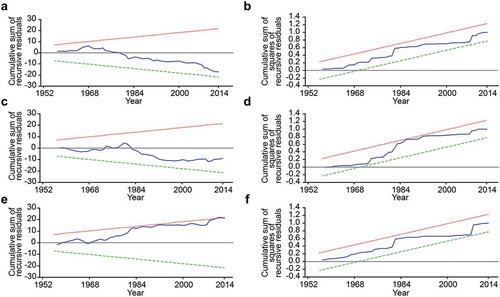
The straight lines represent the critical bounds at a 5% significance level. When CUSUM or CUSMSQ move beyond the two straight lines, we reject the hypothesis of stability and have evidence of structural instability in the estimated model. However, based on our ARDL models, all CUSUM and CUSUMSQ values for the forecasted residuals for LGSP on EGR, IFR and UER are within the standard error bands. Thus, we accept the stability of the models. Because there is no break point, the models are effective with stable recursive residuals that show the counter influence of LGSP on EGR, IFR and UER, i.e. the effect of social benefit expenditures on stagflation. We believe that these stable properties could be valuable to policymakers in the U.S.

V. Conclusion

The purpose of this article was to explore the impact of social benefit expenditures on stagflation in the U.S. over a 65-year period from 1950 until 2014. Stagflation is a terrible economic malaise that should of course be avoided. We empirically investigated rigid welfare LGSP as a potentially new cause of stagflation. This research is novel because it probed the influence of LGSP and found long- and short-term relationships with EGR, IFR and UER, i.e. with stagflation.

We used an ADRL bounds testing approach to cointegration that was developed by Pesaran, Shin, and Smith (2001) to examine those relationships. We showed that LGSP produces a negative effect on EGR in the U.S. The long-run slope coefficient was −0.64379, and all other regressors (T-Ratio[Prob]) were significant at the α = 0.01 level. In addition, the CUSUM and CUSUMSQ values for the recursive residuals in the estimated model showed stability. Thus, government social benefit expenditures block economic growth, which has been shown in other countries characterized by high well-being.

By contrast, IFR and UER respond positively to LGSP in the U.S. The long-run slope coefficients are 5.087 and 0.48022, and the short-run dynamic coefficients are 15.0758 and 0.19388, whereas the speed of adjustment is −0.46562 and −0.25703. All regressors (T-Ratio[Prob]) were significant at the α = 0.05 level, and F-statistics were significant at the α = 0.01 level. Moreover, the CUSUM and CUSUMSQ values for the recursive residuals were examined for stability. Thus, we show that monetarism in the form of governmental expenditures can, to an extent, increase the money supply, thus leading to inflation, and drive people towards laziness in terms of unemployment.

Thus, as one cause of stagflation, the social benefit expenditure LGSP has an impact on stagflation. Because LGSP is rigid and difficult to reduce, increased welfare burdens could lead to stagflation. This finding is important for U.S. policymakers and can inform governments in other countries that are characterized by high levels of well-being.

Disclosure statement

No potential conflict of interest was reported by the authors.

References

- Adetunji, B. M. 2011. “A Bound Testing Analysis of Wagner’s Law in Nigeria: 1970–2006.” Applied Economics 43 (21): 2843–2850. doi:10.1080/00036840903425012.
- Herbst, A. F., J. S. K. Wu, and C. P. Ho. 2014. “Quantitative Easing in an Open Economy-Not a Liquidity but a Reserve Trap.” Global Finance Journal 25 (1): 1–16. doi:10.1016/j.gfj.2014.03.004.
- Barsky, R. B., and L. Kilian. 2000. “A Monetary Explanation of the Great Stagflation of the 1970s.” NBER Working Paper No. 7547. http://www.nber.org/papers/w7547
- Brahmasrene, T., and K. Jiranyakul. 2009. “Capital Mobility in Asia: Evidence from Bounds Testing of Cointegration Between Savings and Investment.” Journal of the Asia Pacific Economy 14 (3): 262–269. doi:10.1080/13547860902975077.
- Dickey, D. A., and W. A. Fuller. 1979. “Distribution of the Estimators for Autoregressive Time Series with a Unit Root.” Journal of the American Statistical Association 74 (366a): 427–431. doi:10.1080/01621459.1979.10482531.
- Dickey, D. A., and W. A. Fuller. 1981. “Likelihood Ratio Statistics for Autoregressive Time Series with a Unit Root.” Econometrica 49 (4): 1057–1072. doi:10.2307/1912517.
- Nelson E., and K. Nikolov. 2004. “Monetary Policy and Stagflation in the UK.” Journal of Money, Credit and Banking 36 (3): 293–318. doi:10.1353/mcb.2004.0058.
- Engle, R. F., and C. W. J. Granger. 1987. “Co-integration and Error Correction: Representation, Estimation and Testing.” Econometrica 55 (2): 251–276. doi:10.2307/1913236.
- Forder, J. 2010. “Friedman’s Nobel Lecture and the Phillips Curve Myth.” Journal of the History of Economic Thought 32 (3): 329–348. doi:10.1017/S1053837210000301.
- Geanakoplos, J., and P. Dubey. 2010. “Credit Cards and Inflation.” Games & Economic Behavior 70 (2): 325–353. doi:10.1016/j.geb.2010.02.004.
- Jiménez-Rodríguez, R., and M. Sánchez. 2010. “Oil-Induced Stagflation: A Comparison across Major G7 Economies and Shock Episodes.” Applied Economics Letters 17 (15): 1537–1541. doi:10.1080/13504850903035923.
- Johansen, S. 1988. “Statistical-Analysis of Cointegration Vectors.” Journal of Economic Dynamics and Control 12: 231–254. doi:10.1016/0165-1889(88)90041-3.
- Johansen, S., and K. Juselius. 1990. “Maximum Likelihood Estimation and Inference on Cointegration: With Applications to the Demand for Money.” Oxford Bulletin of Economics & Statistics 52 (2): 169–210. doi:10.1111/j.1468-0084.1990.mp52002003.x.
- Kilian, L. 2008. “A Comparison of the Effects of Exogenous Oil Supply Shocks on Output and Inflation in the G7 Countries.” Journal of the European Economic Association 6 (1): 78–121. doi:10.1162/JEEA.2008.6.1.78.
- Kyrtsou, C., A. G. Malliaris, and A. Serletis. 2009. “Energy Sector Pricing: On the Role of Neglected Nonlinearity.” Energy Economics 31 (3): 492–502. doi:10.1016/j.eneco.2008.12.009.
- Lamotte, O., T. Porcher, C. Schalck, and S. Silvestre. 2013. “Asymmetric Gasoline Price Responses in France.” Applied Economics Letters 20 (5): 457–461. doi:10.1080/13504851.2012.714063.
- Bonatti, L., and A. Fracasso. 2013. “Hoarding of International Reserves in China: Mercantilism, Domestic Consumption and US Monetary Policy.” Journal of International Money and Finance 32: 1044–1078. doi:10.1016/j.jimonfin.2012.08.007.
- McDonald, B. D., and D. R. Miller. 2010. “Welfare Programs and the State Economy.” Journal of Policy Modeling 32 (6): 719–732. doi:10.1016/j.jpolmod.2010.08.003.
- Pereira, A. M., and J. M. Andraz. 2015. “On the Long-term Macroeconomic Effects of Social Spending in the United States.” Applied Economics Letters 22 (2): 132–136. doi:10.1080/13504851.2014.929620.
- Pesaran, M. H., Y. Shin, and R. J. Smith. 2001. “Bounds Testing Approaches to the Analysis of Level Relationships.” Journal of Applied Econometrics 16 (3): 289–326. doi:10.1002/jae.616.
- Phillips, A. W. 1958. “The Relation Between Unemployment and the Rate of Change of Money Wage Rates in the United Kingdom, 1861–1957.” Economica 25 (100): 283–299. doi:10.1111/j.1468-0335.1958.tb00003.x.
- Vanags, A., and M. Hansen. 2008. “Stagflation in Latvia: How Long, How Far, How Deep?” Baltic Journal of Economics 8 (1): 5–28. doi:10.1080/1406099X.2008.10840443.
- Wahid, A. N. M. 2000. “Stagflation and Stability of the Keynesian Consumption Function: An Empricial Analysis.” Applied Economics Letters 7 (6): 357–359. doi:10.1080/135048500351276.
- Zandi, M. 2009. Financial Shock. Upper Saddle River: FT Press.
- Shipchandler, Z. E 1982. “Keeping down with the Joneses: Stagflation and Buyer Behavior.” Business Horizons 25 (6): 32–38. doi:10.1016/0007-6813(82)90006-4.