Estimating the household consumption function in Saudi Arabia: an error correction approach

ABSTRACT

We estimate a micro-founded life-cycle consumption model for Saudi Arabia over the period 1970–2017 using error correction model procedures. Dynamic adjustments are significant, and both income and wealth are found to have significant effects, with a long-run marginal propensity to consume out of the income of 0.95 and out of the wealth of 0.06. The sensitivity of consumption to income and wealth, as well as the estimated short-term effects of price and real interest rate, are consistent with the rapidly growing Saudi economy. By capturing the key determinants of the life-cycle model, our approach is useful for the design of macroeconomic policy. We estimate the impact of the recent VAT reform.

KEYWORDS:

• Consumption function
• life-cycle hypothesis
• marginal propensity to consume
• wealth effect
• cointegration
• Saudi Arabia

JEL CLASSIFICATION:

• C12
• C22
• E21

I. Introduction

There have been several important economic policy changes in the Kingdom of Saudi Arabia, such as energy price reforms, the introduction of a value-added tax (VAT) in 2018 and a new fiscal stimulus package. In the context of macroeconomic analysis, capturing the behaviour of private consumption is of crucial interest for both fiscal and monetary authorities. The design of an appropriate national fiscal policy requires understanding private consumption patterns. Consumption growth is at the root of real growth and saving is at the root of investment growth. In addition, very rapid economic growth can lead to inflationary pressures. Given that the ultimate goal of economic policies is to spur economic growth and welfare, an accurate and robust estimation of the consumption behaviour should be a helpful, perhaps even a necessary, tool for policymakers.

This paper aims to make a new contribution to the literature, estimating a fully micro-founded life cycle consumption model for Saudi Arabia, using data for consumption, disposable income, interest rate, and wealth. The analysis of the macro consumption function has two lines of interest: i) macroeconomic compatibility of aggregate savings and consumption patterns with the objectives of an economic growth policy, and ii) individual intertemporal behaviour in the life cycle framework, including institutional analysis of market imperfections, liquidity constraints, and asymmetric information (Kaplan and Violante 2010; Fisher, Huh, and Otto 2012). In addition, the empirical analysis of consumption behaviour has separately estimated income effects and wealth effects. The income effect is the direct impact on consumption of a variation in income. The wealth effect is the response of consumption when the consumer perceives a change in his wealth and decides to liquidate a part of it to increase consumption (in the case of a positive change in wealth) or to reduce consumption to restore the desired level of wealth (in the case of a negative change in wealth). The wealth effect on consumption can be substantially different from the income effect, because it is more related to consumers’ perceptions of expectations and fluctuations of the value of real and financial assets and can vary across different economies. Studies for advanced economies have highlighted that the wealth effect is lower in the Euro area than in the United States (Slacalek 2009; Sousa 2008, 2009) and that persistent responses to shocks imply that the long-run effect of wealth is significantly larger than its short-run effect.

The macro empirical literature uses aggregate time series variables to specify a dynamic representation of short-term adjustments and a long-term structural relation using an error correction model (ECM) representation. The empirical results show differences between advanced and emerging countries (Peltonen, Sousa, and Vansteenkiste 2012) and between two types of consumers: those who can freely borrow and those who are unable to borrow (for whatever reason). The former is more able to smooth and adapt their behaviour to sudden shocks, while the latter are forced by sudden shocks to adapt their consumption behaviour (Attanasio and Pistaferri 2016 and Attanasio and Weber 1993). Differences in life-cycle consumption patterns are explored in terms of overconfidence behaviour by Caliendo and Kevin X.D. (2008). Sapci (2017) argues that a lower volatility of financial system yields higher consumption smoothing.

A vast literature (as discussed in Jappelli and Pistaferri 2010) analysing developed economies shows a marginal propensity to consume (MPC) ranging between 0.5 and 0.9. These estimations take into account predictable and unpredictable income changes, precautionary savings, credit, and insurance market instruments available to consumers. Recent work (Xuan, Kim, and Kim 2019) shows evidence of faster adjustment of consumption to changes in permanent income, than in previous work. So far, scarce attention has been devoted to the determinants of such aggregate patterns in emerging economies.

The rest of the paper is organized as follows: Section 2 surveys the existing literature, Section 3 provides a review of the data and methodology, and Section 4 summarizes the empirical results. Section 5 concludes the paper.

II. What we learn from the literature

After Keynes John’s (1936) absolute-income hypothesis according to which consumption grows at a fraction of current income and Duesenberry’s (1949) relative-income hypothesis according to which current levels of consumption are also driven by past levels of consumption, the theory of consumption has been enriched by Modigliani and Brumberg (1954) Life-Cycle Hypothesis (LCH). LHC explains aggregate consumption from a representation of individual behaviour, assuming a specification of a multi-period utility maximization. Aggregate consumption then depends on income, interest rate, wealth, and the age of the agent. Friedman (1957) provided the permanent-income hypothesis (PIH) to account for empirical anomalies in the data for prior hypotheses. Later, Hall Robert (1978) has applied rational expectations to both the LCH and the PIH. Several papers were then conducted to explore the consumption function for developed economies (Muellbauer 1994; Church, Smith, and Wallis 1994; Hendry 1994; Muellbauer and Lattimore 1995; Craigwell and Rock 1995; Fagan, Henry, and Mestre 2005; Smets and Wouters 2003; Davis and Palumbo 2001; Sapci 2017; Ismail and Rashid 2013). Some studies which have also included wealth effects are: Patterson (1991); Rossi and Visco (1994), Fisher, Huh, and Otto (2012); MacDonald, Mullineux, and Sensarma (2011); for Turkey, Aydede (2008).

The main lesson from the literature is that an individual consumer takes into account not only his current income but also his expectation of future income streams, his accumulated and expected wealth, and an appropriate interest rate for discounting future income. In addition, consumers may decide to absorb short-term income fluctuations, which may yield an increase in savings to postpone current consumption or a decrease in saving to maintain current consumption levels at the expense of future consumption. The bulk of the literature is on developed economies. Less attention has been paid to developing economies. Research on Saudi Arabia is limited but includes Al-Bashir (1977) with data referring to the 1960s; Tawi (1984); Ibrahim (2014); and Algaeed (2016). Tawi (1984) estimated several specifications, from a simple Keynesian consumption function to a permanent-income consumption function. The very low estimated MPC (0.40) is justified by the number of foreign workers who save a high proportion of their income, combined with the fact that many basic goods and health and education services are subsidized. These results are of limited use as the estimation is static. Ibrahim (2014) also finds a very low MPC of around 0.4 and Algaeed (2016) finds only monetary effects on consumption. Alsamara et al. (2017) find evidence of a stable macro money demand function for Saudi Arabia. Hasanov, Joutz, and Mikayilov (2018) estimate consumption in an annual macro model for Saudi Arabia from 1997–2015, estimating an MPC of around 0.7. In summary, the previous estimation of the MPC in Saudi Arabia is in the range 0.4–0.7. We note that one implication of the economic theory is that the MPC is higher in low wealth countries (Carroll, Slacalek, and Tokuoka 2014) and in emerging economies. Also, the MPC depends on the population age composition of the economy, as the LCH predicts lower MPCs in middle age, with higher consumption rates among young people. In this sense, the MPC in the Saudi economy, which has a young population, should be higher than that of advanced economies because the population of advanced economies is, on average, older than in the Kingdom. The MPC in Saudi Arabia should be higher than in many emerging countries because incomes in emerging economies are, on average, lower than in the Kingdom.

In addition, Saudi consumers have taken a more cautious attitude towards the local stock market (Tadawul) after the turbulence induced by the Great Recession . Jawadi, Jawadi, and Cheffou (2018) find a positive impact of the stock market on the expectation for economic growth in the framework of Vision 2030. Khalifa, Hammoudeh, and Otranto (2014), Naifar and Al Dohaiman (2013) and Finta, Frijns, and Tourani-Rad (2019) discuss the Saudi Stock market volatility and the spillovers from the oil market.

To the best of our knowledge, our proposed dynamic consumption function for Saudi Arabia, following the seminal work of Ando and Modigliani (1963),¹ is the first attempt to examine the MPC out of income in a fully theoretical life cycle dynamic model.

III. Data and methodology

Data

Our econometric analysis of the household’s consumption function of Saudi Arabia is micro-founded and based on the traditional linear approximation of the Ando-Modigliani life cycle model.

The data used are taken from Saudi Arabia’s General Authority for Statistics (GaStat) and the Saudi Arabian Monetary Authority’s (SAMA’s) yearly published statistics from 1970–2017. We denote the real consumption with c, the rate of change of prices with π, the real interest rate with r, the real income with y, the real wealth with w and savings with s = y-c.

The choice of the empirical variables is guided by the principle of using official data that are clearly identifiable and recoverable from the published statistics, as is common practice in macro-econometric models (for instance, Cicowiez and Lofgren 2017; Vitek 2018). We take the private final consumption expenditure, in 2010 prices, from the national accounts, defined as c. We take as income y the non-oil gross domestic product (GDP) in million Saudi Arabian Riyals (SAR), in 2010 prices (non-oil GDP is defined by the national income accounts). We construct the wealth variable w as the sum of financial wealth approximated by the broad money supply (M3) and the market capitalization of the Tadawul stock market, using published GaStat data. We have followed the methodology of constructing the financial wealth of the household sector used by the International Monetary Fund (IMF (2006) and the ECB (2016)² In the recent period, there has been a phase of relatively high growth of non-oil GDP in real terms (above 6%) from 2008 to 2014 and a second phase of lower growth rate in 2015–2017. The real private consumption growth rate has generally been higher than the non-oil GDP growth rate, with exceptions only in 2010, 2011 and 2013.

Figures 1 and 2 show the long term-trend in consumption and income and the consumption/income ratio. Note that in the last 20 years, real consumption and income increased three times. The big fluctuation of the consumption/income ratio in the 1970s is due to the sudden increase in non-oil GDP in 1974–75, which was followed by a sluggish increase in private consumption. The consumption/income ratio was more stable after 1982.

Figure 1. Consumption and income (billion real SAR).

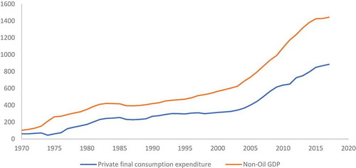
Figure 2. Consumption to income ratio – Average propensity to consume.

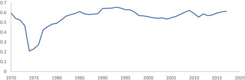
Consumption growth slowed from 2016 to 2017, following a fall in GDP. The combined result has been a slight increase in consumption/income ratio since 2015.

Methodology

Our empirical representation of the consumption function assumes that the relevant driver is the income attributable to the non-oil sector. We assume that the relevant wealth concept is the financial wealth (we do not consider real wealth, because it is less clear what type of effect the variation in housing prices can have on current consumption). The inflation rate π is defined as the rate of change of the consumer price index (CPI). The real interest rate r is defined as the short-term rate on USD deposits deflated with the rate of change of the consumer price index: r = (1+ r_USD)/(1 + π). Empirical macroeconomic evidence of the typical life cycle model remains a cornerstone of the explanation of macroeconomic systems, both from a positive analysis viewpoint John (1994) and from a normative analysis viewpoint. We follow the usual simplifying assumptions which allow us to specify a linear consumption function, where the savings rate depends on the interest rate (intertemporal substitution effect), on the wealth-income ratio (capturing the optimizing life-cycle behaviour), and on a set of other structural variables (for example, socio-economic variables, Bick and Cho 2013).

Formally, let us define labour income and total disposable income as y^l and y, respectively, (noting that y = y^l+rw), the growth rate in the steady state of real income as g, wealth as w, and interest rate as r, while z is a vector of other relevant structural determinants. The simple consumption function:

(1) $c=a{y}^l+\beta w$(1)

where α and β are approximately constant coefficients can be rewritten, using y = y^l+rw to capture the life-cycle hypothesis:

(2) $c=a\left(z\right)y+\beta \left(r,g\right)w$(2)

where the coefficients are now more complex: α (z) captures aggregation of the structure of preferences, productivity growth, population growth and other heterogeneous socio-demographic influences and β (r,g) captures productivity growth and interest effects (Modigliani 1986). The linearization of Equation (2) for empirical estimation, around long-run equilibrium values of g, r and w/y, allows to obtain an equation where the relevant propensities to consume are recoverable from the empirical estimation in a linear relation, as follows:

(3) $c/y=a_0+\sum a_j{z}_j+b_{1}r+b_{2}g+d\left(w/y\right)$(3)

Equation (3) is an approximate relation, where the heterogeneous socio-demographic determinants (variables z_j) could capture aggregation effects which may not be justifiable, based on rigorous theoretical specification of the individual life-cycle model. On this point see also: Ostry and Levy1995) who investigate the effect of heterogeneity of individual responses to future income uncertainty (the idea of ‘saving for a rainy day’) as a shifting factor of the aggregate result and Sarel 1995) who introduces labour productivity changing with the age structure of the population as determinant of macroeconomic growth.

With these caveats, we consider Equation (3) as an approximation of the long run equilibrium representation of the relation among consumption income and wealth in the empirical estimation, which has been extensively estimated in the literature and in the ECM form. For instance, applications to the USA, the UK, some Nordic European countries, Japan and Australia are provided by John (1994) Church, Smith, and Wallis (1994); and David (1994), who review some twenty years of econometric estimation evidence³

IV. Empirical results

We conducted a preliminary integration analysis of consumption, income, wealth, cpi and interest rate (Table 1) to avoid the risk of estimating spurious correlations. We used the Augmented Dicky-Fuller (ADF) test (Dickey and Fuller 1979) and the Weighted Symmetric test (WS)⁴ (Pantula, Gonzalez-Farias, and Fuller 1994). Notice that the period is rather short and thus the results (Johansen ML method) are weak, due to scarce degrees of freedom, although reasonable.

Table 1. Stationarity test results.

	ADF test (n. lags)		WS test (n. lags)
	1970–2017	1982–2017	1970–2017	1982–2017
Panel A – variables in levels
c none	−1.267 (3)	−1.050 (2)	−0.657 (3)	−0.396 (3)
Const	0.36 (3)	0.755 (2)	−1.299 (3)	2.970 (3)
Trend	1.66 (3)	1.678 (2)
y none	−2.075 (9)	−2.548 (9)	−0.469 (9)	2.699 (9)
const	1.297 (9)	2.281 (9)	−1.243 (9)	0.985 (9)
trend	2.536 (9)	2.371 (9)
w none	−1.473 (8)	−1.252 (9)	−0.254 (3)	−0.314 (3)
const	−0.461 (8)	1.174 (9)	−4.465* (3)	−2.122 (3)
trend	1.976 (8)	2.054 (9)
r none	−3.952* (3)	−1.495 (10)	−2.617 (2)	−1.565 (10)
const	4.779* (3)	1.399 (10)	13.16* (2)	9.564* (10)
trend	−3.736* (3)	−1.581 (10)
cpi none	−2.73 (4)	0.863 (10)	−0.85 (9)	−0.71 (3)
const	2.64 (4)	−0.914 (10)	11.51* (9)	26.41* (3)
trend	−2.51 (4)	1.276 (10)
	1970–2017	1982–2017
Panel B – variables in log changes and interest rate
dln(cpi) none	−3.243* (2)	−4.112* (10)
const	2.331 * (2)	−2.300* (10)
r none	−3.952* (3)	−1.495 (10)
const	4.779* (3)	1.399 (10)
dln(c) none	−4.535* (3)	−2.592* (2)
const	3.568* (3)	2.273 (2)
dln(y) none	−5.769* (3)	−3.304* (2)
const	2.594* (3)	3.058* (2)
dln(w) none	−2.680* (3)	−1.996 (2)
const	2.454 (3)	7.787* (2)

Note: ADF: Augmented Dicky-Fuller; WS: Weighted Symmetric; n. lags: number of lags is determined according to the Akaike information criterion; *: test significance at 5% level.

We tested the stationarity properties of the series analysed as shown in Table 1, where we have tested the integration relation with the usual specifications, without a constant (none), with a constant (const), and with a trend (trend). Significant test values at 5% level are denoted by ‘*’. The lag length is determined according to the Akaike information criterion (with a maximum set by the program equal to 10). According to ADF and WS unit root tests, we cannot reject the null for consumption, income and wealth, finding the usual results that these series are integrated of order one, for the whole sample period (left columns of Table 1, Panel A). In addition, the test shows that the inflation rate (cpi) is not stationary (similar to Murshed and Nakibullah 2015).

We also find that the log first differences of the variables and the real interest rate are stationary (Table 1, Panel B). We repeated the test to check whether there are relevant differences in the post-oil-shocks period. We can infer from visual examination of the data (Figure 2) that in the 70s there has been high variability in consumption–income relation due to the sudden income increase generated by the first oil shock and the more sluggish response of consumption: the ratio of consumption to income dropped considerably below 0.4 in the period 1974–1977 and then increased gradually afterwards. The deep fluctuation of the consumption/income ratio ceases in 1982. The test is conducted for the sub-period 1982–2017, as shown in the right columns for each test of Table 1, showing the same results. These results are confirmed also varying the subperiod of the test to 1981–2017 or 1983–2017.

The preliminary tests allow us to consider a general autoregressive-distributed lag (ARDL) relation among consumption, income, wealth, interest rate and inflation, of the form:

(4) $c_t=a_0+\mathrm{\Sigma }{a}_j{c}_{t-1-j}+\mathrm{\Sigma }{b}_j{y}_{t-j+}\mathrm{\Sigma }{d}_j{w}_{t-j+}\mathrm{\Sigma }{f}_j{r}_{t-j+}\mathrm{\Sigma }{h}_j{\pi }_{t-j+}{e}_{t}j=0,1,\dots ,N$(4)

given that the data contains a mixture of I(0) and I(1), but no I(2) series. This amounts to an unrestricted ECM, with the appropriate lags (we use a parsimonious representation with lag = 1, based on Akaike Information criterion), of the form:

(5) $\mathrm{\Delta }{c}_t=a_0+\mathrm{\Sigma }{a}_i\mathrm{\Delta }{c}_{t-i}+\mathrm{\Sigma }{b}_j\mathrm{\Delta }{y}_{t-j}+\mathrm{\Sigma }{d}_k\mathrm{\Delta }{w}_{t-k+}\mathrm{\Sigma }{f}_j{r}_{t-j+}\mathrm{\Sigma }{h}_j{\pi }_{t-j}+{\theta }_0{c}_{t-1}+{\theta }_1{y}_{t-1}+{\theta }_2{w}_{t-1}+e_t$(5)

This is what Pesaran, Shin, and Smith (2001) call ‘a conditional ECM’. We estimate Equation (5) and then we perform a Bounds Test on it, which is an F-test of the hypothesis, H₀: θ₀ = θ₁ = θ₂ = 0, i.e. absence of long-run equilibrium⁵. We use the critical values tabulated by Narayan (2005). The value of our F-statistic is 8.58, with k = 3. The lower and upper bounds for the F-test statistic at the 1% significance levels are [4.983 6.423], so we can conclude that there is evidence of a long-run relationship.

In addition, we found evidence of plausible cointegrating vectors, both in levels and logs, of the structural variables of the life-cycle model, namely consumption, income and wealth (c,y,w), as shown in Table 2. We checked the relation in levels. The result shows a positive relationship between consumption and income of about 0.7–0.9 and an income–wealth relation of about 0.2. We also found that the log relation between consumption and income was unitary, confirming that the consumption/income ratio is constant in the long run. The trace and the maximum eigenvalue tests confirmed that there is only one cointegrating relation among consumption, income and wealth.

Table 2. Cointegration test results.

	1970–2017		1982–2017
(c, y)	(−1, 0.86)		(−1, 0.87)
	Test Stat −2.03	Num.lags 1	Test Stat −1.41	Num.lags 1
(c, y, w)	(−1, 0.83, 0.25)		(−1, 0.87, 0.29)
	Test Stat -3.43	Num.lags 1	Test Stat -3.20	Num.lags 1
(lc, ly)	(−1, 0.98)
	Test Stat -2.98	Num.lags 1
(lc, ly, lw)	(−1, 0.73, 0.26)
	Test Stat -3.28	Num.lags 1

Note: Johansen trace test; numbers in parentheses are the normalized long-run coefficients

Based on the previous results, we can restrict Equation (4) to an ECM formulation, to capture short-term effects of variations in the exogenous variables, resulting in a long-term structure that is consistent with the economic theory, i.e. a constant consumption/income ratio in the long run steady state (Hendry 1983). The long run relation from the estimation of a general autoregressive formulation can be obtained, with an appropriate hypothesis (Davidson et al. 1978). For illustration, in Equation (4) restrict j = 1, d_j = f_j = h_j = 0 and a₁+ b₁+ b₂ = 1 to obtain y_t = a₁ y_t-1 + b₁ x_t + b₂ x_t-1. Define a₁ = 1- γ to obtain the short-term form:

(6) $dln\left(c\right)=a_{\mathit{0}}+a_{\mathit{1}}dln\left(y\right)+\gamma (lnc-lny)$(6)

The long run steady state relation can be recovered, assuming a long run steady state real growth rate g for both variables c and y, to obtain: (g- a₀ – a₁ g)/γ = (lnc -lny). From this latter, defining:

(7) $b=exp\left\{\left(g-a_0-a_{1}g\right)/a_2\right\}$(7)

We obtain the long run MPC as a function of the estimated parameters, yielding b = c/y, or:

(8) $c=by$(8)

Equation (8) is the long-term relation between c and y derived from the short-term relation (6), which is the basis for the long-term consumption function, with the interpretation of b as the long-run MPC.

We estimate two versions of the ECM empirical consumption function. The first includes income only and is linear in the parameters. The second includes both income and wealth and is non-linear in the parameters (see also Banerjee et al. 1986,; Phillips Peter and Loretan 1991). We follow the approach of Davidson et al. (1978) and Hendry (1983) and Hendry and Nielsen (2007). The first version is the linear ECM, which is linear in the parameters of the variables income, price and real interest rate:

(9) $dln\left(c\right)={\theta }_0+{\theta }_{1}dln\left(y\right)+{\theta }_2\pi +{\theta }_{3}r+\gamma {\left[ln\left(c\right)-ln\left(y\right)\right]}_{-1}$(9)

where θ_j are short-term coefficients, dln(c) is the log change of real consumption, π is the rate of change of prices, r is the real interest rate, dln(y) is the log change of real income and γ is the ECM adjustment coefficient. The long-run solution of Equation (9) is a linear consumption–income relation, which can be obtained assuming long-run steady-state values for the real growth rate g, inflation π* and interest rate r*, following the procedure described above to obtain Equation (8) from Equation (6).

Let us define b = exp{(g- θ₀ – θ₁ g – θ ₂ π* – θ ₃ r*)/γ}, we obtain: c = b y.

The second version of ECM is non-linear in the parameters. This is a version of the ECM which includes two variables, i.e. income and wealth as joint determinants of consumption, including income growth rate, price, real interest rate and wealth growth rate, dln(w), of the form:

(10) $\begin{array}{rl}& dln\left(c\right)={\theta }_0+{\theta }_{1}dln\left(y\right)+{\theta }_2\pi +{\theta }_{3}r\\ & +{\theta }_{4}dln\left(w\right)+{\gamma }_0\\ & {\left\{ln\left(c\right)-ln\left[\left(y\right)-{\gamma }_1\left(w\right)\right]\right\}}_{-1}\end{array}$(10)

where, in addition to the other variables, w is wealth, dln(w) is the growth rate of wealth, and γ₀ and γ₁ are the adjustment coefficients of the non-linear ECM⁶ We refer to Equation (10) as non-linear in the sense that the parameters γ₀ and γ₁ enter in a non-linear combination in the estimation procedure.

The estimation results are reported in Table 3 (more detailed results are in the Appendix). We have estimated Equations (9 and 10) with maximum likelihood estimator (with consistent asymptotic variance). We have performed various robustness and misspecification tests. First, we tested the linearity of the consumption–income relation given in Equation (8), estimating the form c = b y^δ, where δ may capture a data-driven non-linearity. We tested alternative values of δ = {0.8, 0.9, 1.1, 1.2) against δ = 1 and we obtain non-significant values based on a Chi-square test at 1% confidence level (the maximum likelihood value is for δ = 0.9, with a test value chi-square = 5.4, against the critical value of chi-square = 6.6). Also, Hasanov, Joutz, and Mikayilov (2018) found an elasticity equal to 0.99, not rejecting the one to one relationship between consumption and income, with the Wald test.

Table 3. Parameter estimates – full information maximum likelihood.

Equation (9)		Equation (10)
Parameter	Estimate	Parameter	Estimate
θ0	−.065**	θ0	.058
θ1	.412**	θ1	.257*
θ2	−.491**	θ2	−.335**
θ3	−.049**	θ3	−.0018
γ	−.243**	θ 4	−.0175**
		γ0	−.546**
		γ1	−.068**
s.e. of regression	0.06	s.e. of regression	0.08
R-squared	.79	R-squared	.61
D-W	.98	D-W	1.87

Note: ** significant at 1%; * significant at 5%. s.e.: standard error; D-W: Durbin–Watson test

Then, the low value of DW for Equation (9) is a sign of misspecification of the model, confirmed by a RESET test where the null hypothesis is rejected (test value = 13.7) for Equation (9) and is accepted (test value = 1.77) for Equation (10). We also performed the Lu and White (2014) robustness test, which confirmed the validity of Equation (10). From a statistical viewpoint, these tests allow us to conclude that the Saudi consumption data support the long-run linear consumption-income relation and that the correct relation is the one predicted by the theory, linking consumption to income and wealth.

The short-term adjustment coefficients and the long-term MPC are plausible, since almost all the parameters are significant at 1%. In particular, the short-term impact coefficients have the expected sign and plausible magnitude in both Equation (9) and (10). Note that the interest rate effect is negative and mildly significant in Equation (10), when the wealth effect is explicitly specified. Note also that the short-term price effect is negative and significant, and smaller in absolute size in Equation (10). Notice that the crucial adjustment coefficient of the ECM is highly significant in both versions – more precisely, γ is −.24 in Equation (9) and γ₀ is −.54 in Equation (10).

On the basis of the estimated regressions, we report the short run and long run MPC out of income and wealth in Table 4. The short-run values are estimated from the coefficients θ₁ in Equations (9 and 10) and θ₄ in Equation (10). The long-run values are computed assuming long-run steady state values for the variables. Note that all values are highly significant, and the Wald test of joint significance is very high.

Table 4. Marginal propensities to consume in the short run and long run.

EQUATION (9)
Marginal Propensity to Consume out of income
Year	short run	long run
2018	0.412 (3.02)	0.729 (19.15)
Wald Test for the Hypothesis that the 2parameters are jointly zero: CHISQ(2) = 377.19 P-value = 0.000
EQUATION (10)
Marginal Propensity to Consume out of income
Year	short run	long run
2018	0.128 (1.40)	0.949 (9.93)
Marginal Propensity to Consume out of wealth
Year	short run	long run
2018	-0.018 (4.67)	0.065 (13.08)
Wald Test for the Hypothesis that the 4 parameters are jointly zero: CHISQ(4) = 180.79 P-value = 0.000

Note: values computed around long run values of w/y*, r*, π*, and Δ log y*. t values in parentheses.

We do not dwell on Equation (9) where the estimated immediate response of consumption to changes in income is 0.41 and the long-run value is 0.73, as there is an indication of misspecification.

The non-linear version of the ECM (Equation 10) includes the wealth effect, providing a richer explanation of consumption. In the non-linear model, the immediate response of consumption to changes in income is lower (0.13) and the long run value is higher (0.95). In addition, the speed of adjustment of the error correction is about 54% per year. The short run price effect is around −0.33, which implies that a 1% price increase would reduce consumption growth by 0.3%. However, there is a gradual dynamic of the transition from the short run to the long run, from 0.13 to 0.95 with a relatively high speed of adjustment. The long-run MPC in the non-linear ECM is 0.95. Accordingly, we expect an income shock of 100 SAR in 2018 can generate an additional consumption of 13 SAR in the first year and half of the effect in about 1.3 years and the long run effect of 95 SAR.

In the short run, an increase in wealth is likely to spur expectations of an increase in volatility of housing price shocks, which may induce a precautionary household behaviour to increase saving, i.e. lower consumption (Cooper 2016). According to the estimates of Equation (10), there is a small negative short-run effect of around −0.02 and a long-run effect of around 0.06, which is consistent with the above interpretation. This suggests that a long-run increase in wealth of 100 SAR leads to a consumption increase of 6 SAR.

Let us now compare the results for Saudi Arabia with international cases. The main result of the literature can be summarized as follows:

• the long-run MPC can range from 0.5 to 0.9 depending on the economies and the type of consumers;

• the effects are larger in advanced economies and where the population is older as well. Asian and Latin American countries have the same pattern; in addition, the effect on consumption may tend to be asymmetric (negative shocks exert a bigger impact than positive shocks);

• consumers who can freely borrow and save have a lower long-term MPC out of a permanent income shock, around 0.50–0.77;

• consumers who are unable to borrow expectedly show a higher long-run MPC near 0.93.

• the marginal propensities to consume out of a transitory income shock are much lower, but the magnitudes are different: 0.05 for those who are free to borrow and 0.18 for those who are constrained;

• the short-run income effect is typically lower than the long run and is around 0.15 in advanced economies (i.e. 0.17 in the USA) and can reach 0.50 in emerging economies, albeit not always precisely determined;

• the MPC out of wealth⁷ is around 0.02–0.07 (with relatively higher values for the liquid assets- up to three times higher, when considered separately). The interest rate effect is around −0.2;

• the dynamic ECM adjustment coefficient is in the 0.2–0.5 range, implying that the half-life of the shock effect is realized in a period of between 1 and 3 years.

Comparing the results for the Kingdom, we note that these values appear to be slightly lower than the typical estimation for advanced economies. However, the results are consistent with the Ando-Modigliani model prediction, because Saudi Arabia has a young population and a lower income per capita level than many advanced economies. (Taking the EU as a benchmark, recall that in Saudi Arabia the fraction of population under 14 years of age is 37%, while in EU is 16% and the per capita income in Saudi Arabia is 21,000 USD and in the EU is 37,800 USD). These characteristics of Saudi Arabia’spopulation structure suggest that the relatively higher propensity to consume, i.e. a relatively lower saving capacity, results in less accumulation of wealth and therefore a lower propensity to consume out of wealth.

We can infer the impact of a VAT increase from the price effect, as we found that a 1% increase in the price level would have a negative effect on consumption of 0.33%. Introducing a VAT leads to a one-time adjustment in the prices of applicable products. If we believe to be plausible that the introduction of a 5% VAT in January 2018 has produced a 1% increase in prices in 2018, this implies that introducing the VAT had a negative impact of −0.33% on Saudi household consumption. Note that this is an assumption ceteris paribus, i.e. all other things being equal, which cannot take into account other second-round effect.

V. Conclusions and recommendations

This paper makes a new contribution to the literature by estimating a fully micro-founded life-cycle model for Saudi Arabian consumption for the period 1970–2017 following the seminal work of Ando and Modigliani (1963). The econometric estimation of the dynamic consumption function for Saudi Arabia included a full account of income and wealth effects on consumption behaviour of Saudi households, providing a basis for a more comprehensive appraisal of the effects of the recent policy reforms. The analysis revealed significant differences in consumers’ intertemporal optimizing behaviour, highlighting quantitative differences in short- and long-term responses. The econometric results support the existence of statistically significant effects of both income and wealth, in addition to price and real interest rate effects.

The results imply that in 2018 a positive income shock of 1% would generate an additional consumption of 0.13% in the first year, of 0.50% after a year, with a long run effect of 0.95%. A positive shock of 1% in wealth generates a 0.02% immediate decline in consumption but a positive effect of 0.03% in the first year and of 0.06% in the long run. Based on the estimated function, ceteris paribus, a simulation for the year 2018 shows that the VAT effect can be estimated as a one-time −0.3% impact on consumption.

To conclude, we can provide evidence of the relative magnitude of temporary and permanent effects of income shocks on consumption, in order to provide policymakers with a more accurate evaluation of the impact of different measures of tax and price reforms. The broad relevance of these results for economic policy in the Kingdom has to be found in the quantification of the responses of consumption and savings, to monetary policy (via the interest rate effect) and to fiscal policy, namely taxation policy (via current income effect).

The quantification of the MPC of the aggregate private sector is a key pillar in the design of macroeconomic policy scenarios, because it feeds directly into the computation of the policy multiplier. Notwithstanding the complexity of the leakages in the macroeconomic system, stimulating private income generates a stimulus in consumption and a multiplier effect on aggregate demand and, therefore, on GDP growth. Under this scenario, there is a room for future research, particularly for the Saudi economy. For instance, analysing the MPC in the Saudi economy at disaggregated levels would be highly valuable to disentangle sectoral contributions to the growth in non-oil GDP. Another interesting area for further research could be the economies of the other member states of the Gulf Cooperation Council (GCC), given that they are interconnected with structural similarities. Lastly, empirically testing and comparing the results of recent theorems on the consumption function could offer national policymakers useful insights.

Disclosure statement

No potential conflict of interest was reported by the authors.

Notes

¹ Following the seminal work of Modigliani and Brumberg (1954) cited above, subsequently, Ando and Modigliani (1963) empirically verified the LCH, exploring the implications for the short and long run MPC out of income. In the same vein, Modigliani (1986) examined the policy implications of the LCH in terms of burden of the national debt.

² The financial wealth of the household sector usually includes deposits, mutual funds, bonds, publicly traded shares, money owed to the household, voluntary pensions and whole life insurance. We have included the most relevant components.

³ A partially different and more cautious interpretation of the wealth effect in the consumption function is given by Hassan (1991).

⁴ The WS test is a weighted double-length regression, where the residuals of the regression of the variable on a constant and trend are used in a usual augmented Engle-Granger test with both lags and leads.

⁵ Detailed results are available upon request.

⁶ We obtain the long-term relation as in the previous case: b₁ = exp{(g- θ_{0 –} θ₁ g – θ ₂ π* – θ ₃ r* – θ ₄ g)/γ₀}, b₂ = b₁γ₁ and c = b₁ y + b₂ w

⁷ John (1994, 9) states that an older population, with a shorter time horizon, has a higher propensity to consume out of wealth than a younger one.

TECHNICAL APPENDIX

Table A1. Equation specification and parameter estimates - full information maximum likelihood.

Standard
Parameter	Estimate	Error	t-statistic	P-value
Equation (9)
θ0	-.065483	.033789	-1.93797	[.053]
θ1	.412140	.136309	3.02358	[.002]
θ2	-.491275	.075230	-6.53031	[.000]
θ3	-.049126	.766908E-02	-6.40573	[.000]
γ	-.243042	.078891	-3.08073	[.002]
Number of observations = 46 Std. error of regression = .060044 R-squared = .790147 Durbin-Watson = .986692 Log likelihood = 65.3681
Equation (10)
θ0	.058453	.108826	.537122	[.591]
θ1	.257789	.225684	1.14225	[.253]
θ2	-.335750	.082085	-4.09027	[.000]
θ3	-.182962E-02	.570884E-02	-.320489	[.749]
θ4	-.017574	.415684E-02	-4.22762	[.000]
γ0	-.546467	.121554	-4.49567	[.000]
γ1	-.068438	.014114	-2.43608	[.015]

Number of observations = 46

Std. error of regression = .083246

R-squared = .607476

Durbin–Watson = 1.87142

Log likelihood = 52.8798

References

- Al-Bashir, F. S. 1977. A Structural Econometric Model of the Saudi Arabian Economy: 1960–1970. New York: John Wiley and Sons.
- Algaeed, A. H. 2016. “Money Supply as A Conduit of the Consumption in the Saudi Economy: A Co-integration Approach.” International Journal of Economics, Finance and Management Sciences 4 (5): 269–274.
- Alsamara, M., Z. Mrabet, M. Dombrecht, and K. Barkat. 2017. “Asymmetric Responses of Money Demand to Oil Price Shocks in Saudi Arabia: A Non-linear ARDL Approach.” Applied Economics 49 (37): 3758–3769.
- Ando, A., and F. Modigliani. 1963. “The ‘life-cycle’ Hypothesis of Saving: Aggregate Implications and Tests.” The American Economic Review 53 (1): 55–84.
- Attanasio, O., and G. Weber. 1993. “Consumption Growth, the Interest Rate and Aggregation.” Review of Economic Studies 60 (204): 631–649.
- Attanasio, O. and L. Pistaferri. 2016. “Consumption Inequality.” Journal of Economic Perspectives 30 (2, Spring): 3–28.
- Aydede, Y. 2008. “Aggregate Consumption Function and Public Social Security: The First Time-series Study for a Developing Country, Turkey.” Applied Economics, Taylor & Francis Journals 40 (14): pages 1807–1826.
- Banerjee, A., J. J. Dolado, D. F. Hendry, and G. W. Smith. 1986. “Exploring Relationships in Econometrics through Static Models: Some Monte Carlo Evidence.” Oxford Bulletin of Economics and Statistics 48: 253–277.
- Bick, A., and S. Cho. 2013. “Revisiting the Effect of Household Size on Consumption over the Life-cycle.” Journal of Economic Dynamics & Control 37: 2998–3011.
- Caliendo, F., and H. Kevin X.D. 2008. “Overconfidence and Consumption over the Life Cycle.” Journal of Macroeconomics 30: 1347–1369.
- Carroll, C. D., J. Slacalek, and K. Tokuoka. 2014. “The Distribution of Wealth and the MPC: Implications of New European Data.” The American Economic Review 104 (5): 107–111.
- Church, K., P. Smith, and K. Wallis. 1994. “Econometric Evaluation of Consumers’ Expenditure Equations.” Oxford Review Economic Policy 10 (2).
- Cicowiez, M., and H. Lofgren. 2017. “Building Macro SAMs from Cross-Country Databases Method and Matrices for 133 Countries.” World Bank, Development Economics Development Prospects Group, Policy Research Working Paper 8273, December 2017.
- Cooper, D. 2016. “Wealth Effects and Macroeconomic Dynamics.” Journal of Economic Surveys 30 (1): 34–55.
- Craigwell, R. C., and L. L. Rock. 1995. “An Aggregate Consumption Function for Canada: A Cointegration Approach.” Applied Economics 27 (2): 239–249.
- Davidson, J. E., H. David Hendry, F. Frank Srba, and S. Yeo. 1978. “Econometric Modelling of the Aggregate Time-series Relationship between Consumers’ Expenditure and Income in the United Kingdom.” Economic Journal 88: 661–692. Reprinted in Hendry, D. F. (1993), Econometrics: Alchemy or Science? Oxford: Blackwell Publishers.
- Davis, M. A., and M. G. Palumbo. 2001. “A Primer on the Economics and Time Series Econometrics of Wealth Effects.” Washington, DC: Federal Reserve Board, Finance and Economics Discussion Series, Discussion Paper 2001-09.
- Dickey, D., and W. Fuller. 1979. “Distribution of the Estimators for Autoregressive Time Series with a Unit Root.” Journal of the American Statistical Association 74 (366): 427–431.
- Duesenberry, J. S. 1949. Income, Saving and the Theory of Consumption Behavior. Cambridge, Mass.: Harvard University Press.
- ECB. 2016. “The Eurosystem Household Finance and Consumption Survey. Results from the Second Wave.” European Central Bank, Statistics Paper, No 18, December 2016 Household Finance and Consumption Network.
- Fagan, G., J. Henry, and R. Mestre. 2005. “An Area-wide Model for the Euro Area.” Economic Modelling 22: 39–59.
- Finta, M. A., B. Frijns, and A. Tourani-Rad. 2019. “Volatility Spillovers among Oil and Stock Markets in the US and Saudi Arabia.” Applied Economics 51 (4): 329–345.
- Fisher, L. A., H.-S. Huh, and G. Otto. 2012. “Structural Cointegrated Models of US Consumption and Wealth.” Journal of Macroeconomics 34: 1111–1124.
- Friedman, M. 1957. “The Permanent Income Hypothesis.” In A Theory of the Consumption Function, edited by M. Friedman, 20–37. Princeton, NJ: Princeton University Press (for NBER).
- Hall Robert, E. 1978. “Intertemporal Substitution in Consumption.” The Journal of Political Economy 96 ( 2 Apr. 1988): 339–357.
- Hasanov, F., F. Joutz, and J. Mikayilov. 2018 “The impact of the increased domestic energy prices on the Saudi Arabian economy Insights from KGEMM.” ITISE 2018, International Conference on Time Series and Forecasting. Proceedings of Papers, Granada, Spain, Volume 2, pp.795–797.
- Hassan, M. 1991. “The Time Series Consumption Function: Error Correction, Random Walk and the Steady-State.” The Economic Journal 101: 382–403.
- Hendry, D. 1994. “HUS Revisited.” Oxford Review of Economic Policy 10 (2): 86-106.
- Hendry, D., and B. Nielsen. 2007. Econometric Modeling: A Likelihood Approach. Princeton, NJ, SA: Princeton University Press.
- Hendry, D. F. 1983. “Econometric Modelling: The ‘Consumption Function’ in Retrospect.” Scottish Journal of Political Economy 30: 193–220. November 1983.
- Ibrahim, M. A. 2014. “The Private Consumption Function in Saudi Arabia” Online/World Scholars. American Journal of Business and Management 3 (2): 109–116. http://www.worldscholars.org.
- IMF. 2006. International Monetary Fund, Financial Soundness Indicators: Compilation Guide, March. Washington, D.C.: International Monetary Fund, ISBN 1-58906-385-6.
- Ismail, A., and K. Rashid. 2013. “Determinants of Household Saving: Cointegrated Evidence from Pakistan (1975–2011).” Economic Modelling 32: 524–531.
- Jappelli, T., and L. Pistaferri. 2010. “The Consumption Response to Income Changes.” Annual Review of Economics 2: 479–506. Downloaded from. www.annualreviews.org.
- Jawadi, F., N. Jawadi, and A. I. Cheffou. 2018. “Toward a New Deal for Saudi Arabia: Oil or Islamic Stock Market Investment?” Applied Economics 50 (59): 6355–6363.
- Kaplan, G., K., and G. Violante. 2010. “How Much Consumption Insurance beyond Self-insurance?”.” American Economic Journal: Macroeconomics 2: 53–87. doi:10.1257/mac.2.4.53.
- Keynes John, M. 1936. The General Theory of Employment, Interest and Money. 1964 (reprint of the 1936 edition). London: Harcourt Brace Jovanovich.
- Khalifa, A. A. A., S. Hammoudeh, and E. Otranto. 2014. “Patterns of Volatility Transmissions within Regime Switching across GCC and Global Markets.” International Review of Economics and Finance 29: 512–524.
- Lu, X., and H. White. 2014. “Robustness Checks and Robustness Tests in Applied Economics.” Journal of Econometrics 178: 194–206.
- MacDonald G., A. Mullineux and R. Sensarma. 2011. “Asymmetric Effects of Interest Rate Changes: the Role of the Consumption-wealth Channel.” Applied Economics, Taylor & Francis Journals 43 (16): 1991–2001.
- Modigliani, F. 1986. “Life Cycle, Individual Thrift and the Wealth of Nations.” American Economic Review 76: 297–313.
- Modigliani, F., and R. H. Brumberg. 1954. “Utility Analysis and the Consumption Function: An Interpretation of Cross-section Data.” In Post-Keynesian Economics, edited by K. K. Kurihara, 388–436. New Brunswick, NJ: Rutgers University Press.
- Modigliani, F. and R. H. Brumberg. 1980. “Utility Analysis and Aggregate Consumption Functions: An Attempt at Integration.” In Collected Papers, edited by F. Modigliani, Cambridge: MIT Press, 128-197.
- Muellbauer, J., and R. Lattimore. 1995. “The Consumption Function: A Theoretical and Empirical Overview.” In Handbook of Applied Econometrics, edited by M. H. Pesaran and M. R. Wickens, Blackwell: Oxford, 221-311.
- Muellbauer J., M. 1994. “The Assessment: Consumer Expenditure.” Oxford Review of Economic Policy 10 (2): 1-41.
- Murshed, H., and A. Nakibullah. 2015. “Price Level and Inflation in the GCC Countries.” International Review of Economics and Finance 39: 239–252.
- Naifar, N., and M. S. Al Dohaiman. 2013. “Nonlinear Analysis among Crude Oil Prices, Stock Markets’ Return and Macroeconomic Variables.” International Review of Economics and Finance 27: 416–431.
- Narayan, P. K. 2005. “The Saving and Investment Nexus for China: Evidence from Cointegration Tests.” Applied Economics 37 (17): 1979–1990.
- Ostry, J. and J. Levy. 1995. “Household Saving in France: Stochastic Income and Financial Deregulation.” IMF Staff Papers 42 (2): 375–397.
- Pantula, S. G., G. Gonzalez-Farias, and W. A. Fuller. 1994. “A Comparison of Unit-Root Test Criteria.” Journal of Business and Economic Statistics, October 1994: 449–459.
- Patterson, K. D. 1991. “Aggregate Consumption of Non-durables and Services, and the Components of Wealth: Some Evidence for the United Kingdom.” Applied Economics 23 (10): 1691–1698.
- Peltonen, T. A., R. M. Sousa, and I. S. Vansteenkiste. 2012. “Wealth Effects in Emerging Market Economies.” International Review of Economics and Finance 24: 155–166.
- Pesaran, M. H., Y. Shin, and R. J. Smith. 2001. “Bounds Testing Approaches to the Analysis of Level Relationships.” Journal of Applied Econometrics 16: 289–326.
- Phillips Peter, C. B., and M. Loretan. 1991. “Estimating Long-run Economic Equilibria.” The Review of Economic Studies 58: 407–436.
- Rossi, N., and I. Visco. 1994. “Private Saving Government Deficits.” In Saving Accumulation of Wealth, edited by A. Ando, L. Guiso, and I. Visco, 70–105. Cambridge: Cambridge University Press.
- Sapci, A. 2017. “Costly Financial Intermediation and Excess Consumption Volatility.” Journal of Macroeconomics 51: 97–114.
- Sarel, M. 1995. “Demographic Dynamics and the Empirics of Economic Growth.” IMF Staff Papers 42 (2) June: 398–410.
- Slacalek, J. 2009. “What Drives Personal Consumption? The Role of Housing and Financial Wealth.” The B.E. Journal of Macroeconomics 9 (1): 1–37.
- Smets, F., and R. Wouters. 2003. “An Estimated Stochastic Dynamic General Equilibrium Model of the Euro Area.” Journal of the European Economic Association 1 (5): 1123–1127.
- Sousa, R. M. 2008. “Financial Wealth, Housing Wealth, and Consumption.” International Research Journal of Finance and Economics 19: 167–191.
- Sousa, R. M. 2009. “Wealth Effects on Consumption: Evidence from the Euro Area.” European Central Bank Working Paper Series, 1050, May. http://www.ecb.europa.eu
- Tawi, S. A. 1984. A Macroeconometric Model for the Economy of Saudi Arabia. Retrospective Theses and diss. Iowa State University, 17096. http://lib.dr.iastate.edu/rtd/17096.
- Vitek, F. 2018. “The Global Macrofinancial Model”, IMF, Monetary and Capital Markets Department, IMF Working Paper, WP/18/81, April. https://www.imf.org/en/Publications/WP/Issues/2018/04/09/The-Global-Macrofinancial-Model-45790
- Xuan, C., C.-J. Kim, and D. H. Kim. 2019. “New Dynamics of Consumption and Output.” Journal of Macroeconomics 60: 50–59.