Induced innovation: evidence from China’s secondary industry

ABSTRACT

We investigate the effect of rising labour costs on induced technological change in China’s secondary industry. Building on insights developed in a rich literature, we propose a model linking changes in labour productivity to changes in labour costs and the predetermined availability of physical capital. Importantly, we derive testable hypotheses to distinguish induced innovation from standard substitution of capital for labour under fixed technology. Our empirical results support the hypothesis that rising wages have induced labour-saving innovation in China, at least in the decade of the 1990s, but less so or not at all after the middle of the next decade.

KEYWORDS:

• Induced innovation
• labour productivity growth
• secondary industry
• China

JEL CLASSIFICATION:

• O30
• D22
• D24
• D33

I. Introduction

We contribute to the discussion of China’s achievements in industrial innovation and to the ‘race’ between China and the U.S. to lead the world in advancing industrial technology (e.g. Santacreu and Zhu 2018 in St. Louis Fed On the Economy Blog). Focusing on China’s secondary industry, we ask whether rising labour costs have stimulated labour saving technological innovation, raising output per unit of employment beyond what would normally occur through factor substitution under fixed technology. We add to studies that document evidence of China’s achievements in innovation as reflected in research and development (R&D) and successful patent applications (e.g. Hu and Jefferson 2009; Wei, Xie, and Zhang 2017). We find that rising wages lead to successful innovation and accelerated productivity growth in China, building on Atkinson and Stiglitz (1969) and Acemoglu (2015).

That hypothesis that rising input prices are an important force underlying technological innovation has been addressed in the economics literature at least since J. R. Hicks’ Theory of Wages (Hicks 1932). We follow the more recent work of Acemoglu (2010, 2015) and Acemoglu and Autor (2011), proposing a model of endogenous technology adoption in response to changing wages. From this base we derive production-function-based regressions to test hypotheses that labour productivity growth has exceeded the amount attributable to standard factor substitution under fixed production technology. While a number of papers show that rising wages have led to more innovations and rising multifactor productivity in China, we add to this literature by identifying the degree to which wage-induced innovation in China is labour-saving and thus responsive to forces tending to reduce its global competitiveness.

Much current literature relating rising labour costs to productivity growth in China utilizes data on local minimum wage changes, examining how firm-level total factor productivity growth (Mayneris, Poncet, and Zhang 2018 who also address the impact of minimum-wage enforcement; Hau, Huang, and Wang 2020), and patent applications (Chu et al. Forthcoming). However, these studies do not attempt to show the degree to which observed productivity growth exceeds that which would have occurred under observed wage growth when production functions are not altered through innovation.

Another contribution we offer to the existing literature on China is based on knowledge that cross-section and over-time variation in legal minimum wages may contain a possibly confounding endogenous component (Freeman 2010). We address this endogeneity concern by using (i) provincial wages instrumented with the 10-year lagged size of the provincial primary-industry labour force and (ii) firm-level wages with one-year lagged wages averaged over other counties within the same industry and the same province as observed firms.

We first construct a simple theoretical model to illustrate the difference between standard substitution between labour and capital and the alteration of the production process caused by rising labour costs under induced innovation. We then employ an indirect approach yielding implications that we test against the existence of induced innovation from theory-guided regression models.

We find evidence confirming the presence of wage-induced innovation that is particularly strong in the last decade of the 20^th century and that more pronounced among the largest firms. We recognize that our modelling and empirical testing of the wage-induced innovation hypothesis is sensitive to assumptions regarding the elasticity of substitution between capital and labour. We perform simulation exercises to evaluate the robustness of our conclusions and to evaluate our estimation results assuming that labour and capital are either gross complements or substitutes. The results of these simulations provide further evidence that we have identified the presence of factor-price-induced technological innovation and its time trend.

The next section introduces our data sources and explains some of the basic trends observed in summary statistics. Section 3 presents our theoretical model and estimation results; Section 4 discusses the sensitivity of our hypothesis tests to alternative assumptions on the elasticity of substitution, and Section 5 concludes.

II. Data

Tables 1 and 2 present the summary statistics of our basic variables. Table 1 summarizes our principal source of data, the well-known Annual Survey of Industrial Enterprises (ASIE) data base,¹ which we supplement with data from official provincial employment and output statistics (Table 2). The ASIE data are predominantly secondary industry and enable us to match output, employment, wage, and capital-stock data at the individual firm level. They also allow us to account for differences in the propensity to innovate between larger and smaller firms, the importance of which is emphasized by An (2017). Estimation results derived from the ASIE data use samples subjected to a two-tail 7% trim (14% total) of extreme values based on total wage payments divided by value added.² To complement the firm-level analysis, we also utilize province-level data (Table 2). The provincial output, wage, employment, R&D, and FDI data come from the NBS annual provincial statistical yearbooks. Provincial secondary-industry real capital data as used in Wu (2016) have kindly been provided by the author, Yanrui Wu. We address potential wage endogeneity by instrumenting with the 10-year lagged size of the provincial primary-industry labour force.

Table 1. Summary statistics: 7% trimmed annual survey of industrial enterprises data (used in the regression models)

	All				Large + Medium					Large
Variable	Mean	Std	Min	Max	Mean		Std	Min	Max	Mean		Std	Min	Max
Log (Y/L)	3.71	0.96	−4.43	12.57	3.59		1.07	−3.99	10.21	3.59		1.13	−2.57	10.21
Log K	8.51	1.75	−3.64	18.64	10.93		1.37	−0.01	18.64	12.18		1.34	3.09	18.64
Log W	2.38	0.68	−5.63	10.80	2.45		0.73	−5.63	9.15	2.47		0.73	−3.33	9.15
Log L	4.80	1.13	0.00	12.17	6.62		0.92	0.00	12.24	7.46		1.12	0.00	12.24
Log (K/L)	3.71	1.32	−8.07	13.85	4.31		1.15	−6.94	12.42	4.72		1.11	−4.60	12.42
N: 1,768,634						N: 207,151					N: 43,778
Year: 1998–2007						Year: 1996–2001, 2003, 2005–2007					Year: 1996–2001, 2003, 2005–2007

Notes: Unit of measurement is 1000 Yuan for Y, K, W.Source: China National Bureau of Statistics

Table 2. Summary statistics: provincial data

Variable	Mean	Std. Dev.	Min	Max
Log Secondary Y/L	1.24	0.76	−0.47	3.20
Log Secondary K Stock (t-1)	8.05	0.94	5.89	10.93
Log Wage (t-1)	9.22	0.67	8.13	11.05
Log Primary Labour Force (t-10)	6.59	1.07	4.18	8.18
Log K/L (t-1)	2.18	0.71	0.58	4.09
Log R&D Stock (t-1)	4.06	1.59	0.30	7.74
Log FDI Stock (t-1)	12.12	2.08	5.87	16.19

Source: China Statistical Yearbooks, various issues; Wu (2016) and provincial secondary-industry real capital data are kindly provided by the author.

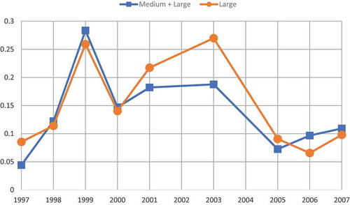
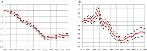
Figures 1 and 2 show the growth of real wages between 1983 and 2012 for the provincial data, and between 1997 and 2007 for the ASIE data, respectively. Both the provincial and ASIE data indicate that real wage growth increased abruptly in the late-1990s, declining towards the middle of the next decade, rebounding somewhat around 2005, and remained substantially higher than in the preceding ten years through at least 2012³. Figures 3 and 4 illustrate the annual growth of labour productivity. Both the provincial and ASIE data suggest a decline in the rate of growth in years following the turn of the millennium. The figures show that labour productivity and real wage growth both accelerated in the late-1990s, a result consistent with induced innovation. In the next section we develop a theoretical model and derive testable hypotheses that will allow for a more rigorous examination of the induced innovation hypothesis.

Figure 1. Provincial data: average real wage growth

Source: Authors’ calculations from China Statistical Yearbooks

Note: Data are provincial averages of wage growth in secondary industry.

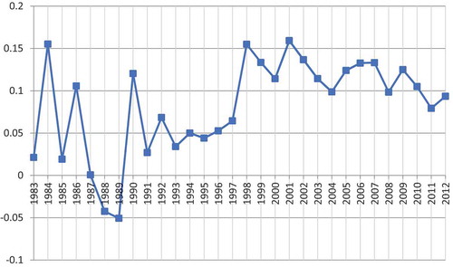
Figure 2. Annual survey of industrial enterprises: real median wage growth

Source: Author calculations from ASIE data. Series show annual proportionate growth of median firm real wages.

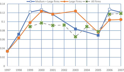
Figure 3. Provincial data: secondary industry labour productivity growth

Source: Authors’ calculations from China Statistical Yearbook

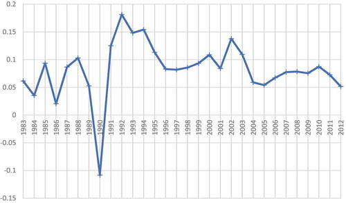
Figure 4. Annual survey of industrial enterprises: median labour productivity growth

Source: Authors’ calculations from ASIE data.

III. Theoretical model and empirical results

Our theoretical model is an adaptation of Acemoglu’s (2010) theoretical framework. Our base model of wage-induced innovation assumes a unitary elasticity of substitution. In Section 4 we relax this rather strict assumption and consider substitution elasticities less than or greater than unity and discuss sensitivity of our basic findings to this more generalized view.

Unitary substitution elasticity benchmark

Following Acemoglu (2010) we specify the production function of the final good producer as follows:

(1) $Y={\alpha }^{-\alpha }(1-\alpha {)}^{-1}(K^{\theta }(AL{)}^{1-\theta }{)}^{\alpha }q(\theta {)}^{1-\alpha }$(1)

where A denotes exogenous labour augmenting technology and ${\alpha }^{-\alpha }(1-\alpha {)}^{-1}$is a convenient normalization used in Acemoglu (2010). The variable $q\left(\theta \right)$ denotes the quantity of an intermediate good embodying technology $\theta$. K and L denote capital and labour, respectively. The objective function of the final good producer is:

(2) $\underset{K,L,q(\theta )}{max}{\alpha }^{-\alpha }(1-\alpha {)}^{-1}{\left(K^{\theta }{(AL)}^{1-\theta }\right)}^{\alpha }q(\theta {)}^{1-\alpha }-W\cdot L-R\cdot K-\chi q(\theta ),$(2)

where W, R and $\chi$ denote wage, rental rate of capital and the price of the intermediate good, respectively. Technology $\theta$ is created and owned by a profit-maximizing monopolist from which the final good producer purchases technology. This setup allows for induced innovation to operate through an endogenous choice of $\theta$ in the final good producer’s maximization problem. As in Acemoglu (2010), we assume K is supplied inelastically at a fixed level$\bar{K}$. Wis exogenously given, which allows us to examine how rising wage rates affect the advancement of induced technological changes.⁴ A positive wage shock not only leads to a standard substitution between capital and labour but may also induce the final good producer to choose a different production process to reduce the impact of rising wages.

As shown in the Online appendix, we define wage-induced innovation as follows:

(3) $\frac{\mathrm{\partial }{\theta }^{\ast }}{\mathrm{\partial }W}>0,$(3)

where ${\theta }^{\ast }$ denotes the optimal choice of technology.⁵ As explained in Wei, Xie, and Zhang (2017), rising wages are an important driver to stimulate China’s growth in innovation. A common empirical approach to examining the price-induced innovation hypothesis focuses on testing the existence of (lagged) price variables in a production or cost function (e.g. Peeters and Surry 2000; Caputo and Paris 2005). Our paper takes a different approach by examining the relationship between labour productivity growth and real wage growth.

Labour productivity growth and real wage growth

In the Online appendix, we derive the relationship between labour productivity and the real wage as follows:

(4) $\frac{Y}{L}=\frac{1}{\alpha (1-\theta )}W.$(4)

Under fixed technology, $\theta$ is constant, implying that labour productivity and the real wage grow at the same rate – a general property of a Cobb-Douglas production function.⁶ However, under induced technological change, $\theta$ increases in response to rising wages, implying that labour productivity grows faster than the real wage. The Online appendix provides a theoretical example of modelling induced technological change.

Define ${\varphi }_t=\left(\frac{1}{\alpha (1-{\theta }_t)}\right)$. Dividing both sides of (4) by W, and taking logs, we characterize the behaviour of over time as:

(4a) $ln\left(\frac{Y_{it}}{L_{it}}\frac{1}{W_{it}}\right)={\varphi }_t+{\eta }_{l(i)}+{\epsilon }_{it}$(4a)

where i denotes province i and ${\eta }_{l(i)}$ captures provincial fixed effects when the provincial data are used; i denotes firm i and ${\eta }_{l(i)}$ captures county fixed effects when we use the ASIE data; ${\varphi }_t$ denotes year fixed effects, and $\frac{1}{e^{{\varphi }_t-{\varphi }_0}}=\frac{1-{\theta }_t}{1-{\theta }_0}$.

Based on equation (4a)(4a) $ln\left(\frac{Y_{it}}{L_{it}}\frac{1}{W_{it}}\right)={\varphi }_t+{\eta }_{l(i)}+{\epsilon }_{it}$(4a) , under induced technological change, rising wage implies that ${\theta }_t$ is greater than ${\theta }_0$: the ratio $\frac{1-{\theta }_t}{1-{\theta }_0}$ should be less than 1.⁷ We estimate equation (4a)(4a) $ln\left(\frac{Y_{it}}{L_{it}}\frac{1}{W_{it}}\right)={\varphi }_t+{\eta }_{l(i)}+{\epsilon }_{it}$(4a) using the ASIE data and report regression results based on the subsample of the Large enterprises in Figure 5, panel A and results for the provincial data covering the years 1978–2011 in panel B. Both sets of results indicate accelerating induced technological change in the late 1990s. After that, both series indicate a weakening of induced technology change, but more so among the set of firms represented in the provincial data.

Figure 5. Estimates of Equation (4a)(4a) $ln\left(\frac{Y_{it}}{L_{it}}\frac{1}{W_{it}}\right)={\varphi }_t+{\eta }_{l(i)}+{\epsilon }_{it}$(4a) based on (1-θ_t)/(1-θ₀) and 95% confidence intervals

Notes: (1) Panel A focuses on the subsample of the Large enterprises; (2) Panel B focuses on provincial data.

Controlling for omitted variables and possible endogeneity

The simple relationship between productivity and wage growth represented in equation (4a)(4a) $ln\left(\frac{Y_{it}}{L_{it}}\frac{1}{W_{it}}\right)={\varphi }_t+{\eta }_{l(i)}+{\epsilon }_{it}$(4a) may yield a biased view of technical change due to omission of variables correlated with both the real wage and the availability of physical capital. To deal with possible omitted variable issues, we take logs of (4) and, adding the year and location identifier (B_it), we obtain the following approximations⁸:

(5) $ln{\left(\frac{Y}{L}\right)}_{it}=B_{it}+\beta ln{W}_{it}+\delta ln{\bar{K}}_{it}+{\epsilon }_{it}.$(5)

Under wage-induced technical change, we expect β > 1. Thus, we test for wage-induced technical change under the following null hypothesis.

Null Hypothesis: β = 1 (in the absence of wage-induced technical change).

Alternative Specification. In an alternative implementation of the induced innovation framework that can aid in testing the robustness of our estimation results, we approach the relationship between labour productivity and the price of labour by substituting the optimal demand for labour into (4) and then taking logs and adding location and year identifiers, to obtain⁹

(6) $ln{\left(\frac{Y}{L}\right)}_{it}=B_{it}+\theta ln{\left(\frac{\bar{K}}{L}\right)}_{it}.$(6)

To examine whether the technology parameter is a function of the real wage we hold constant the influence of the availability of physical capital (allowing for possible capital-induced innovation) and specify:

$\begin{array}{rl}& \theta ={\gamma }_0+{\gamma }_{1}f(W)+{\gamma }_{2}f(\bar{K}),\\ & \mathrm{w}\mathrm{h}\mathrm{e}\mathrm{r}\mathrm{e}f(X)=lnX.\end{array}$

Under wage-induced technical change, we expect ${\gamma }_1>0$. Substituting the preceding specification into (6) we obtain the empirical formulation,^{10 11}:

(7) $ln{\left(\frac{Y}{L}\right)}_{it}=B_{it}+{\gamma }_{0}ln{\left(\frac{\bar{K}}{L}\right)}_{it}+{\gamma }_{1}ln(W_{it})ln{\left(\frac{\bar{K}}{L}\right)}_{it}+{\gamma }_{2}ln({\bar{K}}_{it})ln{\left(\frac{\bar{K}}{L}\right)}_{it}+{\epsilon }_{it}$(7)

Our null hypothesis, indicating the absence of technical change is:

${\gamma }_1=0$

.

Empirical results: Tests with ASIE data

The use of microdata allows us to account for the fact that innovation is more likely among Large firms as suggested in much of the literature on innovation in China (An 2017). Channels that have been proposed in the literature to explain why larger firms tend to invest more in innovation include (i) larger scale that allows larger firms to spread fixed costs of innovation investment over more output (e.g. Schumpeter 1942; Forslid, Okubo, and Ulltveit-Moe 2018); (ii) a broader technological base or a greater ability to absorb riskier innovation investments by pooling risk over a broader portfolio of products (e.g. Nelson 1959). Knott and Vieregger (2020) show that both R&D investment and R&D productivity increase with firm size.

In the ASIE samples, while it seems reasonable to assume that local wage rates are not influenced by individual firm employment decisions, we conduct robustness checks, estimating equations (5)(5) $ln{\left(\frac{Y}{L}\right)}_{it}=B_{it}+\beta ln{W}_{it}+\delta ln{\bar{K}}_{it}+{\epsilon }_{it}.$(5) and (7(7) $ln{\left(\frac{Y}{L}\right)}_{it}=B_{it}+{\gamma }_{0}ln{\left(\frac{\bar{K}}{L}\right)}_{it}+{\gamma }_{1}ln(W_{it})ln{\left(\frac{\bar{K}}{L}\right)}_{it}+{\gamma }_{2}ln({\bar{K}}_{it})ln{\left(\frac{\bar{K}}{L}\right)}_{it}+{\epsilon }_{it}$(7) ) incorporating an instrumental variable (IV) for the local wage as described below. We proceed on the assumption that enterprises’ stock of physical capital are predetermined as discussed above.¹² We include county- and year-fixed effects (FE), as well as region-specific time trends as additional controls (B_it in equations 5 and 7).¹³ We hope inclusion of year FE alleviates concern that our results are driven by drastic SOE reforms in the late 1990s as well as their time-varying impacts across regions. The standard errors are clustered at the county level.

In the IV estimation, the instrumental variable for the firm’s wage is the one-year lagged wage averaged over other counties within the same industry and the same province as the observed firm. Industry categories are (1) Mining; (2) Manufacturing; (3) Production and Distribution of Electricity; and Gas and Water. The identifying assumption of the instrumental variable is that once county-level and year fixed effects are accounted for, the neighbouring counties’ historical economic shocks are not correlated with own county’s contemporaneous economic shocks.

The OLS and IV estimation results for hypotheses on $\beta$ and ${\gamma }_1$ are reported graphically in Figure 6.¹⁴ We see in panel A of Figure 6 that the OLS estimated value of $\beta$ for the two subsamples that exclude the smaller firms generally exceeds 1.0 through the period 1996–2001. This is consistent with our wage-induced innovation hypothesis. However, the estimated value of declines abruptly and remains well below 1.0 between 2001 and 2003, not rising above 1.0 through 2007. Thus, the null of no wage-induced technical change assuming unitary elasticity of substitution is strongly rejected for these two subsamples over the period 1996–2001. The estimated value of for the full sample that includes the smaller-size firms in the ASIE data is consistently less than 1.0 from 1998 through 2007, and its time path follows a roughly similar course to that of the larger-firm subsamples, falling steadily through 2003, rebounding somewhat, but ending in 2007 significantly below its value in 1998. These results indicate that wage induced innovation is weak or absent among smaller-size firms.

Figure 6. Estimates of $\beta$ and ${\gamma }_1$ with $\bar{K}$ in Equations (5) and (7)

Notes: (1) The instrumental variable for the firm’s wage is the one-year lagged average wage over other counties within the same industry and the same province as the observed firm; (2) Dashed lines indicate the 95% confidence intervals.

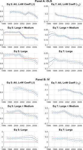
The 2SLS estimate of equation (5)(5) $ln{\left(\frac{Y}{L}\right)}_{it}=B_{it}+\beta ln{W}_{it}+\delta ln{\bar{K}}_{it}+{\epsilon }_{it}.$(5) reported in panel B of Figure 6, with the lagged IV for the industry/county wage as described above, is robust in failing to detect the existence of wage-induced technical change when based on the sample including the smaller-size firms. However, the IV estimated value of for the subsample that includes only large firms significantly exceeds 1.0 through the period 1996–2006, five years beyond evidence consistent with induced innovation revealed in the OLS estimation results for large firms. When the estimation sample is enlarged to include medium firms, the IV estimation results are consistent with the marked decline in the estimated value of $\beta$ in 2001, and not rising above 1.0 through 2007.

As shown in panel A of Figure 6, the OLS estimated value of ${\gamma }_1$ is above zero through the sample period. After 1998, the time paths of ${\gamma }_1$ are closely parallel for all subsamples of the ASIE data, dropping substantially through 2003 until levelling off through 2007 at about three-fourths their value in 1998. Moreover, the time paths for ${\gamma }_1$ are roughly similar to those for equation 5’s $\beta$ shown in panel A, particularly for the Large and Medium and Large firm subsamples. The estimated time paths of the wage coefficients based on both equations (5)(5) $ln{\left(\frac{Y}{L}\right)}_{it}=B_{it}+\beta ln{W}_{it}+\delta ln{\bar{K}}_{it}+{\epsilon }_{it}.$(5) and (7(7) $ln{\left(\frac{Y}{L}\right)}_{it}=B_{it}+{\gamma }_{0}ln{\left(\frac{\bar{K}}{L}\right)}_{it}+{\gamma }_{1}ln(W_{it})ln{\left(\frac{\bar{K}}{L}\right)}_{it}+{\gamma }_{2}ln({\bar{K}}_{it})ln{\left(\frac{\bar{K}}{L}\right)}_{it}+{\epsilon }_{it}$(7) ) indicate a substantial fall-off in the degree of wage innovation over time, with the decline beginning in 2001 in the equation (5)(5) $ln{\left(\frac{Y}{L}\right)}_{it}=B_{it}+\beta ln{W}_{it}+\delta ln{\bar{K}}_{it}+{\epsilon }_{it}.$(5) results and earlier, in 1998, in the equation (7)(7) $ln{\left(\frac{Y}{L}\right)}_{it}=B_{it}+{\gamma }_{0}ln{\left(\frac{\bar{K}}{L}\right)}_{it}+{\gamma }_{1}ln(W_{it})ln{\left(\frac{\bar{K}}{L}\right)}_{it}+{\gamma }_{2}ln({\bar{K}}_{it})ln{\left(\frac{\bar{K}}{L}\right)}_{it}+{\epsilon }_{it}$(7) results.

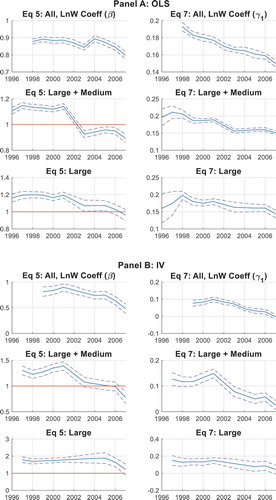
The 2SLS estimates of equation (7)(7) $ln{\left(\frac{Y}{L}\right)}_{it}=B_{it}+{\gamma }_{0}ln{\left(\frac{\bar{K}}{L}\right)}_{it}+{\gamma }_{1}ln(W_{it})ln{\left(\frac{\bar{K}}{L}\right)}_{it}+{\gamma }_{2}ln({\bar{K}}_{it})ln{\left(\frac{\bar{K}}{L}\right)}_{it}+{\epsilon }_{it}$(7) reported in panel B of Figure 6, using the same IV as for estimation of equation (5)(5) $ln{\left(\frac{Y}{L}\right)}_{it}=B_{it}+\beta ln{W}_{it}+\delta ln{\bar{K}}_{it}+{\epsilon }_{it}.$(5) are qualitatively robust to the OLS estimation results in being greater than zero throughout the time period covered in the data. Moreover, there is a very interesting parallel with the estimation results for equation (5)(5) $ln{\left(\frac{Y}{L}\right)}_{it}=B_{it}+\beta ln{W}_{it}+\delta ln{\bar{K}}_{it}+{\epsilon }_{it}.$(5) – OLS and IV estimation results – in indication of a rather pronounced break, with increasingly declining trend following the year 2001. The 2SLS estimation of equation (7)(7) $ln{\left(\frac{Y}{L}\right)}_{it}=B_{it}+{\gamma }_{0}ln{\left(\frac{\bar{K}}{L}\right)}_{it}+{\gamma }_{1}ln(W_{it})ln{\left(\frac{\bar{K}}{L}\right)}_{it}+{\gamma }_{2}ln({\bar{K}}_{it})ln{\left(\frac{\bar{K}}{L}\right)}_{it}+{\epsilon }_{it}$(7) reinforces not only the evidence of falling induced innovation after the year 2001, but also its tendency to disappear in the late sample period.

The inclusion of a measure of physical capital in equations (5)(5) $ln{\left(\frac{Y}{L}\right)}_{it}=B_{it}+\beta ln{W}_{it}+\delta ln{\bar{K}}_{it}+{\epsilon }_{it}.$(5) and (7(7) $ln{\left(\frac{Y}{L}\right)}_{it}=B_{it}+{\gamma }_{0}ln{\left(\frac{\bar{K}}{L}\right)}_{it}+{\gamma }_{1}ln(W_{it})ln{\left(\frac{\bar{K}}{L}\right)}_{it}+{\gamma }_{2}ln({\bar{K}}_{it})ln{\left(\frac{\bar{K}}{L}\right)}_{it}+{\epsilon }_{it}$(7) ) serves to control for omitted variable bias. Estimates of the coefficients $\beta$ and ${\gamma }_1$ are not only very robust to exclusion of the capital-stock variable shown in Figure 7, but we find consistent robustness to 2SLS estimation using an IV for the firm’s wage as described above. Estimates are also robust to the use of a contemporary rather than lagged IV for wage. Details are available from authors on request.

Figure 7. Estimates of $\beta$ and ${\gamma }_1$ without $\bar{K}$ in equations (5) and (7)

Notes: (1) The instrumental variable for the firm’s wage is the one-year lagged average wage over other counties within the same industry and the same province as the observed firm; (2) Dashed lines indicate the 95% confidence intervals.

Empirical results: Tests with provincial data

The provincial data allow us to test the induced innovation hypothesis over the years 1991–2011 compared to 1996–2007 covered by the ASIE data. To control for possible omitted variable bias, we estimate equation (5)(5) $ln{\left(\frac{Y}{L}\right)}_{it}=B_{it}+\beta ln{W}_{it}+\delta ln{\bar{K}}_{it}+{\epsilon }_{it}.$(5) with year and provincial fixed effects as well as region-specific time trends (B_it in equations 5(5) $ln{\left(\frac{Y}{L}\right)}_{it}=B_{it}+\beta ln{W}_{it}+\delta ln{\bar{K}}_{it}+{\epsilon }_{it}.$(5) and 7(7) $ln{\left(\frac{Y}{L}\right)}_{it}=B_{it}+{\gamma }_{0}ln{\left(\frac{\bar{K}}{L}\right)}_{it}+{\gamma }_{1}ln(W_{it})ln{\left(\frac{\bar{K}}{L}\right)}_{it}+{\gamma }_{2}ln({\bar{K}}_{it})ln{\left(\frac{\bar{K}}{L}\right)}_{it}+{\epsilon }_{it}$(7) ). These additional controls capture exogenous shocks to TFP, for example, the differing pace of institutional reforms across different regions in China. Estimation results are reported in Table 3.

Table 3. Estimation results of Equation 5(5) $ln{\left(\frac{Y}{L}\right)}_{it}=B_{it}+\beta ln{W}_{it}+\delta ln{\bar{K}}_{it}+{\epsilon }_{it}.$(5) : provincial secondary industry data

	(1)		(2)
	1st Stage	2nd Stage	1st Stage	2nd Stage
VARIABLES	Log Wage (t-1)	Log Y/L	Log Wage (t-1)	Log Y/L
Log Wage (t-1)		1.648**		1.589***
		(0.653)		(0.609)
Log R&D Stock (t-1)			0.027	−0.043
			(0.064)	(0.182)
Log FDI Stock (t-1)			0.025	0.043
			(0.117)	(0.041)
Log Primary Emp. (t-10)	−0.211**		−0.226***
	(0.011)		(0.081)
Log Secondary K Stock (t-1)			0.064	−0.138
			(0.068)	(0.113)
Observations	604	604	604	604
Years	1991–2011		1991–2011
Test β = 1: p-value	0.321		0.334
Kleibergen-Paap rk Wald F Statistic	6.808		8.240
95% Anderson-Rubin confidence set for β	[0.807, 5.335]		[0.684, 4.181]

Notes:

• Our instrument for Log Wage (t-1) is the (log) ten-year lag of total provincial primary employment.

• Regressions include year and province fixed effects, and region fixed effects interacted with a time trend (current year – 1978).

• Regions: Coast = Fujian, Tianjin, Shandong, Hebei, Beijing, Zhejiang, Hainan, Shanghai, Jiangsu, and Guangdong; Northeast = Jilin, Heilongjiang, and Liaoning; Central = Hubei, Chongqing, Sichuan, Guizhou, Jiangxi, Hunan, Inner Mongolia, Anhui, Guangxi, Yunnan, Henan, and Shanxi; Far West = Gansu, Qinghai, Tibet, Xinjiang, and Ningxia.

• R&D stock are not available for Tibet; FDI stock data are not available for Chongqing or for Tibet in 1992.

• β: see equation (5)(5) $ln{\left(\frac{Y}{L}\right)}_{it}=B_{it}+\beta ln{W}_{it}+\delta ln{\bar{K}}_{it}+{\epsilon }_{it}.$(5) . We used a Stata package, twostepweakiv (Sun 2018), to compute the 95% Anderson-Rubin confidence set for β.

• The standard errors are clustered at the province level. *, **, *** indicate significance levels at 0.1, 0.05, and 0.01, respectively.

To control for the potential problem of endogeneity in the estimation of the wage coefficient with provincial aggregate data, we employ the two-stage least squares (2SLS) method, where the instrumental variable (IV) for provincial real wage is the 10-year lagged size of the provincial primary-industry labour force. Following Lewis, W. Arthur (1954), we assume that China had a large ‘surplus population’ in rural areas before market-oriented reforms that supported worker mobility.¹⁵

The point estimates of approximately 1.6 for the coefficients of the one-year lagged log wage are highly significant in both Models (1) and (2) of Table 3, but the Kleibergen and Paap (2006) rk Wald F statistics for weak identification is only moderately strong.¹⁶ Moreover, the p-value for the test that the estimated coefficient of log real wage is greater than 1.0 is 0.32 in Model (1) and 0.33 in Model (2). The lower bound of the 95% Anderson-Rubin confidence set is below one. Thus, we cannot with a high degree of confidence reject the null hypothesis that the coefficient of log real wage equals 1.0, indicating the absence of wage-induced technical change. The weaker evidence regarding wage-induced innovation may reflect the fact that provincial data include firms of all sizes.

In contrast to a broad literature¹⁷ linking FDI and R&D to innovation, in the presence of the log-wage variable we find no support for a positive link of R&D and/or foreign ownership participation to technology growth (see Model (2) of Table 3).

Estimation results for equation (7)(7) $ln{\left(\frac{Y}{L}\right)}_{it}=B_{it}+{\gamma }_{0}ln{\left(\frac{\bar{K}}{L}\right)}_{it}+{\gamma }_{1}ln(W_{it})ln{\left(\frac{\bar{K}}{L}\right)}_{it}+{\gamma }_{2}ln({\bar{K}}_{it})ln{\left(\frac{\bar{K}}{L}\right)}_{it}+{\epsilon }_{it}$(7) based on provincial aggregates over the period 1991–2011 are reported in Table 4. As in estimation of equation (5)(5) $ln{\left(\frac{Y}{L}\right)}_{it}=B_{it}+\beta ln{W}_{it}+\delta ln{\bar{K}}_{it}+{\epsilon }_{it}.$(5) using the provincial aggregate data, we use 2SLS, where the IV for the provincial real wage is the 10-year lagged size of the provincial primary-industry labour force. The estimate of ${\gamma }_1$ is significantly greater than zero, and its lower bound of the 95% Anderson-Rubin confidence set is above zero regardless of whether the capital-stock variable is included. Thus, this estimation result supports the hypothesis of wage-induced technical change.

Table 4. Estimation results of Equation 7(7) $ln{\left(\frac{Y}{L}\right)}_{it}=B_{it}+{\gamma }_{0}ln{\left(\frac{\bar{K}}{L}\right)}_{it}+{\gamma }_{1}ln(W_{it})ln{\left(\frac{\bar{K}}{L}\right)}_{it}+{\gamma }_{2}ln({\bar{K}}_{it})ln{\left(\frac{\bar{K}}{L}\right)}_{it}+{\epsilon }_{it}$(7) : provincial secondary industry data

	(1)		(2)
	1st Stage	2nd Stage	1st Stage	2nd Stage
VARIABLES	Log Wage (t-1) x Log K/L (t-1)	Log Y/L	Log Wage (t-1) x Log K/L (t-1)	Log Y/L
Log Wage (t-1) x Log K/L (t-1)		0.136***		0.205***
		(0.042)		(0.059)
Log Secondary K Stock (t-1) x Log K/L (t-1)	0.309***	−0.091***
	(0.077)	(0.022)
Log K/L (t-1)	9.086***	−0.059	11.495***	−1.571***
	(0.571)	(0.279)	(0.296)	(0.515)
Log Primary Emp. (t-10) x Log K/L (t-1)	−0.437***		−0.354***
	(0.000)		(0.354)
Observations	642	642	642	642
Years	1991–2011		1991–2011
Kleibergen-Paap rk Wald F Statistic	124.970		61.647
95% Anderson-Rubin confidence set for ${\gamma }_1$	[0.048, 0.216]		[0.094, 0.328]

Notes: The standard errors are clustered at the province level. *, **, *** indicate significance levels at 0.1, 0.05, and 0.01, respectively. ${\gamma }_1$: see equation (7).

The regression results based on both micro (firm-level) and macro (province-level) data indicate that the evidence of wage-induced innovation becomes weaker if we focus on the hypothesis test of instead of ${\gamma }_1$ (which is consistently positive and significant). This is mainly related to the threshold values (depending on the elasticity of substitution between capital and labour) used in our hypothesis tests.

IV. Relaxing the assumption of unitary elasticity of substitution

The unitary elasticity of substitution assumption provides us with a clear analytical benchmark to test wage-induced innovation. To evaluate the sensitivity of our hypothesis tests to the existence of non-unitary substitution elasticity we turn to the CES production function. To help visualize the ambiguity in the impact of induced innovation under the alternative specifications of the substitution elasticity and alternative levels of induced innovation, we perform a simple Monte Carlo simulation experiment.

Theoretical model

We first analyse the firm’s problem under fixed (exogenous) technology, as defined below:

(8) $\underset{K_t{L}_t}{max}{\left(\theta K_t^{\rho }+\left(1-\theta \right){\left(A_t{L}_t\right)}^{\rho }\right)}^{\left(1/\rho \right)}-W_t-R_t\cdot K_t,$(8)

where the parameter A_t denotes labour augmenting technology and the elasticity of substitution between capital and labour is $\frac{1}{1-\rho }$. From the first-order conditions, we solve for the profit-maximizing inputs of L and K and obtain the following result:

(9) $L_t={\theta }^{\frac{1}{\rho }}\frac{K_t}{A_t}{\left({\left(\frac{W_t}{(1-\theta )A_t}\right)}^{\frac{\rho }{1-\rho }}-(1-\theta )\right)}^{\frac{-1}{\rho }}$(9)

From (9) and the CES production function, we derive the output-labour ratio:

(10) $\frac{Y_t}{L_t}={\left(\frac{W_t}{(1-\theta )A_t}\right)}^{\frac{1}{1-\rho }}{A}_t$(10)

Our null hypotheses (absence of induced innovation) on the relationship between labour productivity and wage growth under fixed technology depend critically on the elasticity of substitution. The parameter β is our estimate of the partial derivative of $ln(Y_t/L_t)$ with respect to $ln(W_t)$, and the relationship of our obtained estimate of β to the elasticity of substitution is:

(11) $\hat{\beta }=\frac{\mathrm{\partial }ln(Y_t/L_t)}{\mathrm{\partial }ln(W_t)}=\frac{1}{1-\rho }$(11)

Next, we examine the values of ${\gamma }_1$ implied by the CES production function. Under fixed technology, the capital share parameter, $\theta$, is assumed to be invariant to wage increases.¹⁸ Given the firm’s production function, we can re-write the output-labour ratio:

(12) $\frac{Y_t}{L_t}={\left(\theta {(K_t/L_t)}^{\rho }+(1-\theta )A_t^{\rho }\right)}^{(1/\rho )}$(12)

We focus on the partial derivative of $ln(Y_t/L_t)$ with respect to $ln(K_t/L_t)$ and how it is related to changes in the real wage as reflected in our parameter of interest, ${\gamma }_1$. We define the partial of $ln(Y_t/L_t)$ with respect to $ln(K_t/L_t)$ as ${\xi }_t$ and derive it from equation (12)(12) $\frac{Y_t}{L_t}={\left(\theta {(K_t/L_t)}^{\rho }+(1-\theta )A_t^{\rho }\right)}^{(1/\rho )}$(12) as follows:

(13) ${\xi }_t=\frac{\mathrm{\partial }ln(Y_t/L_t)}{\mathrm{\partial }ln(K_t/L_t)}=\frac{1}{H_t}$(13)

where $H_t=1+\frac{1-\theta }{\theta }(\frac{A_t{L}_t}{K_t}{)}^{\rho }$. We relate ${\gamma }_1$ to the partial derivative of ${\xi }_t$ with respect to $ln(W_t)$, specified as:

(14) $\frac{\mathrm{\partial }{\xi }_t}{\mathrm{\partial }ln(W_t)}=\frac{\rho }{1-\rho }\frac{1}{H_t^2{G}_t^2}(1-\theta {)}^{\frac{1-2\rho }{1-\rho }}(\frac{W_t}{A_t}{)}^{\frac{\rho }{1-\rho }}$(14)

where $G_t={\left(\frac{W_t}{(1-\theta )A_t}\right)}^{\frac{\rho }{1-\rho }}-(1-\theta )$. If we estimate regression models (5) and (7), and assuming that the data are consistent with CES production functions under fixed technology, the predictions of the coefficient estimates based on equations (11)(11) $\hat{\beta }=\frac{\mathrm{\partial }ln(Y_t/L_t)}{\mathrm{\partial }ln(W_t)}=\frac{1}{1-\rho }$(11) and (14(14) $\frac{\mathrm{\partial }{\xi }_t}{\mathrm{\partial }ln(W_t)}=\frac{\rho }{1-\rho }\frac{1}{H_t^2{G}_t^2}(1-\theta {)}^{\frac{1-2\rho }{1-\rho }}(\frac{W_t}{A_t}{)}^{\frac{\rho }{1-\rho }}$(14) ) are:

1. under unitary elasticity of substitution: β = 1 and ${\gamma }_1=0$,

2. for elasticity of substitution < 1: β < 1 and ${\gamma }_1<0$,

3. for elasticity of substitution > 1: β > 1 and ${\gamma }_1>0$.

No single prediction from above is fully consistent with our empirical findings presented in the previous section. Focusing on the ASIE results, we find that β is greater than 1 in the late 1990s but drops below one in the 2000s. We also find that ${\gamma }_1$ is positive with a rising trend in the late 1990s and remains positive but with a declining trend afterwards. If we were to assume that the elasticity of substitution declined from significantly greater than unity to significantly less than unity after 2000 we could ‘explain’ the behaviour of $\beta$ but not the parallel behaviour of ${\gamma }_1$ which remains positive after 2000 instead of becoming negative as would be the case under scenario (ii) above. The assumption with fixed technology is not compatible with our empirical findings regardless of the assumed elasticity of substitution in our CES framework.

If there exists wage induced innovation, our estimate of $\beta$ with respect to $ln(W_t)$ will reflect an additional wage impact beyond what is predicted under fixed technology:

(15) $\hat{\beta }=\frac{\mathrm{\partial }ln(Y_t/L_t)}{\mathrm{\partial }ln(W_t)}=\frac{1}{1-\rho }+\frac{1}{1-\rho }\frac{1}{1-\theta }\frac{\mathrm{\partial }\theta }{\mathrm{\partial }ln(W_t)}>\frac{1}{1-\rho }$(15)

Without specifying a full model, the functional form of $\theta \left(W_t\right)$ is unknown and it is difficult to pin down the threshold value of $\hat{\beta }$ (even for a given value of ρ) to be used in the hypothesis test. However, equation (15)(15) $\hat{\beta }=\frac{\mathrm{\partial }ln(Y_t/L_t)}{\mathrm{\partial }ln(W_t)}=\frac{1}{1-\rho }+\frac{1}{1-\rho }\frac{1}{1-\theta }\frac{\mathrm{\partial }\theta }{\mathrm{\partial }ln(W_t)}>\frac{1}{1-\rho }$(15) indicates that increases with induced innovation compared to the case with fixed technology.

To derive the implications of wage-induced innovation for ${\gamma }_1$, we modify equation (14)(14) $\frac{\mathrm{\partial }{\xi }_t}{\mathrm{\partial }ln(W_t)}=\frac{\rho }{1-\rho }\frac{1}{H_t^2{G}_t^2}(1-\theta {)}^{\frac{1-2\rho }{1-\rho }}(\frac{W_t}{A_t}{)}^{\frac{\rho }{1-\rho }}$(14) to allow for the possibility of a nonmonotonic relationship between wage-induced innovation and the parameter ${\gamma }_1$ as follows:

(16) $\begin{array}{rl}& \frac{\mathrm{\partial }{\xi }_t}{\mathrm{\partial }ln(W_t)}=\frac{{\left(\frac{W_t}{(1-\theta )A_t}\right)}^{\frac{\rho }{1-\rho }}}{H_t^2{G}_t^2}\frac{\mathrm{\partial }\theta }{\mathrm{\partial }ln(W_t)}\\ & \hspace{0.17em}-\frac{\rho }{1-\rho }\frac{1}{H_t^2{G}_t^2}(\frac{W_t}{A_t}{)}^{\frac{\rho }{1-\rho }}(1-\theta {)}^{\frac{-\rho }{1-\rho }}\frac{\mathrm{\partial }\theta }{\mathrm{\partial }ln(W_t)}\\ & \hspace{0.17em}+\frac{\rho }{1-\rho }\frac{1}{H_t^2{G}_t^2}(1-\theta {)}^{\frac{1-2\rho }{1-\rho }}(\frac{W_t}{A_t}{)}^{\frac{\rho }{1-\rho }}\end{array}$(16)

In contrast to the implication in equation (15)(15) $\hat{\beta }=\frac{\mathrm{\partial }ln(Y_t/L_t)}{\mathrm{\partial }ln(W_t)}=\frac{1}{1-\rho }+\frac{1}{1-\rho }\frac{1}{1-\theta }\frac{\mathrm{\partial }\theta }{\mathrm{\partial }ln(W_t)}>\frac{1}{1-\rho }$(15) that wage-induced innovation raises β monotonically, an uncertainty about the relationship arises from the two additional components on the right-hand-side of equation (16)(16) $\begin{array}{rl}& \frac{\mathrm{\partial }{\xi }_t}{\mathrm{\partial }ln(W_t)}=\frac{{\left(\frac{W_t}{(1-\theta )A_t}\right)}^{\frac{\rho }{1-\rho }}}{H_t^2{G}_t^2}\frac{\mathrm{\partial }\theta }{\mathrm{\partial }ln(W_t)}\\ & \hspace{0.17em}-\frac{\rho }{1-\rho }\frac{1}{H_t^2{G}_t^2}(\frac{W_t}{A_t}{)}^{\frac{\rho }{1-\rho }}(1-\theta {)}^{\frac{-\rho }{1-\rho }}\frac{\mathrm{\partial }\theta }{\mathrm{\partial }ln(W_t)}\\ & \hspace{0.17em}+\frac{\rho }{1-\rho }\frac{1}{H_t^2{G}_t^2}(1-\theta {)}^{\frac{1-2\rho }{1-\rho }}(\frac{W_t}{A_t}{)}^{\frac{\rho }{1-\rho }}\end{array}$(16) , the first of which is always positive, leading to a higher value of ${\gamma }_1$ with increasing wage-induced innovation, while the sign of the second component depends on the value of $\rho$. The sign is negative if the substitution elasticity is greater than unity but positive if the substitution elasticity is less than unity.

Under a general CES production function, the regression analysis will become much more complicated, because equations (5)(5) $ln{\left(\frac{Y}{L}\right)}_{it}=B_{it}+\beta ln{W}_{it}+\delta ln{\bar{K}}_{it}+{\epsilon }_{it}.$(5) and (7(7) $ln{\left(\frac{Y}{L}\right)}_{it}=B_{it}+{\gamma }_{0}ln{\left(\frac{\bar{K}}{L}\right)}_{it}+{\gamma }_{1}ln(W_{it})ln{\left(\frac{\bar{K}}{L}\right)}_{it}+{\gamma }_{2}ln({\bar{K}}_{it})ln{\left(\frac{\bar{K}}{L}\right)}_{it}+{\epsilon }_{it}$(7) ) are correctly specified only when the elasticity of substitution is equal to unity. Model misspecifications could also affect the coefficient estimates beyond equations (15)(15) $\hat{\beta }=\frac{\mathrm{\partial }ln(Y_t/L_t)}{\mathrm{\partial }ln(W_t)}=\frac{1}{1-\rho }+\frac{1}{1-\rho }\frac{1}{1-\theta }\frac{\mathrm{\partial }\theta }{\mathrm{\partial }ln(W_t)}>\frac{1}{1-\rho }$(15) and (16(16) $\begin{array}{rl}& \frac{\mathrm{\partial }{\xi }_t}{\mathrm{\partial }ln(W_t)}=\frac{{\left(\frac{W_t}{(1-\theta )A_t}\right)}^{\frac{\rho }{1-\rho }}}{H_t^2{G}_t^2}\frac{\mathrm{\partial }\theta }{\mathrm{\partial }ln(W_t)}\\ & \hspace{0.17em}-\frac{\rho }{1-\rho }\frac{1}{H_t^2{G}_t^2}(\frac{W_t}{A_t}{)}^{\frac{\rho }{1-\rho }}(1-\theta {)}^{\frac{-\rho }{1-\rho }}\frac{\mathrm{\partial }\theta }{\mathrm{\partial }ln(W_t)}\\ & \hspace{0.17em}+\frac{\rho }{1-\rho }\frac{1}{H_t^2{G}_t^2}(1-\theta {)}^{\frac{1-2\rho }{1-\rho }}(\frac{W_t}{A_t}{)}^{\frac{\rho }{1-\rho }}\end{array}$(16) ).

Monte carlo simulation

The data-generating process is described in Table 5. We assume there are 50 regions in each pseudo data set. In each region, wage and the supply of capital stock are exogenously determined, generated from a uniform distribution between 1 and 2. The parameter A_t is considered to represent regular technological progress, widely available to all regions. We normalize A_t to be one.¹⁹ $\theta$ is set to be 0.5 + x$W_t$, where we use x to control the degree of wage-induced innovation.²⁰ Setting x to zero turns off wage-induced innovation. In each data set, we consider three elasticity scenarios: (i) elasticity < 1 ($\rho$ takes a random draw from a uniform distribution between −0.8 and −0.2); (ii) elasticity = 1 (ρ = 0); and (iii) elasticity > 1($\rho$ takes a random draw from a uniform distribution between 0.2 and 0.8). For each elasticity scenario, we generate 1000 pseudo data sets.

Table 5. Monte carlo simulation – parameter values

$W_t$	Uniform (1,2)
$K_t$	Uniform (1,2)
$\rho$	Elasticity of Substitution > 1: Uniform (0.2, 0.8) Elasticity of Substitution < 1: Uniform (−0.8, −0.2) Elasticity of Substitution = 1: 0
$\theta$	0.5 + x$W_t$
$A_t$	1

Simulation results are summarized in Figure 8. The upper panel of Figure 8 presents the boxplots of β estimates, while the lower panel presents the boxplots of ${\gamma }_1$ estimates. Table 6 provides a summary of the predicted signs of β and ${\gamma }_1$ for substitution elasticities less than, equal to, and greater than 1.0 under fixed technology (x = 0) and wage-induced technology (x > 0). We note the following in our empirical results:

1. The combined estimates of β and ${\gamma }_1$ reported in Figures 6 and 7 before 2002 are consistent with induced technology if the substitution elasticity is equal to or less than 1.0 and with fixed technology if the substitution elasticity exceeds 1.0. (We note that the confidence interval for ${\gamma }_1$ is broad enough not to preclude a roughly constant time path for ${\gamma }_1$ > 0 prior to 2002.)

2. Following the year 2001, the behaviour of β is still consistent with induced technology for the elasticity of substitution that is less than 1.0. Although the ${\gamma }_1$ estimates remain positive after 2001, they tend to decline, particularly after 2005, suggestive of a decline in the degree of wage-induced technology.

Table 6. Predictions of $\beta$ and ${\gamma }_1$

Assumed Elasticity of Substitution	Elasticity < 1		Elasticity = 1		Elasticity > 1
Parameters	$\beta$	${\gamma }_1$	$\beta$	${\gamma }_1$	$\beta$	${\gamma }_1$
Fixed Technology (x = 0)	< 1	< 0	1	0	> 1	> 0
Induced Technology (x > 0)	$\frac{\mathrm{\partial }\beta }{\mathrm{\partial }x}>0$, starting from $\beta$ < 1	$\frac{\mathrm{\partial }{y}_1}{\mathrm{\partial }x}>0$, starting from ${\gamma }_1$< 0	$\frac{\mathrm{\partial }\beta }{\mathrm{\partial }x}>0$, starting from $\beta$ = 1	$\frac{\mathrm{\partial }{y}_1}{\mathrm{\partial }x}>0$, starting from ${\gamma }_1$= 0	$\frac{\mathrm{\partial }\beta }{\mathrm{\partial }x}>0$, starting from $\beta$ > 1	$\frac{\mathrm{\partial }{y}_1}{\mathrm{\partial }x}\frac{<}{>}0$, starting from ${\gamma }_1$ > 0

Figure 8. Monte carlo simulation results

Note: In each boxplot, the median is indicated by the central mark; the 25th and 75th percentiles are indicated by the bottom and top edges of the box, respectively; the outliers are marked by the ‘+’ symbol.

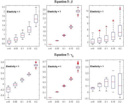
It is also instructive to compare the changes in our estimated β and ${\gamma }_1$ (see Figure 6) with the theoretical results presented in this section. After 2001, our estimate of β falls below one (for small or medium firms), while our estimate of ${\gamma }_1$ declines but remains positive. The joint behaviour of β and ${\gamma }_1$ is not consistent with the assumption of fixed technology. Under fixed technology, the decline in β after 2001 could be explained by a decline in the substitution elasticity from a value greater than one to a value less than one (which we find implausible). However, this would also imply that ${\gamma }_1$ should be negative at the end of our sample period. In fact, our estimated ${\gamma }_1$ remains positive. Evaluation of our empirical results in comparison with the above scenarios leads us to rule out the possibility that fixed technology prevailed during our entire sample period.

The upshot of this simulation exercise is that our empirical results are fully consistent with gradually declining wage-induced innovation when the elasticity of substitution is less than unity. Previous studies of the elasticity of substitution between labour and capital in China provide evidence supporting our induced innovation hypothesis. For example, Mallick (2012) finds that the elasticity of substitution between capital and labour in China is significantly less than unity. Acemoglu and Restrepo (2019) choose an industry-level elasticity of substitution of 0.8, citing Oberfield and Ravel (2014) estimates for United States industry. In other words, our hypothesis tests based on the assumption of unitary elasticity of substitution use conservative threshold values to test wage-induced innovation, which may lead to under-rejection of the null hypothesis. However, given the declining trends in both β and ${\gamma }_1$ estimates, it is still reasonable to conclude that wage-induced technology change had a stronger influence on productivity growth in China in the late 1990s than in the 2000s.

V. Summary and conclusion

Implementing a model developed in Acemoglu (2010) to test hypotheses relating the rate of labour-saving productivity growth to real wage growth and the availability of physical capital in China’s secondary industry, we find evidence supporting wage-induced (labour-saving) innovation among the largest firms beginning in the mid-1990s but not after 2002 (encompassing China’s entry into the WTO) through 2013, where our data end.²¹ To this extent, technical change is not exogenous, as in Molero-Simarro (2017), Ge and Yang (2014), Bai and Qian (2010) and many others.

It will be important for future research to investigate whether adjustments to the increased competitive environment in the years following WTO entry redirected attention towards general efficiency considerations at least temporarily.

We find the absence of stronger evidence supporting wage-induced innovation following China’s WTO accession surprising on its face, and also in light of evidence that productivity (TFP) growth was boosted by WTO accession (Brandt, Van Biesebroeck, and Zhang 2012; Brandt et al. 2017). However, An (2017) notes that ‘Compared with 2002, the percentage of first world innovation in product and process declined sharply [in 2014] indicating that the level of “Created in China” was literally dropping.’

We test sensitivity of our null hypotheses to an assumed elasticity of substitution between labour and capital in a CES framework, finding labour productivity growth could exceed real wage growth under fixed technology if the elasticity exceeds unity. However, the elasticity of substitution exceeding unity is not consistent with published estimates for China (Bai and Qian 2010; Mallick 2012). Importantly, the assumption of fixed technology is not consistent with the changes in our estimated coefficients over time, strengthening our evidence of wage-induced innovation.

The evidence of substantially reduced wage-induced innovation in the approximately five years following China’s accession to WTO is quite robust to estimation with different subsamples and to alternative specifications of regression models. However, our inferences could be biased if our assumption of unitary elasticity of substitution is false. If the elasticity of substitution between capital and labour is less than unity, a decline in the rate of labour productivity growth below the rate of wage growth could still be consistent with induced innovation. Such an increase in the probability of a Type II error would further strengthen empirical support of wage-induced technology change. Additionally, the empirical patterns we find both in regression analysis and simulated patterns based on a more flexible CES framework support wage-induced innovation influencing productivity growth in China, at least in the decade of the 1990s, but less so or not at all after the middle of the next decade.

The industrial explosion that turned China into the ‘workshop of the world’ (Gao 2012) has contributed to dramatic wage increases. As manufacturers start to look elsewhere in order to maintain international competitiveness, other nations hope investors will be attracted to their low-cost labour, producing a similar employment boom. Such hopes might not be realized if China’s rising wages have induced substantial labour-saving innovation whereby unit costs are even lower under the new technology than those in lower-wage labour markets, implying that the employment impact of expanding output is continually damped by rising productivity (Zhong 2015).

Acknowledgements

Comments from the Editor and an anonymous reviewer are gratefully acknowledged. Prof. Xiaojun Wang gratefully acknowledges financial support from the National Natural Science Foundation of China (grant # 71673079).

Disclosure of potential conflicts of interest

No potential conflict of interest was reported by the author(s).

Notes

¹ This is by far the most comprehensive annual survey of industrial firms conducted by the National Bureau of Statistics of China (NBS). It includes all state-owned enterprises and non-state-owned enterprises with sales over 5 million yuan. The only data base that has a larger sample size is the Economic Census, but that is only conducted once in several years. In 2004 when an Economic Census was conducted, this sample account for about 90% of total sales. This data base is widely used in the literature, including Song, Storesletten, and Zilibotti (2011), Hsieh and Klenow (2009), and Brandt, Van Biesebroeck, and Zhang (2012), to name just a few. They are primarily located in secondary industry and results are quite robust to the exclusion of all enterprises not located in this industrial category. Changes in sample definitions and variables measured limit our ability to use the full-time range of available ASIE surveys.

² We have also examined alternative rates for the two-tail trim: 1%, 2%, 5%, 10% and 15%. Our estimation results are quite robust to the trimming of implausibly extreme values.

³ The impact of accelerating wage growth in China has led to an immense literature that we cannot fully cite here. We note the insights in Yang, Chen, and Monarch (2010) and those in the collection of papers on whether China has passed the Lewis Turning Point in China Economic Review (Arthur 2010).

⁴ The theoretical framework can be easily modified to examine the impact of labour scarcity on induced innovation by assuming labour is supplied inelastically at a fixed level $\bar{L}$, as examined in Acemoglu (2010).

⁵ As explained in the Online appendix, to ensure the existence of wage-induced innovation, the wage level should be less than some threshold value that increases with A. We believe this is a realistic assumption in the sample period targeted in our study because of a relatively abundant supply of rural workers. The resulting technology level, ${\theta }^{\ast }$, should be greater than 0.5. This is consistent with China’s income share data: for the industry sector (that is relevant to our provincial and ASIE data), the labour income share was always less than 0.5 1978–2004 (Bai and Qian 2010 Table 4).

⁶ Exogenous technical changes (A), such as exogenous industrial upgrading, will impact labour productivity and wage rates equally, so their growth rates will remain the same.

⁷ It is not appropriate to use equation (4a)(4a) $ln\left(\frac{Y_{it}}{L_{it}}\frac{1}{W_{it}}\right)={\varphi }_t+{\eta }_{l(i)}+{\epsilon }_{it}$(4a) to identify ${\theta }_0$, so we use $\left(1-{\theta }_t\right)/\left(1-{\theta }_0\right)$ to examine how ${\theta }_t$ changes over time.

⁸ The optimal choice of technology can be affected by level of capital stock (this can be demonstrated using our theoretical model), so we include capital stock and B_it as additional control variables to capture non-wage-induced innovation.

⁹ $\bar{K}$ is assumed predetermined as an accumulation of prior investments as in Ge and Yang (2014) and thus is not endogenous with current W. If there is no wage-induced technical change, then a change in W will impact Y/L only through reducing the amount of labour per unit of $\bar{K}$ along the isoquants of an exogenously given production function.

¹⁰ Our key theoretical results shown in equations 5(5) $ln{\left(\frac{Y}{L}\right)}_{it}=B_{it}+\beta ln{W}_{it}+\delta ln{\bar{K}}_{it}+{\epsilon }_{it}.$(5) and 7(7) $ln{\left(\frac{Y}{L}\right)}_{it}=B_{it}+{\gamma }_{0}ln{\left(\frac{\bar{K}}{L}\right)}_{it}+{\gamma }_{1}ln(W_{it})ln{\left(\frac{\bar{K}}{L}\right)}_{it}+{\gamma }_{2}ln({\bar{K}}_{it})ln{\left(\frac{\bar{K}}{L}\right)}_{it}+{\epsilon }_{it}$(7) are conditioned on capital stock. However, the functional form of the conditioning is unknown because the cost function to produce technology $\theta$ can be specified in many different ways. We use a simple log linear function of capital stock in the main text, but we also conducted extensive robustness checks using fractional polynomials and splines. Specifically, we estimated the following specifications:

$ln{\left(\frac{Y}{L}\right)}_{it}=B_{it}+{\beta }_{t}ln{W}_{it}+m({\bar{K}}_{it}\mathrm{o}\mathrm{r}ln{\bar{K}}_{it})+{\epsilon }_{it}(5^{\prime })$ and

$ln{\left(\frac{Y}{L}\right)}_{it}=B_{it}+{\alpha }_{t}ln{\left(\frac{\bar{K}}{L}\right)}_{it}+{\gamma }_{t}ln{W}_{it}\cdot ln{\left(\frac{\bar{K}}{L}\right)}_{it}+m({\bar{K}}_{it}\mathrm{o}\mathrm{r}ln{\bar{K}}_{it})\cdot ln{\left(\frac{\bar{K}}{L}\right)}_{it}+{\epsilon }_{it}(7^{\prime }),$

where m(.) is either a fractional polynomial function or a spline function. This allows us to control for a wide variety of trends in capital stock, which is not an essential part of our analysis. Estimates of primary parameters, i.e. α, β, and γ, are very close to those in the baseline specifications. Estimation results are also robust to inclusion of county-specific fixed effects.

¹¹ Again, when the ASIE data are used, we allow ${\gamma }_0$, ${\gamma }_1$ and ${\gamma }_2$to vary by years.

¹² Rising labour cost is closely related to the dynamics of rural-urban migration (Golley and Meng 2011; Knight, Deng, and Li 2011; Wang et al. 2011; Zhang, Yang, and Wang 2011). An individual firm has very limited power to influence rural-urban migration decisions. In the regression models, we include county fixed effects and regional time trends to control for local common factors that could affect both local wage rates and labour productivity.

¹³ The time trend is defined as (current year – 1978), and the regions are defined as ‘coastal,’ ‘northeast,’ ‘west,’ and ‘far west.’ The provinces included in each region are specified in the notes to table 3.

¹⁴ Estimation results in tabular form are available on request. In particular, we pay special attention to biases and size distortions caused by potentially weak instruments, and we adopt the latest econometric tools, robust to heterogeneity, serial correlation, and clustering. Dealing with weak instruments along with heteroskedasticity and serial correlation when multiple endogenous regressors and instruments are involved is still an open econometric question. We used a Stata package, weakiv (Finlay, Magnusson, and Schaffer 2013), to conduct the Anderson-Rubin test: the null hypothesis is rejected at the 1% level in all regression models. The Anderson-Rubin test is a joint test of the structural parameters (all the coefficients of endogenous regressors are equal to one in equation 5(5) $ln{\left(\frac{Y}{L}\right)}_{it}=B_{it}+\beta ln{W}_{it}+\delta ln{\bar{K}}_{it}+{\epsilon }_{it}.$(5) , or zero in equation 7) and the exogeneity of the instruments.

¹⁵ Estimation results are robust to alternative specifications of the time period for the IV. Since our IV is lagged ten years behind our potentially endogenous independent variable, this approach also limits the years for which we are able to estimate the regression model. We are aware of the pitfalls involved when using lagged values in instrumental variable estimation as noted widely in the literature (e.g. Reed 2015). Nevertheless, we believe these results are of interest as a test of the hypothesis of wage-induced innovation in China, and they add robustness to our results based on individual firms’ data.

¹⁶ In the case with one endogenous regressor and one instrument, the Kleibergen-Paap rk Wald F statistic is equivalent to the Olea, Luis, and Pflueger (2013) effective F statistic.

¹⁷ Much of this literature is summarized in An (2017).

¹⁸ If the elasticity of substitution differs from one, the capital share parameter is not equal to the capital income share in general.

¹⁹ A_t could take a different value in a different time period. The qualitative conclusion of our simulation results is unchanged under different values of A_t.

²⁰ This is a simple shortcut to introduce wage-induced innovation without specifying a full structure of the model to endogenize the choice of technology. We have also explored alternative specifications ($\theta$ = 0.5 + x$\cdot (ln(W_t)+ln(K_t)$) and $\theta$ = 0.5 + x$\cdot ln(W_t)$), and the qualitative conclusion remains unchanged.

²¹ We note that our evidence of the timing of induced innovation is roughly consistent with Li et al. (2012)’s citation of Ceglowski and Golub (2007), that the ratio of Chinese wages to labour productivity declined substantially from the 1980s through the middle of the next decade.

Technical Appendix

Setup:

• A representative firm produces the final good using two factors of production, labour and capital. The price of the final good is normalized to one.

• Technologies are created and supplied by a profit-maximizing monopolist.

• In Acemoglu’s (2010) M economy, the supplies of the productive factors are assumed to be given. We adopt a similar setup, except that the wage (W) instead of the labour supply is given. The goal is to examine how rising wages affect the advancement of induced technological changes. The supply of K is fixed at $\bar{K}$ in the short run.

Final-Good Producer

The objective function of the final-good producer:

$\underset{K,L,q\left(\theta \right)}{max}{\alpha }^{-\alpha }{\left(1-\alpha \right)}^{-1}{\left(K^{\theta }{\left(AL\right)}^{1-\theta }\right)}^{\alpha }q{\left(\theta \right)}^{1-\alpha }-W\cdot L-R\cdot K-\chi q\left(\theta \right)$

$\theta$: technology

$q\left(\theta \right)$: quantity of an intermediate good embodying technology $\theta$

$\chi$: price of the intermediate good

A: labour augmenting technology

${\alpha }^{-\alpha }{\left(1-\alpha \right)}^{-1}$: a convenient normalization used in Acemoglu (2010); $\alpha \in \left(0,1\right)$.

FOCs:

$\left[L\right]:W={\alpha }^{1-\alpha }{\left(1-\alpha \right)}^{-1}\left(1-\theta \right){\left(K^{\theta }{\left(AL\right)}^{1-\theta }\right)}^{\alpha -1}{K}^{\theta }{A}^{1-\theta }{L}^{-\theta }q{\left(\theta \right)}^{1-\alpha }$

$\left[K\right]:R={\alpha }^{1-\alpha }{\left(1-\alpha \right)}^{-1}\theta {\left(K^{\theta }{\left(AL\right)}^{1-\theta }\right)}^{\alpha -1}{K}^{\theta -1}{\left(AL\right)}^{1-\theta }q{\left(\theta \right)}^{1-\alpha }$

$\left[q\left(\theta \right)\right]:{\alpha }^{-\alpha }{\left(1-\alpha \right)}^{-1}\left(1-\alpha \right){\left(K^{\theta }{\left(AL\right)}^{1-\theta }\right)}^{\alpha }q{\left(\theta \right)}^{-\alpha }=\chi$

$q\left(\theta \right)={\alpha }^{-1}{\chi }^{-1/\alpha }\left(K^{\theta }{\left(AL\right)}^{1-\theta }\right)$

$={\alpha }^{1-\alpha }{\left(1-\alpha \right)}^{-1}\left(1-\theta \right){\left(K^{\theta }{\left(AL\right)}^{1-\theta }\right)}^{\alpha -1}$

$W={\alpha }^{1-\alpha }{\left(1-\alpha \right)}^{-1}\left(1-\theta \right){\left(K^{\theta }{\left(AL\right)}^{1-\theta }\right)}^{\alpha -1}{K}^{\theta }{A}^{1-\theta }{L}^{-\theta }q{\left(\theta \right)}^{1-\theta }$

$={\left(1-\alpha \right)}^{-1}\left(1-\theta \right)K^{\theta }{A}^{1-\theta }{L}^{-\theta }{\chi }^{\left(\alpha -1\right)/\alpha }$

$L=K{A}^{\frac{1-\theta }{\theta }}{\left(\frac{1-\theta }{1-\alpha }\frac{1}{W}\right)}^{\frac{1}{\theta }}{\chi }^{\frac{\alpha -1}{\alpha \theta }}$

At the equilibrium, $K=\bar{K}$. Then $L=\bar{K}{A}^{\frac{1-\theta }{\theta }}{\left(\frac{1-\theta }{1-\alpha }\frac{1}{W}\right)}^{\frac{1}{\theta }}{\chi }^{\frac{\alpha -1}{\alpha \theta }}$, and $q\left(\theta \right)={\alpha }^{-1}\bar{K}{\left(\frac{1-\theta }{1-\alpha }\frac{A}{W}\right)}^{\frac{1-\theta }{\theta }}{\chi }^{\frac{\alpha -1-\alpha \theta }{\alpha \theta }}$

The Profit-Maximizing Monopolist

Assumptions:

1. A technology $\theta$ is created at a cost $C\left(\theta \right)$.

$\theta =\frac{1}{1+e^{\varphi }}$

$\varphi =\mathrm{l}\mathrm{n}\left(\frac{1}{\theta }-1\right)$

Assume $C\left(\theta \right)={\left[ln\left(\frac{1}{\theta }-1\right)\right]}^2$.

(2) Once the technology $\theta$ is created, the unit production cost is assumed to be $\frac{1-\alpha }{1-\alpha +\alpha \theta }$ units of the final good. Since the price of the final good is normalized to 1, the unit production cost of the intermediate good is $\frac{1-\alpha }{1-\alpha +\alpha \theta }$.

$\underset{\chi ,\theta }{max}\left(\chi -\frac{1-\alpha }{1-\alpha +\alpha \theta }\right)\cdot {\alpha }^{-1}\bar{K}{\left(\frac{1-\theta }{1-\alpha }\frac{A}{W}\right)}^{\frac{1-\theta }{\theta }}{\chi }^{\frac{\alpha -1-\alpha \theta }{\alpha \theta }}-C\left(\theta \right)$

$\left[\chi \right]:{\chi }^{\frac{\alpha -1-\alpha \theta }{\alpha \theta }}+\left(\chi -\frac{1-\alpha }{1-\alpha +\alpha \theta }\right)\frac{\alpha -1-\alpha \theta }{\alpha \theta }{\chi }^{\frac{\alpha -1-\alpha \theta }{\alpha \theta }-1}=0$

$\chi =1$

Given $\bar{K}$, The problem of the monopolist can be simplified as follows:

$\underset{\theta }{max}\frac{\theta }{1-\alpha +\alpha \theta }\cdot \bar{K}{\left(\frac{1-\theta }{1-\alpha }\frac{A}{W}\right)}^{\frac{1-\theta }{\theta }}-{\left[ln\left(\frac{1}{\theta }-1\right)\right]}^2$

FOC: $\frac{1}{1-\alpha +\alpha \theta }\bar{K}{\left(\frac{1-\theta }{1-\alpha }\frac{A}{W}\right)}^{\left(1-\theta \right)/\theta }\left(\frac{-\alpha \theta }{1-\alpha +\alpha \theta }-\frac{1}{\theta }ln\left(\frac{1-\theta }{1-\alpha }\frac{A}{W}\right)\right)=2\mathrm{l}\mathrm{n}\left(\frac{1}{\theta }-1\right)\frac{1}{{\theta }^2-\theta }$

For the existence of ${\theta }^{\ast }$, we require $\left(1-\alpha \right)\frac{W}{A}$ to be greater than 1:

$\underset{\theta \to 0}{lim}\frac{\theta }{1-\alpha +\alpha \theta }\bar{K}{\left(\frac{1-\theta }{1-\alpha }\frac{A}{W}\right)}^{\frac{1-\theta }{\theta }}=0<\underset{\theta \to 0}{lim}{\left[ln\left(\frac{1}{\theta }-1\right)\right]}^2$

$\underset{\theta \to 1}{lim}\frac{\theta }{1-\alpha +\alpha \theta }\bar{K}{\left(\frac{1-\theta }{1-\alpha }\frac{A}{W}\right)}^{\left(1-\theta \right)/\theta }=\bar{K}<\underset{\theta \to 1}{lim}{\left[ln\left(\frac{1}{\theta }-1\right)\right]}^2$

It is easy to show that the LHS of the FOC is positive given $\left(1-\alpha \right)\frac{\hspace{0.17em}}{A}>1$ and its RHS is positive only when $\theta >$ 0.5, so ${\theta }^{\ast }$ must be between 0.5 and 1.

The objective function of the monopolist has strictly increasing differences in ($W$, $\theta$) if and only if $\frac{{\mathrm{\partial }}^2\frac{\theta }{1-\alpha +\alpha \theta }\bar{K}{\left(\frac{1-\theta }{1-\alpha }\frac{A}{W}\right)}^{\left(1-\theta \right)/\theta }}{\mathrm{\partial }W\mathrm{\partial }\theta }>0$.

$\frac{{\mathrm{\partial }}^2\frac{\theta }{1-\alpha +\alpha \theta }\bar{K}{\left(\frac{1-\theta }{1-\alpha }\frac{A}{W}\right)}^{\frac{1-\theta }{\theta }}}{\mathrm{\partial }W\mathrm{\partial }\theta }>0$ requires that $W<\frac{1-\theta }{1-\alpha }A{e}^{\frac{\alpha {\theta }^2}{1-\alpha +\alpha \theta }+\frac{\theta }{1-\theta }}$. It is easy to show that $\frac{1-\theta }{1-\alpha }A{e}^{\frac{\alpha {\theta }^2}{1-\alpha +\alpha \theta }+\frac{\theta }{1-\theta }}$ is strictly increasing in $\theta$. Then, we define $W_{max}$ as $\frac{1-0.5}{1-\alpha }A{e}^{\frac{\alpha \times {0.5}^2}{1-\alpha +\alpha \times 0.5}+\frac{0.5}{1-0.5}}$, which should be larger than $\frac{A}{1-\alpha }$. Please note that $W<W_{max}$ is only a sufficient condition to ensure the objective function of the monopolist has strictly increasing differences in ($W$, $\theta$).

Given that (a) the objective function is continuously differentiable in $\theta$, (b) $\frac{A}{1-\alpha }<W<W_{max}$ (which ensures that the existence of the solution and the objective function of the monopolist has strictly increasing differences in ($W$, $\theta$)), and (c) the solution is strictly between 0.5 and 1, Topkis’s theorem implies that $\frac{\mathrm{\partial }{\theta }^{\ast }}{\mathrm{\partial }W}>0$. In other words, an increase in $W$ can encourage technological advancement, which we define as a wage-induced technical change.

Output ($Y$) Per Worker

$\frac{Y}{L}=\frac{{\alpha }^{-\alpha }{\left(1-\alpha \right)}^{-1}{\left({\bar{K}}^{\theta }{\left(AL\right)}^{1-\theta }\right)}^{\alpha }{\left({\alpha }^{-1}\left({\bar{K}}^{\theta }{\left(AL\right)}^{1-\theta }\right)\right)}^{1-\alpha }}{L}$

$={\alpha }^{-1}{\left(1-\alpha \right)}^{-1}{\left(\frac{\bar{K}}{L}\right)}^{\theta }{A}^{1-\theta }$

$={\alpha }^{-1}{\left(1-\alpha \right)}^{-1}\frac{W\left(1-\alpha \right)}{1-\theta }$

$=\frac{W}{\alpha \left(1-\theta \right)}$

If $\theta$ is fixed, output per worker increases with $W$. An wage-induced technical change ($W\uparrow \Rightarrow \theta \uparrow$) will further increase the output per worker.

Summary of the Model

1. Given $\bar{K}$, ${\theta }^{\ast }$ increases with $W$: an increase in $W$ will encourage technological advancement, which we define as a wage-induced technical change.

2. Under fixed technology, the output per worker will increase with $W$ (holding $\bar{K}$ fixed). Wage-induced technical change will increase output per worker more than what would be expected on the basis of a pure substitution of capital for labour under fixed technology.

References

- Acemoglu, D. 2010. “When Does Labor Scarcity Encourage Innovation?” Journal of Political Economy 118 (6): 1037–1078. doi:https://doi.org/10.1086/658160.
- Acemoglu, D. 2015. “Localised and Biased Technologies: Atkinson and Stiglitz’s New View, Induced Innovations, and Directed Technological Change.” The Economic Journal 125 (583): 443–463. doi:https://doi.org/10.1111/ecoj.12227.
- Acemoglu, D., and D. Autor. 2011. “Skills, Tasks, and Technologies: Implications for Employment and Earnings.” Handbook of Labor Economics 4b, 1044–1171.
- Acemoglu, D., and P. Restrepo. 2019. “Automation and New Tasks: How Technology Displaces and Reinstates Labor.” Journal of Economic Perspectives 33 (2): 3–30. doi:https://doi.org/10.1257/jep.33.2.3.
- An, T., 2017. “Research on Innovation Behavior Evolution of Chinese Manufacturing Enterprises.” Keynote address presented at Chinese Economists Society 2017 Conference in Nanjing. China. Notes kindly provided by author.
- Lewis, W. Arthur 1954. “Economic Development with Unlimited Supplies of Labor.” The Manchester School 22 (2): 139–191. doi:https://doi.org/10.1111/j.1467-9957.1954.tb00021.x.
- Atkinson, A. B., and J. E. Stiglitz. 1969. “A New View of Technological Change.” The Economic Journal 79 (315): 573–578. doi:https://doi.org/10.2307/2230384.
- Bai, C.-E., and Z. Qian. 2010. “The Factor Income Distribution in China: 1978-2007.” China Economic Review 21 (21): 650–670. doi:https://doi.org/10.1016/j.chieco.2010.08.004.
- Brandt, L., J. Van Biesebroeck, L. Wang, and Y. Zhang. 2017. “WTO Accession and Performance of Chinese Manufacturing Firms.” American Economic Review 107 (9): 2784–2820. doi:https://doi.org/10.1257/aer.20121266.
- Brandt, L., J. Van Biesebroeck, and Y. Zhang. 2012. “Creative Accounting or Creative Destruction? Firm-Level Productivity Growth in Chinese Manufacturing.” Journal of Comparative Economics 97: 339–351.
- Caputo, M., and Q. Paris. 2005. “An Atemporal Microeconomic Theory and an Empirical Test of Price-Induced Technical Progress.” Journal of Productivity Analysis 24 (3): 259–281. doi:https://doi.org/10.1007/s11123-005-4934-3.
- Ceglowski, J., and S. Golub. 2007. “Just How Low are China’s Labour Costs?” World Economy 30 (4): 507–617. doi:https://doi.org/10.1111/j.1467-9701.2007.01006.x.
- Chu, A. C., H. Fan, Y. Furukawa, Z. Kou, and L. Xueyue. Forthcoming. “Minimum Wages, Import Status, and Firms’ Innovation: Theory and Evidence from China.” Economic Inquiry.
- Finlay, K., L. Magnusson, and M. Schaffer, 2013. “WEAKIV: Stata Module to Perform Weak-Instrument-Robust Tests and Confidence Intervals for Instrumental-Variable (IV) Estimation of Linear, Probit and Tobit Models. Statistical Software Components S457684.” Boston College Department of Economics. revised 18 October 2016.
- Forslid, R., T. Okubo, and K. Ulltveit-Moe. 2018. “Why are Firms that Export Cleaner? International Trade, Abatement and Environmental Emissions.” Journal of Environmental Economics and Management 91: 166–183. doi:https://doi.org/10.1016/j.jeem.2018.07.006.
- Freeman, R. B. 2010. “Chapter 70, Labor Regulations, Unions, and Social Protection in Developing Countries: Market Distortions or Efficient Institutions? Chapter 70.” Edited by Dani Rodrik and M. R. Rosenzweig.In Handbook of Development Economics. Vol. 5.4657–4702. Amsterdam: Elsevier.
- Gao, Y. 2012. China as the Workshop of the World: An Analysis at the National and Industry Level of China in the International Division of Labor. London: Routledge.
- Ge, S., and D. T. Yang. 2014. “Changes in China’s Wage Structure.” Journal of the European Economic Association 12 (2): 300–336. doi:https://doi.org/10.1111/jeea.12072.
- Golley, J., and X. Meng. 2011. “Has China Run Out of Surplus Labour?” China Economic Review 22 (4): 555–572. doi:https://doi.org/10.1016/j.chieco.2011.07.006.
- Hau, H., Y. Huang, and G. Wang. 2020. “Firm Response to Competitive Shocks: Evidence from China’s Minimum Wage Policy.” Review of Economic Studies 87 (6): 2639–2671. doi:https://doi.org/10.1093/restud/rdz058.
- Hicks, J. R. 1932. The Theory of Wages. 2nd ed. ed. London: Macmillan.
- Hsieh, C.-T., and P. J. Klenow. 2009. “Misallocation and Manufacturing TFP in China and India.” Quarterly Journal of Economics 12 (4): 1403–1448. doi:https://doi.org/10.1162/qjec.2009.124.4.1403.
- Hu, A. G., and G. H. Jefferson. 2009. “A Great Wall of Patents: What Is behind China’s Recent Patent Explosion?” Journal of Development Economics 90 (1): 57–68. doi:https://doi.org/10.1016/j.jdeveco.2008.11.004.
- Kleibergen, F., and R. Paap. 2006. “Generalized Reduced Rank Tests Using the Singular Value Decomposition.” Journal of Econometrics 133 (1): 97–126. doi:https://doi.org/10.1016/j.jeconom.2005.02.011.
- Knight, J., Q. Deng, and S. Li. 2011. “The Puzzle of Migrant Labour Shortage and Rural Labour Surplus in China.” China Economic Review 22 (4): 585–600. doi:https://doi.org/10.1016/j.chieco.2011.01.006.
- Knott, A. M., and C. Vieregger. 2020. “Reconciling the Firm Size and Innovation Puzzle.” Organization Science 31 (2): 477–488. doi:https://doi.org/10.1287/orsc.2019.1310.
- Li, H., L. Li, B. Wu, and Y. Xiaong. 2012. “The End of Cheap Chinese Labor.” Journal of Economic Perspectives 26 (4): 57–74. doi:https://doi.org/10.1257/jep.26.4.57.
- Mallick, D. 2012. “The Role of the Elasticity of Substitution in Economic Growth: A Cross-Country Investigation.” Labour Economics 19 (5): 682–694. doi:https://doi.org/10.1016/j.labeco.2012.04.003.
- Mayneris, F., S. Poncet, and T. Zhang. 2018. “Improving or Disappearing: Firm-level Adjustments to Minimum Wages in China.” Journal of Development Economics 135: 20–42. doi:https://doi.org/10.1016/j.jdeveco.2018.06.010.
- Molero-Simarro, R. 2017. “Inequality in China Revisited. The Effect of Functional Distribution of Income on Urban Top Incomes, the Urban-Rural Gap and the Gini Index, 1978-2015.” China Economic Review 42: 101–117. doi:https://doi.org/10.1016/j.chieco.2016.11.006.
- Nelson, R. R. 1959. “The Simple Economics of Basic Scientific Research.” Journal of Political Economy 67 (3): 297–306. doi:https://doi.org/10.1086/258177.
- Oberfield, E., and D. Ravel, 2014. “Micro Data and Macro Technology.” NBER Working Paper. 20452.
- Olea, M., J. Luis, and C. Pflueger. 2013. “A Robust Test for Weak Instruments.” Journal of Business and Economic Statistics 31 (3): 358–369. doi:https://doi.org/10.1080/00401706.2013.806694.
- Peeters, L., and Y. Surry. 2000. “Incorporating Price-Induced Innovation in a Symmetric Generalised McFadden Cost Function with Several Outputs.” Journal of Productivity Analysis 14 (1): 53–70. doi:https://doi.org/10.1023/A:1007843928635.
- Reed, W. R. 2015. “On the Practice of Lagging Variables to Avoid Simultaneity.” Oxford Bulletin of Economics and Statistics 77 (6): 897–909. doi:https://doi.org/10.1111/obes.12088.
- Santacreu, A. M., and H. Zhu, 2018. “Has China Overtaken the U.S. In Terms of Innovation?” St. Louis Fed On the Economy Blog. 12 March 2018. https://www.stlouisfed.org/on-the-economy/2018/march/china-overtaken-us-terms-innovation
- Schumpeter, J. A. 1942. Capitalism, Socialism and Democracy. New York: Harper & Row.
- Song, Z., K. Storesletten, and F. Zilibotti. 2011. “Growing Like China.” American Economic Review 101 (1): 196–233. doi:https://doi.org/10.1257/aer.101.1.196.
- Sun, L. 2018. “Implementing Valid Two-Step Identification-Robust Confidence Sets for Linear Instrumental-Variables Models.” Stata Journal, StataCorp LP 18 (4): 803–825. doi:https://doi.org/10.1177/1536867X1801800404.
- Wang, X., J. Huang, L. Zhang, and S. Rozelle. 2011. “The Rise of Migration and the Fall of Self-employment in Rural China’s Labor Market.” China Economic Review 22 (4): 573–584. doi:https://doi.org/10.1016/j.chieco.2011.07.005.
- Wei, S.-J., Z. Xie, and X. Zhang. 2017. “From “Made in China” to “Innovated in China”: Necessity, Prospect, and Challenges.” Journal of Economic Perspectives 31 (1): 49–70. doi:https://doi.org/10.1257/jep.31.1.49.
- Wu, Y. 2016. “China’s Capital Stock Series by Region and Sector.” Frontiers of Economics in China 11: 156–172.
- Yang, D. T., V. Chen, and R. Monarch. 2010. “Rising Wages: Has China Lost Its Global Labor Advantage?” Pacific Economic Review 15 (18): 482–504. doi:https://doi.org/10.1111/j.1468-0106.2009.00465.x.
- Zhang, X., J. Yang, and S. Wang. 2011. “China Has Reached the Lewis Turning Point.” China Economic Review 22 (4): 542–554. doi:https://doi.org/10.1016/j.chieco.2011.07.002.
- Zhong, R., 2015. “For Poor Countries, Well-Worn Path to Development Turns Rocky.” Wall Street Journal 24 November 2015. http://www.wsj.com/articles/for-poor-countries-well-worn-path-to-development-turns-rocky-1448374298