Labour productivity growth and convergence in manufacturing: A nonparametric production frontier approach

ABSTRACT

Labour productivity growth in manufacturing is decomposed into technical efficiency change (movement towards or away from the frontier), technological progress (shifts in the production frontier), and capital accumulation (movement along the frontier) using a nonparametric production frontier method. The results suggest that labour productivity growth is primarily driven by capital accumulation and to a lesser extent technological progress, while technical efficiency is deteriorating over the period 1995–2014. We find that technological progress appears to be non-neutral, as the world manufacturing production frontier expands only at higher capital intensities, benefiting highly industrialized nations. We also find evidence of unconditional convergence in labour productivity for the manufacturing sector. Capital accumulation is the main driver of the observed unconditional convergence, whereas technological change is contributing to divergence rather than convergence. The findings suggest that expanding manufacturing activities through capital accumulation is essential for developing countries to catch-up with developed countries.

KEYWORDS:

• Labour productivity
• Manufacturing industry
• unconditional convergence
• technological change
• data envelopment analysis

JEL Codes:

• O14
• O40
• O47
• C14

I. Introduction

Inspired by the seminal works of Solow (1956, 1957), numerous researches have been focusing on understanding the process of economic growth and convergence (e.g. Romer 1986; Baumol, 1986; Lucas 1988; De Long 1988; Hall and Jones 1999; Easterly and Levine 2001). Specifically, the question of whether there is a tendency of poorer countries to catch-up with rich ones has stimulated both theoretical and empirical research in the area of economic growth.¹ The neoclassical growth model predicts that countries with access to identical technologies and have similar savings and population growth rates should converge to a common income. It implies that poorer countries should grow faster than rich countries since they have higher marginal productivity of capital. Therefore, the neoclassical growth theory predicts ‘conditional convergence’ in the sense that countries will converge to a common income level only if they share similar rates of capital accumulation and population growth. In light of this prediction and the observed lack of (unconditional) convergence in income across countries, empirical growth studies have been investigating the relevant factors that can show evidence of conditional convergence as the theory suggests (e.g. Mankiw, Romer, and Weil 1992; Barro and Sala-i-Martin 1992; Sala-i-Martin 1997; Galor 1996).

In contrast to economies as a whole, Rodrik (2013) documents unconditional convergence in labour productivity in manufacturing activities regardless of geography, policies, or other country-specific characteristics. Rodrik argues that convergence in manufacturing does not aggregate up to the economy as a whole because of its small size compared to nonmanufacturing, which he shows does not exhibit convergence. What is special about manufacturing industries is the production of tradable goods that can be integrated into global production networks quickly, which help to facilitate technology transfer and adoption. They also compete with other efficient foreign suppliers, which necessitates upgrading their operations to maintain competitiveness. These features are lacking in traditional agricultural, many nontradable services, and informal economic activities (Rodrik 2013). Indeed, the expansion of manufacturing activities has been a major force in shaping the modern world. It was the industrial revolution that led to the division of the world economy into rich and poor nations, by enabling for the first time sustained productivity growth in Europe and the United States. Furthermore, it was the development of manufacturing industries that allowed some Eastern countries to catch-up with Western nations (Rodrik 2016).

This paper focuses on labour productivity growth and convergence in manufacturing across countries. Unlike Rodrik (2013), this study goes beyond testing for convergence by analysing the underlying forces behind the observed unconditional convergence in manufacturing. It aims to investigate the role played by technological catch-up (movement towards or away from the frontier), technological change (shifts in the production frontier), and capital accumulation (movement along the frontier) in fostering labour productivity growth and convergence in manufacturing. Specifically, it tries to address the following three research questions:

• Do manufacturing activities exhibit unconditional convergence in labour productivity? If so, how much of the convergence that we observe in manufacturing is due to technological catch-up, technological change, or capital accumulation?

• What are the relative contributions of these three components to labour productivity growth in manufacturing?

• How do technologies in manufacturing change over time?

Using a nonparametric production frontier method, labour productivity growth in manufacturing is decomposed into three components attributable to technological catch-up, technological change, and capital accumulation. The manufacturing production frontier for a sample of 49 OECD and non-OECD countries is constructed using linear programming techniques that neither require the specification of the functional form nor impose any particular market structure as in the traditional parametric approaches. In addition, it allows for the presence of inefficiency in the production process and does not require technological change to be neutral.

The results suggest that labour productivity growth in manufacturing is mainly driven by capital accumulation and to a lesser extent technological progress, while technical efficiency is deteriorating over the period 1995–2014. We find that technological change appears to be non-neutral, as the world manufacturing production frontier expands almost only at higher capital intensities, benefiting highly industrialized nations. We reconfirm the finding by Rodrik (2013) that manufacturing exhibits unconditional convergence in labour productivity. We analyse manufacturing convergence in more detail by looking into the contributions of technical efficiency change, technological change, and capital accumulation. We find that unconditional convergence in manufacturing is primarily driven by faster capital accumulation of less industrialized countries. In contrast, technological change contributed to divergence as the technological frontier expansion appears to be benefiting only developed countries. Technical efficiency did not contribute to the observed convergence as there is no statistically significant relationship between efficiency change and the initial level of labour productivity. The findings suggest that expanding manufacturing activities through capital accumulation is essential for developing countries to catch-up with developed countries.

The paper is organized as follows: Section 2 describes the nonparametric frontier method and the convergence analysis used in the study. The description of the data is provided in section 3. Section 4 presents the results and section 5 performs robustness checks. Finally, section 6 concludes.

II. Methodology

The nonparametric production frontier

Inspired by the seminal works of Färe et al. (1994) and Kumar and Russell (2002),² the worldwide manufacturing production frontier is constructed using a nonparametric deterministic frontier method known as Data Envelopment Analysis (DEA), which was pioneered by Farrell (1957).³ The basic idea of DEA is to construct a piece-wise linear frontier that envelops the data and estimate the associated technical efficiency levels (distances from the frontier) using linear programming techniques. The DEA requires no specification of the functional form of production as it derives the production possibilities set using linear combinations of output–inputs observations. The boundary of the production possibilities set represents the frontier.

In this study, the world manufacturing production frontier is represented by constant returns to scale technology producing aggregate manufacturing output (value-added) $Y$ using two aggregate inputs: physical capital stock$K$ and labour input$L$. Let $Y_{it},K_{it},L_{it},t=1,2,\dots ,T$ and$i=1,2,\dots ,N$, represent $T$ observations on these three variables for each of the $N$ countries. The reference CRS technology for the world manufacturing production in period $t$ is defined by:

(1) ${\mathcal{T}}_t=\left\{⟨Y,K,L⟩\in {\mathbb{R}}_{+}^3|Y\le \sum _i{z}_{it}{Y}_{it},K\ge \sum _i{z}_{it}{K}_{it},L\ge \sum _i{z}_{it}{L}_{it},z_{it}\ge 0\mathrm{\forall }i\right\}$(1)

where $z_{it}$ are the intensity variables that help to form the frontier such that it envelops the data with the smallest convex free disposal cone. As in Färe et al. (1994) and Kumar and Russell (2002), the technology defined above allows the implosion of the technological frontier over time. It means that the frontier in each period is constructed using current period observations only while ignoring previously observed input-output combinations. In other words, technologies available in the past are obsolete and can no longer be used in the current period. More recent studies (e.g. Henderson and Russell 2005; Los and Timmer 2005; Timmer and Los 2005; Badunenko, Henderson, and Russell 2013) utilize the ‘sequential production set’ formulation by Diewert (1980) to preclude implosion of the frontier over time, which in turn make past technologies available in subsequent periods. In this case, the non-imploded reference technology can be defined by:

(2) ${\mathcal{T}}_t=\left\{⟨Y,K,L⟩\in {\mathbb{R}}_{+}^3|Y\le \sum _{\tau \le t}\sum _i{z}_{i\tau }{Y}_{i\tau },K\ge \sum _{\tau \le t}\sum _i{z}_{i\tau }{K}_{i\tau },L\ge \sum _{\tau \le t}\sum _i{z}_{i\tau }{L}_{i\tau },z_{it}\ge 0\mathrm{\forall }i\right\}$(2)

The Farrell (1957) output-based efficiency index for country $i$ at time $t$ is defined by

(3) $T{E}_{it}=\mathrm{m}\mathrm{i}\mathrm{n}\left\{\lambda |Y_{it}/\lambda ,K_{it},L_{it}\in {\mathcal{T}}_t\right\}$(3)

The technical efficiency index measures the ratio of actual to potential output given actual input quantities. The index is equal to one if and only if country $i$ lies on the production frontier at time$t$. It is less than one for countries that are not producing their potential output given the resources they use. The higher the distance from the production frontier, the smaller is the efficiency index. It should be noted that the index only measures relative efficiency to those countries producing at the frontier in the sample.

The DEA involves solving $N$ linear programming models, one for each country, to obtain the estimates of the relative technical efficiency indexes in a given period. The Farrell output-based efficiency index for country $i$ at period $t$ can be obtained by solving the following linear programming model:

$\underset{{\theta }_{it},z_{1t},\dots ,z_{it}}{max}{\theta }_{it}$

$subjectto$

${\theta }_{it}{Y}_{it}\le \sum _{\tau \le t}\sum _i{z}_{i\tau }{Y}_{i\tau }$

(4) $K_{it}\ge \sum _{\tau \le t}\sum _i{z}_{i\tau }{K}_{i\tau }$(4)

$L_{it}\ge \sum _{\tau \le t}\sum _i{z}_{i\tau }{L}_{i\tau }$

$z_{it}\ge 0\mathrm{\forall }i$

where ${\theta }_{it}$ is the maximal proportional amount that output $Y_{it}$ can be expanded while remaining technologically feasible, given the technology ${\mathcal{T}}_t$ and input quantities $K_{it}$ and $L_{it}$. It is the reciprocal of the technical efficiency index$T{E}_{it}$.

DEA is a data-driven approach that relax most of the assumptions imposed in the traditional approaches. However, it is a deterministic approach that does not take into account measurement errors and therefore can be sensitive to outliers. Nonetheless, Giraleas, Emrouznejad, and Thanassoulis (2012) compare different approaches to productivity analysis using Monte Carlo simulation and show that DEA performs well even under modest measurement errors. When measurement errors become large, the performance of all approaches deteriorates rapidly including stochastic methods that assume the existence of noise in the data. According to Giraleas, Emrouznejad, and Thanassoulis (2012), DEA outperforms all other methods when there is functional form misspecification. We use DEA in this study and perform robustness checks to test the sensitivity of the results to the existence potential outliers in the data.

Decomposition of labour productivity growth

Following the approach of Kumar and Russell (2002), labour productivity growth can be decomposed into components attributable to technological change (shifts in the world production frontier), technological catch-up (movements towards or away from the frontier), and capital accumulation (movement along the frontier). The constant returns to scale assumption enable us to draw the technology set in the $⟨y,k⟩$ space, where $y=Y/L$ and $k=K/L$ denote manufacturing value-added per worker and capital per worker, respectively. Thus, the potential output per worker can be written as a function of capital per worker$\bar{y}\left(k\right)$. Let b and c denote the base period and current period, respectively, the potential outputs per worker in the two periods can be defined in terms of the values of technical efficiency obtained from Eq. (3)(3) $T{E}_{it}=\mathrm{m}\mathrm{i}\mathrm{n}\left\{\lambda |Y_{it}/\lambda ,K_{it},L_{it}\in {\mathcal{T}}_t\right\}$(3) as ${\bar{y}}_b\left(k_b\right)=y_b/T{E}_b$ and ${\bar{y}}_c\left(k_c\right)=y_c/T{E}_c$, where $y_b$ and $y_c$ are the observed output per worker in the base and current period, respectively. Therefore, the ratio of current- to base-period output per worker can be written as:

(5) $\frac{y_c}{y_b}=\frac{T{E}_c}{T{E}_b}.\frac{{\bar{y}}_c\left(k_c\right)}{{\bar{y}}_b\left(k_b\right)}$(5)

Multiplying the numerator and denominator by${\bar{y}}_b\left(k_c\right)$, the potential output per worker at current-period capital-labour ratio using base-period technology, we obtain:

(6) $\frac{y_c}{y_b}=\frac{T{E}_c}{T{E}_b}.\frac{{\bar{y}}_c\left(k_c\right)}{{\bar{y}}_b\left(k_c\right)}.\frac{{\bar{y}}_b\left(k_c\right)}{{\bar{y}}_b\left(k_b\right)}$(6)

Eq. (6)(6) $\frac{y_c}{y_b}=\frac{T{E}_c}{T{E}_b}.\frac{{\bar{y}}_c\left(k_c\right)}{{\bar{y}}_b\left(k_c\right)}.\frac{{\bar{y}}_b\left(k_c\right)}{{\bar{y}}_b\left(k_b\right)}$(6) decomposes the relative change in labour productivity in the two periods into: 1) efficiency change$\frac{T{E}_c}{T{E}_b}$; 2) Technological change$\frac{{\bar{y}}_c\left(k_c\right)}{{\bar{y}}_b\left(k_c\right)}$; and 3) capital accumulation $\frac{{\bar{y}}_b\left(k_c\right)}{{\bar{y}}_b\left(k_b\right)}$ (i.e. the effect of the change in the capital intensity).

The decomposition in Eq. (6)(6) $\frac{y_c}{y_b}=\frac{T{E}_c}{T{E}_b}.\frac{{\bar{y}}_c\left(k_c\right)}{{\bar{y}}_b\left(k_c\right)}.\frac{{\bar{y}}_b\left(k_c\right)}{{\bar{y}}_b\left(k_b\right)}$(6) calculates technological change $\frac{{\bar{y}}_c\left(k_c\right)}{{\bar{y}}_b\left(k_c\right)}$ by the shift in the frontier in the output direction at the current period capital-labour ratio. It also calculates capital accumulation $\frac{{\bar{y}}_b\left(k_c\right)}{{\bar{y}}_b\left(k_b\right)}$ along the base-period frontier. An alternative decomposition that calculates technological change at the base-period capital-labour ratio and capital accumulation by movements along the current-period frontier can be derived by multiplying the numerator and denominator in Eq. (5)(5) $\frac{y_c}{y_b}=\frac{T{E}_c}{T{E}_b}.\frac{{\bar{y}}_c\left(k_c\right)}{{\bar{y}}_b\left(k_b\right)}$(5) by ${\bar{y}}_c\left(k_b\right)$ instead of${\bar{y}}_b\left(k_c\right)$, which yield the following:

(7) $\frac{y_c}{y_b}=\frac{T{E}_c}{T{E}_b}.\frac{{\bar{y}}_c\left(k_b\right)}{{\bar{y}}_b\left(k_b\right)}.\frac{{\bar{y}}_c\left(k_c\right)}{{\bar{y}}_c\left(k_b\right)}$(7)

Thus, the decomposition is path dependent as Eq. (7)(7) $\frac{y_c}{y_b}=\frac{T{E}_c}{T{E}_b}.\frac{{\bar{y}}_c\left(k_b\right)}{{\bar{y}}_b\left(k_b\right)}.\frac{{\bar{y}}_c\left(k_c\right)}{{\bar{y}}_c\left(k_b\right)}$(7) and Eq. (6)(6) $\frac{y_c}{y_b}=\frac{T{E}_c}{T{E}_b}.\frac{{\bar{y}}_c\left(k_c\right)}{{\bar{y}}_b\left(k_c\right)}.\frac{{\bar{y}}_b\left(k_c\right)}{{\bar{y}}_b\left(k_b\right)}$(6) do not necessarily yield the same results. To resolve this issue, Kumar and Russell (2002) follow the approach of Caves, Christensen, and Diewert (1982) and Färe et al. (1994) by adopting the ‘Fisher ideal’ decomposition, based on geometric averages⁴ of the two measures of the effects of technological change and capital deepening, which can be derived by multiplying the numerator and denominator of Eq. (5)(5) $\frac{y_c}{y_b}=\frac{T{E}_c}{T{E}_b}.\frac{{\bar{y}}_c\left(k_c\right)}{{\bar{y}}_b\left(k_b\right)}$(5) by ${\left({\bar{y}}_b\left(k_c\right){\bar{y}}_c\left(k_b\right)\right)}^{1/2}$:

(8) $\frac{y_c}{y_b}=\frac{T{E}_c}{T{E}_b}.{\left(\frac{{\bar{y}}_c\left(k_c\right)}{{\bar{y}}_b\left(k_c\right)}.\frac{{\bar{y}}_c\left(k_b\right)}{{\bar{y}}_b\left(k_b\right)}\right)}^{1/2}.{\left(\frac{{\bar{y}}_b\left(k_c\right)}{{\bar{y}}_b\left(k_b\right)}.\frac{{\bar{y}}_c\left(k_c\right)}{{\bar{y}}_c\left(k_b\right)}\right)}^{1/2}$(8)

$\equiv EFF\times TECH\times KACC$

Where$EFF,$ $TECH,$ and $KACC$ denote efficiency change, technological change, and capital accumulation, respectively. Total Factor Productivity Growth (TFPG) index can be calculated as the product of technical efficiency and technological change indexes (TFPG = EFF×TECH). We use the teradial STATA package developed by Badunenko and Mozharovskyi (2016) to implement the DEA method.

Convergence analysis

The existence of unconditional (absolute) $\beta$-convergence in manufacturing depends on whether there is a tendency of less industrialized countries to grow faster than industrialized countries. In other words, we say that there is unconditional $\beta$-convergence if the growth rate of output per worker is negatively correlated with the initial level of output per worker. Let ${\hat{y}}_{i,t,T}$ be the annualized growth rate of manufacturing output per worker between the base period $t$ and the end period $T$, and let $\mathrm{l}\mathrm{o}\mathrm{g}\left(y_{i,t}\right)$ be the natural logarithm of manufacturing output per worker for country $i$ at time $t$. Consider the following regression:

(9) ${\hat{y}}_{i,t,t+T}=\alpha +\beta \mathrm{l}\mathrm{o}\mathrm{g}\left(y_{i,t}\right)+{\epsilon }_{i,t}$(9)

if we estimate the coefficients and find $\beta <0$, then we say that labour productivity in manufacturing exhibits unconditional convergence.⁵ We also test for the contribution of the three components of labour productivity growth decomposition described earlier by replacing the dependent variable in Eq. (10)(10) $f\left(y\right)=\frac{1}{nh}\sum _{i=1}^{n}K\left(\frac{y-y_i}{h}\right)$(10) with the annualized growth rate of each component. We say that the component is contributing to convergence (divergence) if its annualized growth rate is negatively (positively) correlated with the initial level of labour productivity.

Another way to investigate the existence of convergence is to look at the entire distribution of labour productivity as suggested by Quah (1993, 1996a, 1996b, 1997). Unlike $\beta$-convergence, which focuses on the first moments of the distribution, examining the entire distribution helps to detect the existence of club or twin-peaks convergence. We look at the distribution by estimating the kernel-smoothed density of labour productivity in a given period. The kernel-smoothed density is defined as

(10) $f\left(y\right)=\frac{1}{nh}\sum _{i=1}^{n}K\left(\frac{y-y_i}{h}\right)$(10)

where $K\left(\right)$ is the so-called kernel function and $h$ is the critical bandwidth. As in Quah (1997), I estimate the kernel-smoothed densities by using a Gaussian kernel with Silverman’s rule of thumb for bandwidth selection.⁶

III. Data

The data for manufacturing value added$Y$, employment$L$, and gross fixed capital formation $I$ are obtained from the United Nations Industrial Development Organization’s (UNIDO) INDISTAT2 database. The advantage of INDISTAT2 is the larger coverage of countries beyond OECD countries. Other sectoral databases, such as EU-KLEMS, have limited coverage of countries other than OECD countries. INDISTAT2 covers 173 countries starting from the year 1963. However, there are a large number of missing data, especially for the employment and gross-fixed capital formation (GFCF) variables. To maximize the coverage of countries and minimize the imputation of missing values, the period 1995–2014 is chosen for the analysis.⁷ Specifically, we exclude any country with five or more consecutive missing values for any of the three variables. We also exclude countries with more than seven missing values that are not necessarily consecutive in order. Consequently, the number of countries is reduced to 53 countries. To fill in the missing values of GFCF variable, we calculate the ratio of manufacturing GFCF to the total economy GFCF in the year preceding the missing value. Then, we multiply the ratio by the current year economy-wide GFCF to give a rough estimation of the missing value. The economy-wide GFCF is obtained from the United Nations National Accounts Database. Almost all employment data are available in the period selected. For few observations that are missing, we equalize current period labour productivity with the preceding/following period or their averages. After excluding extreme outliers, I ended up with 49 countries.⁸

We use the Perpetual Inventory Method (PIM) to construct the capital stock for each country as follows:

(11) $K_t=I_t+\left(1-\delta \right)K_{t-1}$(11)

where $\delta$is the depreciation rate of capital and $I_t$ is the gross-fixed capital formation in period t. We assume a constant depreciation rate of 6% across countries.⁹ We also construct capital stocks using different values of $\delta$ and rerun the DEA analysis. The results are reported in Appendix A.

To use PIM, the initial capital stock has to be estimated for each country. Nehru and Dhareshwar (1993) describe several methods for calculating the initial stock of capital. One method is based on the assumption that the capital–output ratio in the initial period is equal to the capital–output ratio in the current period. However, capital stock is unobservable in both periods. The investment series can be used to estimate the current period capital stock through PIM with zero initial capital stock. Then, the capital–output ratio at the current period is used to estimate the initial capital stock. After that, the PIM is used again to derive the capital stock in each period. We will be using this method first for the baseline analysis.

Another method that is widely used in the literature is proposed by Harberger (1978). It assumes that capital–output ratio is constant at the steady state. Therefore, we can obtain the following from Eq. (11)(11) $K_t=I_t+\left(1-\delta \right)K_{t-1}$(11) equation:

(12) $\frac{K_t-K_{t-1}}{K_{t-1}}=-\delta +\frac{I_t}{K_{t-1}}$(12)

Assuming constant capital–output ratio at the steady state implies that the growth rate of capital is equal to the growth rate of output. Therefore, the above equation can be written as

(13) $K_{t-1}=\frac{I_t}{g+\delta }$(13)

where $g$ is the growth rate of output or capital stock.¹⁰ As described in Caselli (2005), we calculate $g$ as the average of the first twenty years of investment series starting from 1970¹¹ For those countries that have investment data starting after 1970, we construct a counterfactual investment series by projecting back all the way to 1970 using the growth rate of the first 20 years. We then use Eq. (13)(13) $K_{t-1}=\frac{I_t}{g+\delta }$(13) to estimate the initial capital stock in 1970 and apply the PIM method to calculate capital stocks for subsequent periods. We use this method as a robustness test and report the associated results in Appendix B.

The UNIDO’s INDISTAT2 data are reported in nominal terms. We deflate the manufacturing GFCF data by dividing it by the ratio of nominal to real GFCF of the total economy, which is obtained from the UN national account database. For the value added data, we use the US producer price index (PPI) as a common deflator¹² for all countries. It should be noted that the UNIDO’s INDISTAT2 is largely derived from industrial surveys. As Rodrik (2013) and Battisti, Del Gatto, and Parmeter (2018) stated, microenterprises and informal firms are often not covered by such surveys. Therefore, the findings using this database should be viewed as an analysis of the organized, formal parts of manufacturing.

IV. Results

Estimation of the manufacturing production frontier

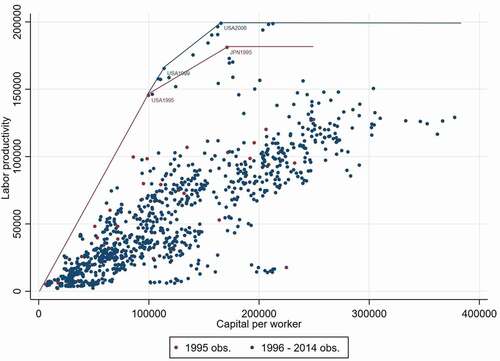
We estimate the manufacturing production frontier and the associated levels of country’s technical efficiency in each period using DEA.¹³ As mentioned in section 3, we adopt intertemporal DEA that precludes implosion of the frontier over time. The assumption of constant returns to scale allows us to draw the frontier in the $\left(y,k\right)$ space as shown in Figure 1. As can be seen, in 1995, the United States and Japan defined the frontier as they both have efficiency scores of one. In fact, the U.S. defines the frontier even at the very low capital intensity levels. These two countries are followed by Germany, which has an efficiency score of 80% in 1995. Countries with middle to high levels of capitalization such as South Korea, Austria, France, and Belgium have efficiency scores of 66%, 57%, 53%, and 70%, respectively. On the other hand, the efficiency scores of countries with low capital labour ratios such as Philippines, Malaysia, and Mexico are 68%, 45%, and 51%, respectively. Table 1 shows technical efficiency indexes of countries in 1995, 2000, 2005, 2010, and 2014. It should be noted that the DEA technical efficiency score estimates are relative to those observations lying on the frontier.

Figure 1. Manufacturing production frontier in 1995.

Table 1. Technical efficiency indexes in 1995, 2000, 2005, 2010, and 2014

Country	1995	2000	2005	2010	2014
Austria	0.57	0.41	0.52	0.52	0.50
Belgium	0.70	0.50	0.62	0.63	0.65
Cyprus	0.37	0.29	0.37	0.29	0.23
Czech Republic	0.29	0.18	0.28	0.26	0.25
Germany	0.80	0.48	0.52	0.49	0.48
Denmark	0.58	0.39	0.48	0.60	0.52
Ecuador	0.20	0.15	0.23	0.30	0.33
Eritrea	0.09	0.07	0.07	0.12	0.14
Spain	0.50	0.37	0.43	0.37	0.37
Estonia	0.57	0.29	0.34	0.28	0.30
Ethiopia	0.37	0.46	0.41	0.38	0.39
Finland	0.61	0.51	0.56	0.49	0.45
France	0.53	0.38	0.43	0.43	0.42
United Kingdom	0.52	0.47	0.51	0.45	0.47
Greece	0.30	0.25	0.38	0.35	0.25
Hong Kong	0.46	0.39	0.26	0.24	0.24
Croatia	0.16	0.13	0.19	0.17	0.15
Hungary	0.15	0.14	0.24	0.22	0.22
India	0.24	0.18	0.25	0.28	0.21
Iran	0.32	0.73	0.30	0.43	0.41
Israel	0.44	0.44	0.35	0.41	0.42
Italy	0.45	0.36	0.41	0.40	0.40
Jordan	0.10	0.11	0.15	0.28	0.34
Japan	1.00	0.86	0.74	0.71	0.57
South Korea	0.66	0.58	0.67	0.53	0.54
Kuwait	0.47	0.32	0.49	0.34	0.36
Latvia	0.34	0.23	0.23	0.17	0.19
Macau	0.37	0.31	0.24	0.13	0.19
Morocco	0.49	0.36	0.37	0.33	0.28
Mexico	0.51	0.56	0.56	0.73	0.75
Malawi	0.13	0.08	0.15	0.20	0.15
Malaysia	0.45	0.33	0.26	0.36	0.42
Netherlands	0.66	0.47	0.59	0.59	0.56
Norway	0.52	0.46	0.59	0.66	0.64
New Zealand	0.47	0.30	0.47	0.44	0.44
Philippines	0.68	0.47	0.28	0.42	0.43
Poland	0.25	0.23	0.34	0.26	0.25
Portugal	0.35	0.21	0.23	0.21	0.19
Romania	0.04	0.04	0.05	0.08	0.08
Singapore	0.68	0.51	0.48	0.54	0.56
Slovak Republic	0.15	0.09	0.17	0.24	0.23
Slovenia	0.40	0.25	0.29	0.25	0.26
Sweden	0.54	0.45	0.52	0.57	0.57
Turkey	0.64	0.49	0.29	0.20	0.18
Uruguay	0.65	0.37	0.28	0.45	0.42
United States	1.00	0.95	1.00	0.86	1.00
Vietnam	0.12	0.14	0.07	0.07	0.09

Figure 2 compares the production frontier in the base year of 1995 with the frontier at the end of the period. As we can see, there is a technological progress driven by the United States at higher capital intensities. In contrast, the frontier has not been shifted at lower levels of capital-labour ratio implying that technological change is non-neutral or factor specific, benefiting more industrialized countries.

Figure 2. Manufacturing production frontiers in 1995 and 2014.

It is well known that the DEA is a biased estimator of the true unobserved frontier as it estimates the frontier only based on observable data. Consequently, the efficiency scores are biased upward as the distance from the true unobserved frontier will always be higher. A remedy to this issue is to perform bootstrapping procedures proposed by Simar and Wilson (1998, 2000, 2002). Table 2 shows biased-corrected efficiency scores and their confidence intervals for the base and end periods of each country in the sample.

Table 2. Bias corrected efficiency indexes and their confidence intervals in 1995 and 2014

	1995				2014
Country	Eff.	Bias corr, Eff.	Lower bound	Upper bound	Eff.	Bias corr, Eff.	Lower bound	Upper bound
Austria	0.57	0.48	0.34	0.56	0.50	0.49	0.46	0.50
Belgium	0.70	0.61	0.43	0.71	0.65	0.64	0.60	0.65
Cyprus	0.37	0.33	0.25	0.37	0.23	0.22	0.21	0.23
Czech Republic	0.29	0.27	0.22	0.30	0.25	0.24	0.23	0.25
Germany	0.80	0.69	0.51	0.79	0.48	0.46	0.43	0.48
Denmark	0.58	0.49	0.36	0.57	0.52	0.50	0.47	0.52
Ecuador	0.20	0.17	0.13	0.20	0.33	0.32	0.30	0.33
Eritrea	0.09	0.09	0.07	0.10	0.14	0.14	0.13	0.14
Spain	0.50	0.42	0.32	0.49	0.37	0.36	0.34	0.37
Estonia	0.57	0.53	0.43	0.59	0.30	0.29	0.28	0.30
Ethiopia	0.37	0.34	0.28	0.38	0.39	0.38	0.37	0.39
Finland	0.61	0.52	0.37	0.61	0.45	0.44	0.42	0.45
France	0.53	0.45	0.32	0.53	0.42	0.41	0.39	0.42
United Kingdom	0.52	0.45	0.33	0.52	0.47	0.45	0.42	0.47
Greece	0.30	0.25	0.18	0.29	0.25	0.24	0.22	0.25
Hong Kong	0.46	0.41	0.31	0.46	0.24	0.23	0.22	0.24
Croatia	0.16	0.14	0.10	0.16	0.15	0.15	0.14	0.15
Hungary	0.15	0.13	0.10	0.15	0.22	0.21	0.19	0.22
India	0.24	0.22	0.18	0.24	0.21	0.21	0.20	0.21
Iran	0.32	0.29	0.23	0.33	0.41	0.40	0.39	0.41
Israel	0.44	0.38	0.29	0.44	0.42	0.40	0.37	0.42
Italy	0.45	0.39	0.29	0.45	0.40	0.39	0.36	0.40
Jordan	0.10	0.08	0.06	0.10	0.34	0.33	0.32	0.34
Japan	1.00	0.84	0.60	0.98	0.57	0.56	0.53	0.57
South Korea	0.66	0.56	0.42	0.65	0.54	0.53	0.50	0.54
Kuwait	0.47	0.40	0.30	0.47	0.36	0.35	0.33	0.36
Latvia	0.34	0.31	0.25	0.35	0.19	0.18	0.18	0.19
Macau	0.37	0.34	0.28	0.38	0.19	0.19	0.18	0.19
Morocco	0.49	0.46	0.37	0.51	0.28	0.27	0.26	0.28
Mexico	0.51	0.46	0.36	0.52	0.75	0.74	0.72	0.75
Malawi	0.13	0.12	0.10	0.13	0.15	0.15	0.14	0.15
Malaysia	0.45	0.41	0.33	0.47	0.42	0.41	0.40	0.42
Netherlands	0.66	0.57	0.40	0.66	0.56	0.55	0.52	0.56
Norway	0.52	0.45	0.32	0.52	0.64	0.63	0.60	0.64
New Zealand	0.47	0.40	0.30	0.47	0.44	0.42	0.40	0.44
Philippines	0.68	0.63	0.51	0.71	0.43	0.43	0.41	0.43
Poland	0.25	0.23	0.19	0.26	0.25	0.24	0.23	0.25
Portugal	0.35	0.31	0.24	0.35	0.19	0.18	0.17	0.19
Romania	0.04	0.04	0.03	0.04	0.08	0.08	0.08	0.08
Singapore	0.68	0.58	0.43	0.67	0.56	0.54	0.51	0.56
Slovak Republic	0.15	0.14	0.11	0.15	0.23	0.22	0.20	0.22
Slovenia	0.40	0.36	0.28	0.41	0.26	0.25	0.24	0.26
Sweden	0.54	0.46	0.33	0.54	0.57	0.56	0.53	0.57
Turkey	0.64	0.57	0.44	0.64	0.18	0.18	0.17	0.18
Uruguay	0.65	0.59	0.46	0.67	0.42	0.41	0.39	0.42
United States	1.00	0.84	0.62	0.98	1.00	0.97	0.92	1.00
Vietnam	0.12	0.11	0.09	0.12	0.09	0.09	0.08	0.09

Labour productivity decomposition and convergence analysis

Table 3 shows the contribution of efficiency change, technological change, and capital accumulation to labour productivity growth from 1995 to 2014. It also shows total factor productivity growth index which is calculated as the product of the first two components. The median growth of labour productivity over the period for the countries covered is 12.7%. This growth is mainly driven by capital accumulation with a median contribution of 30.52%, supported by a minor contribution of technological change of 4.83%. On the other hand, the contribution of efficiency was negative with median efficiency change of −12.15%. The median total factor productivity change was −7.42%, driven by the deterioration of technical efficiency. Since we adopted an intertemporal DEA that preclude implosion of the technological frontier, all countries experienced a non-negative contribution of technological change. Countries with the largest growth in labour productivity include Estonia, Slovak Republic, and Czech Republic. While Slovak Republic labour productivity growth is attributed to both improvement in efficiency and capital accumulation, Estonia and Czech Republic experience deterioration of their efficiency scores which are compensated by the large positive contribution of capital accumulation.

Table 3. Percentage change of labour productivity decomposition indexes, 1995–2014

Country	Labour Productivity change	(EFF – 1) ×100	(TECH – 1) ×100	(KACC – 1) ×100	(TFPG – 1) ×100
Austria	−3.46	−12.15	9.89	0.00	−3.46
Belgium	1.21	−7.90	9.89	0.00	1.21
Croatia	−4.77	−8.11	3.02	0.58	−5.33
Cyprus	1.54	−38.11	4.47	57.04	−35.34
Czech Republic	188.29	−12.57	0.87	226.88	−11.81
Denmark	29.05	−9.94	4.83	36.68	−5.59
Ecuador	22.89	65.15	4.43	−28.74	72.47
Eritrea	16.67	48.42	0.00	−21.39	48.42
Estonia	479.58	−47.82	0.00	1010.76	−47.82
Ethiopia	−26.76	5.66	0.00	−30.68	5.66
Finland	−19.03	−26.32	9.89	−0.00	−19.03
France	−11.73	−19.67	9.89	0.00	−11.73
Germany	−10.72	−39.41	5.05	40.26	−36.35
Greece	−7.47	−17.43	10.69	1.25	−8.60
Hong Kong	−10.02	−47.88	4.88	64.61	−45.34
Hungary	144.62	47.54	4.42	58.78	54.06
India	103.20	−10.69	0.00	127.52	−10.69
Iran	75.14	27.46	0.00	37.41	27.46
Israel	41.39	−5.27	5.32	41.72	−0.23
Italy	8.25	−12.09	9.78	12.17	−3.49
Japan	−37.06	−42.73	9.89	0.00	−37.07
Jordan	92.09	246.46	4.83	−47.11	263.19
Kuwait	−10.02	−23.30	9.94	6.69	−15.68
Latvia	148.00	−43.99	0.00	342.76	−43.99
Macau	28.67	−48.27	0.00	148.73	−48.27
Malawi	16.61	15.68	0.00	0.80	15.68
Malaysia	19.06	−7.42	0.00	28.61	−7.42
Mexico	3.23	46.43	0.00	−29.51	46.43
Morocco	11.33	−43.93	0.00	98.53	−43.93
Netherlands	−6.60	−15.01	9.89	0.00	−6.60
New Zealand	9.21	−7.08	6.10	10.77	−1.41
Norway	36.42	24.14	9.89	0.00	36.42
Philippines	−13.04	−36.93	0.00	37.89	−36.93
Poland	128.37	−2.14	0.00	133.36	−2.14
Portugal	12.70	−44.90	4.78	95.20	−42.27
Romania	159.64	91.05	5.47	28.85	101.50
Singapore	12.40	−18.80	4.83	32.04	−14.88
Slovak Republic	345.52	52.25	1.73	187.66	54.88
Slovenia	38.13	−34.04	4.86	99.70	−30.83
South Korea	1.14	−17.18	9.86	11.16	−9.01
Spain	7.75	−25.71	4.83	38.36	−22.12
Sweden	14.94	4.59	9.89	−0.00	14.93
Turkey	−62.00	−71.03	0.00	31.20	−71.03
United Kingdom	18.32	−10.21	8.27	21.71	−2.78
United States	36.61	−0.16	4.83	30.52	4.66
Uruguay	−8.74	−35.63	0.00	41.79	−35.63
Vietnam	108.01	−23.27	0.00	171.10	−23.27
Median	12.70	−12.15	4.83	30.52	−7.42
OECD	10.96	−12.36	5.19	26.12	−6.10
Non-OECD	16.64	−10.69	0.00	32.04	−10.69

The OECD countries¹⁴ experienced median productivity gains of 10.96% compared to 16.64% for non-OECD countries. The faster productivity growth for non-OECD countries is primarily because of the larger contribution of capital accumulation component. Most non-OECD countries did not benefit from technological change given their low levels of capital intensity. On the other hand, the median contribution of technological change to labour productivity is 5.19% for OECD countries. Indeed, this is the result of the non-neutral technological progress that benefited advanced countries more than developing countries.

For the convergence analysis, we reconfirm the finding by Rodrik (2013) that manufacturing exhibits unconditional convergence in labour productivity. As shown in Table 4, labour productivity growth is negatively correlated with the initial level of labour productivity. We go beyond testing for the unconditional convergence and analyse the contribution of labour productivity growth components to the observed convergence in manufacturing. The results show that convergence in manufacturing is driven by capital accumulation as it is negatively correlated with the initial level of labour productivity. The negative slope is statistically significant as Table 5 shows. Although the technical efficiency change seems to be negatively correlated with the initial level of labour productivity, the negative slope is not statistically significant. Therefore, the technical efficiency index did not contribute to the observed convergence. For technological change, it is in fact positively correlated with the initial levels of labour productivity implying divergence in technology. The positive slope is statistically significant. Figure 3 shows plots of the relationship between labour productivity growth and its three components and the initial level of labour productivity in 1995

Figure 3. Average growth rates of labour productivity and the three decomposition indexes plotted against initial (log) level of labour productivity at the start of the period.

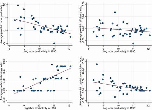
Table 4. Growth regressions of the percentage change in labour productivity and the three decompositions indexes on labour productivity in the base year of 1995

	(1)	(2)	(3)	(4)
	Labour productivity change	(EFF −1) × 100	(TECH −1) × 100	(KACC −1) × 100
Slope	−1.501***	−0.450	0.139***	−1.213**
	(0.364)	(0.269)	(0.016)	(0.483)
Constant	16.938***	4.012	−1.228***	14.434***
	(3.991)	(2.958)	(0.160)	(5.359)
Obs.	47	47	47	47
R-squared	0.380	0.050	0.568	0.207

Robust standard errors are in parenthesis

*** p < 0.01, ** p < 0.05, * p < 0.1

All dependent variables are expressed as annual averages over the sample period (1995–2014)

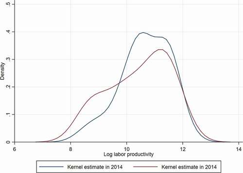
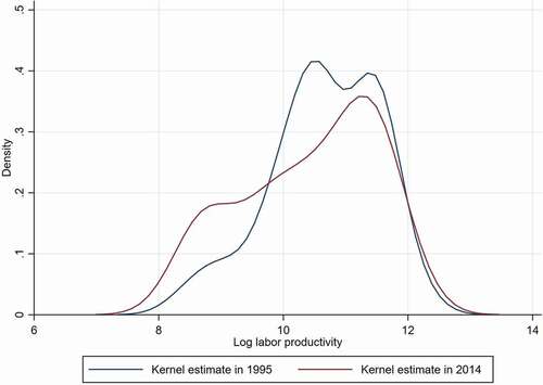
The previous convergence regressions are based on the first moments of the distribution and therefore are susceptible to Quah (1993),Quah (1996a,1997) criticisms of failing to detect the emergence of twin-peaks convergence or bimodality of the distributions. To address this issue, we examine the entire distributions of manufacturing labour productivity in 1995 and 2014 for the countries covered in our sample to see whether such bimodality of distribution exists or not.

Figure 4 shows kernel-smoothed density estimates of manufacturing labour productivity¹⁵ distributions in 1995 and 2014, using Gaussian kernel with Silverman’s rule of thumb¹⁶ for bandwidth selection. In both years, the kernel density estimates appear to be bimodal in shape. However, the distance gap between the two modes has been reduced which can play as an evidence supporting convergence. In other words, the distribution of labour productivity tends to be transforming from bimodal into unimodal distribution as shown in Figure 4.¹⁷

Figure 4. Manufacturing labour productivity distributions in 1995 and 2014.

V. Robustness checks

We assess the robustness of our findings to a number of alternative assumptions for constructing capital stock data as well as the sensitivity of the results to the inclusion of potential outliers’ countries. First, we re-evaluate our analysis using different depreciation rates of capital stock. Appendix A (Tables A1-A6) shows the results using 4% and 8% depreciation rates instead of the baseline assumption of 6%. Technical efficiency estimates and decomposition results appear to be not sensitive to the choice of depreciation rates. We still have capital accumulation as the primary force for labour productivity growth. We notice that the magnitude of the contribution of capital accumulation to labour productivity growth is slightly lower when we use higher depreciation rates and vice versa. Nonetheless, most of the qualitative findings remain the same including the contribution of the decomposition components to labour productivity convergence at 5% significant level.¹⁸

Second, we reconstruct the capital stock series using Harberger (1978) method for the initial capital stock estimates described in section 4. The results are shown in Appendix B (Tables B1-B3). There are no major changes to technical efficiency estimates or to the median contribution labour productivity growth components. We see that the median contribution of capital accumulation is higher whereas median contributions of technological progress and technical efficiency are slightly lower compared to the baseline analysis. For the convergence results, they are similar to the baseline result as Table B3 shows (see Appendix B).

Finally, we examine the sensitivity of the results to the inclusion potential outliers’ countries that can affect the estimation of the DEA frontier (results are in Appendix C, Tables C1-C3). In the baseline analysis, we exclude Ireland and Luxembourg as we believe their value-added data could be inflated by transfer profits. For example, we believe that the Irish data is distorted by the fact that many multinational companies are registered in Ireland for tax purposes while their economic activities might take place elsewhere.¹⁹ Luxembourg’s data also share this feature besides being a small country. The estimated manufacturing production frontier in 1995 does not change by the inclusion of these two countries. However, the frontier in 2014 does change as it massively expands at the very high capital intensities as Figure 5 shows. The large expansion of the technological frontier severely impact technical efficiency estimates for those capital-intensive countries as their distances from the frontier become much larger. Despite this effect, there are no major differences from the baseline results. The median contributions of capital accumulation and technological change components are similar to baseline (31.2% and 5.49% compared to the baseline result 30.52% and 4.83%). Median contribution of technical efficiency index is much lower now (−24.48% compared to −12.15%) driven by the deterioration of OECD countries’ efficiency (non-OECD countries’ efficiency has not changed). The convergence results are similar to the baseline except that we see positive contribution of technical efficiency to convergence (slope is negative and statistically significant at 1%). This is because of the large deterioration of the efficiencies of those countries with high initial level of labour productivity. Thus, the change to the baseline results is that manufacturing convergence in labour productivity is now driven by capital accumulation and technical efficiency compared to capital accumulation alone. In both cases, technological change contributed to divergence, but the magnitude is higher when we include Ireland and Luxembourg (see Table C3 in Appendix C). It is unlikely that such extremely high level of output per worker for Ireland reflects productivity performance. That is why we preferred to exclude these two countries from the baseline analysis.

Figure 5. World production frontier for manufacturing in 1990 and 2014, including Ireland and Luxembourg.

It should be noted that our analysis looks at the manufacturing sector as a whole and does not account for the heterogeneity across manufacturing subsectors. It is possible that the decomposition results differ across manufacturing industries and therefore a separate DEA frontier estimation would be required for each subsector. Due to data limitations, we were unable to perform such analysis. Nonetheless, Rodrik (2013) shows that his unconditional convergence findings still hold, whether using aggregate manufacturing sector or more granular subsectors analysis. Therefore, we believe that our decomposition results at the aggregate level provide insights for the contribution of technical efficiency, technological change, and capital accumulation to labour productivity growth at the granular manufacturing industries.

VI. Conclusion

In this paper, we analyse labour productivity growth and convergence in manufacturing by employing a data-driven frontier approach that relax most of restrictions found in the traditional parametric methods. The method used allows us to decompose labour productivity growth into technological catch-up, technological progress, and capital accumulation, which in turn help us to investigate their contribution to the convergence that we observe in manufacturing.

The decomposition results suggest that labour productivity growth is primarily driven by capital accumulation and to a lesser extent technological progress over the period 1995–2014. Technical efficiency has declined over the two decades studied as manufacturing labour productivity of technological leader countries are growing relatively faster than other countries. This led to widening countries’ distance gaps to the frontier that in turn lower their efficiency levels.

Even though the results show that manufacturing exhibits unconditional convergence in labour productivity, technological change did not contribute to the observed convergence. Indeed, technological progress was rather a force of divergence as it was benefiting industrialized countries with high capital intensities. Nonetheless, larger capital accumulation by less industrialized countries was the main force behind the observed convergence in manufacturing. Looking at the entire distribution of manufacturing labour productivity corroborates the convergence findings. The distribution appears to be transforming from bimodal distribution in 1995 into unimodal distribution in 2014.

The findings shed light on the importance of industrialization to economic growth and convergence. As McMillan and Rodrik (2011) and Rodrik (2013) argue, productivity-enhancing structural change where resources move from low productivity sectors to high productivity sectors is essential for developing countries to catch-up with developed countries. Manufacturing activities are highly productive and exhibit unconditional convergence in labour productivity. Expanding manufacturing activities in developing countries through capital accumulation allows them to access the most productive technologies invented by rich countries, which could help them close the income gap and catch-up with developed countries.

Acknowledgments

I am grateful to Sambit Bhattacharyya, Andy Mckay, Fatih Karanfil, and an anonymous referee for helpful comments and suggestions.

Disclosure statement

No potential conflict of interest was reported by the author(s).

Notes

¹ For surveys of the literature see Sala-i-Martin (1996), Durlauf, Johnson, and Temple (2005), and Badunenko, Henderson, and Zelenyuk (2018).

² The two studies perform DEA for the whole economies. Other studies that use DEA for the analysis of economic growth and convergence include Maudos, Pastor, and Serrano (2000), Gumbau-Albert (2000), Salinas-Jiménez (2003), and Leonida, Petraglia, and Murillo-Zamorano* (2004). For a recent survey, see Badunenko, Henderson, and Zelenyuk (2018).

³ The term DEA was first coined by Charnes, Cooper, and Rhodes (1978)

^{, 4} It should be noted that the geometric mean is more appropriate in this context since we are dealing with growth rates

⁵ See Sala-i-Martin (1996) for a detailed discussion on the classical approach to convergence analysis

⁶ See Silverman (1986) for more details about Silverman’s rule of thumb.

⁷ I still take advantage of the data starting from 1970 to calculate initial capital stock and derive the capital stock for all subsequent periods.

⁸ Four countries are excluded based on some investigation of the investment series and capital stock estimates. The countries are Indonesia, Malta, Sri Lanka and Palestine.

⁹ A constant depreciation rate of 6% is a common assumption in growth accounting studies (e.g. Jones (1997), Hall and Jones (1999), Caselli (2005), Kuralbayeva and Stefanski (2013)).

¹⁰ Studies often define $g$as the growth rate of investment because it is considered a good approximation of capital stock growth rate (e.g. Caselli (2005), Kuralbayeva and Stefanski (2013), Feenstra, Inklaar, and Timmer (2015), Jones (1997))

¹¹ I choose 1970 rather than 1963 because only a small number of countries have data before 1970..

¹² Rodrik (2013) uses a common U.S. dollar inflation rate whereas Battisti, Del Gatto, and Parmeter (2018) perform their analysis using nominal data

¹³ We exclude Ireland and Luxembourg from the baseline analysis and discuss the sensitivity of the results to their inclusion in section 6.

¹⁴ OECD countries: Austria, Belgium, Czech Republic, Denmark, Estonia, Finland, France, Germany, Greece, Hungary, Israel, Italy, Japan, Latvia, Mexico, Netherlands, New Zealand, Norway, Poland, Portugal, Slovak Republic, Slovenia, South Korea, Spain, Sweden, Turkey, United Kingdom, and United States

¹⁵ We use log of labour productivity to avoid estimating the distribution at negative intervals that are not within the domain. In fact, Charpentier and Flachaire (2015) argue that logarithmic transformation of the data is desirable and provide much better fit of the density estimation. Jones (1997b), Birchenall (2001) and Rodrik (2013), among others, use log income values when they show income distribution.

¹⁶ See Silverman (1986) for more details about Silverman’s rule of thumb.

¹⁷ If we choose alternatively Haerdle’s ’better’ Gaussian kernel bandwidth, the distribution in 2014 appears to be unimodal (see Appendix D, Figure D1)

¹⁸ Note that when using the 8% depreciation rate, the contribution of technical efficiency index to convergence become statistically significant at 10%.

¹⁹ See McQuinn et al. (2019) and Rhodes (2018) for more details about the Irish data. Also see the OECD article, Are the Irish 26.3% better off?, October 2016 at http://oecdinsights.org/2016/10/05/are-the-irish-26-3-better-off/

Appendix A:

Results using Different Depreciation Rates

Table A1: Technical efficiency indexes in 1995, 2000, 2005, 2010, 2014 (depreciation rate = 4%)

Country	1995	2000	2005	2010	2014
Austria	0.57	0.41	0.52	0.52	0.50
Belgium	0.70	0.50	0.62	0.63	0.65
Cyprus	0.37	0.28	0.36	0.29	0.22
Czech Republic	0.33	0.21	0.31	0.28	0.27
Germany	0.88	0.53	0.54	0.50	0.49
Denmark	0.57	0.39	0.48	0.60	0.52
Ecuador	0.20	0.15	0.23	0.29	0.31
Eritrea	0.10	0.07	0.07	0.10	0.12
Spain	0.50	0.37	0.44	0.37	0.37
Estonia	0.66	0.35	0.40	0.31	0.33
Ethiopia	0.41	0.48	0.42	0.40	0.43
Finland	0.61	0.51	0.56	0.49	0.45
France	0.53	0.38	0.43	0.43	0.42
United Kingdom	0.51	0.46	0.50	0.45	0.47
Greece	0.29	0.25	0.37	0.35	0.25
Hong Kong	0.42	0.35	0.23	0.22	0.22
Croatia	0.16	0.13	0.18	0.16	0.14
Hungary	0.13	0.13	0.23	0.21	0.21
India	0.27	0.20	0.28	0.31	0.23
Iran	0.33	0.78	0.32	0.45	0.42
Israel	0.47	0.44	0.36	0.42	0.42
Italy	0.45	0.36	0.41	0.40	0.40
Jordan	0.10	0.11	0.14	0.25	0.30
Japan	1.00	0.86	0.74	0.71	0.57
South Korea	0.70	0.58	0.67	0.53	0.54
Kuwait	0.48	0.32	0.49	0.35	0.37
Latvia	0.38	0.26	0.26	0.19	0.20
Macau	0.38	0.31	0.22	0.12	0.16
Morocco	0.55	0.39	0.39	0.36	0.30
Mexico	0.57	0.62	0.60	0.76	0.76
Malawi	0.15	0.09	0.15	0.20	0.15
Malaysia	0.54	0.38	0.29	0.38	0.43
Netherlands	0.66	0.47	0.59	0.59	0.56
Norway	0.52	0.46	0.59	0.66	0.64
New Zealand	0.48	0.30	0.47	0.43	0.43
Philippines	0.73	0.51	0.30	0.43	0.43
Poland	0.25	0.23	0.34	0.26	0.25
Portugal	0.36	0.22	0.23	0.21	0.19
Romania	0.04	0.04	0.05	0.08	0.08
Singapore	0.77	0.52	0.48	0.54	0.56
Slovak Republic	0.17	0.10	0.18	0.26	0.24
Slovenia	0.42	0.26	0.30	0.26	0.26
Sweden	0.54	0.45	0.52	0.57	0.57
Turkey	0.67	0.51	0.31	0.23	0.20
Uruguay	0.70	0.38	0.28	0.45	0.42
United States	1.00	0.95	1.00	0.86	1.00
Vietnam	0.14	0.16	0.09	0.09	0.11

Table A2: Technical efficiency indexes in 1995, 2000, 2005, 2010, 2014 (depreciation rate = 8%)

Country	1995	2000	2005	2010	2014
Austria	0.57	0.41	0.52	0.52	0.50
Belgium	0.70	0.50	0.62	0.63	0.65
Cyprus	0.37	0.30	0.38	0.30	0.24
Czech Republic	0.26	0.17	0.26	0.25	0.25
Germany	0.74	0.46	0.51	0.48	0.48
Denmark	0.58	0.39	0.48	0.60	0.52
Ecuador	0.19	0.15	0.24	0.31	0.34
Eritrea	0.10	0.07	0.07	0.13	0.17
Spain	0.50	0.36	0.42	0.37	0.37
Estonia	0.51	0.26	0.31	0.25	0.28
Ethiopia	0.34	0.46	0.41	0.37	0.35
Finland	0.61	0.51	0.56	0.49	0.45
France	0.53	0.38	0.43	0.43	0.42
United Kingdom	0.53	0.47	0.52	0.45	0.47
Greece	0.31	0.25	0.39	0.36	0.25
Hong Kong	0.49	0.43	0.28	0.26	0.27
Croatia	0.17	0.14	0.20	0.18	0.17
Hungary	0.16	0.15	0.25	0.23	0.22
India	0.22	0.17	0.24	0.26	0.20
Iran	0.32	0.69	0.29	0.42	0.41
Israel	0.43	0.43	0.35	0.41	0.42
Italy	0.45	0.36	0.41	0.40	0.40
Jordan	0.10	0.11	0.17	0.32	0.37
Japan	1.00	0.86	0.74	0.71	0.57
South Korea	0.62	0.58	0.67	0.53	0.54
Kuwait	0.47	0.33	0.49	0.34	0.35
Latvia	0.31	0.21	0.21	0.16	0.18
Macau	0.37	0.32	0.25	0.15	0.23
Morocco	0.46	0.33	0.35	0.31	0.26
Mexico	0.47	0.51	0.54	0.72	0.75
Malawi	0.12	0.08	0.15	0.20	0.16
Malaysia	0.40	0.30	0.25	0.35	0.42
Netherlands	0.66	0.47	0.59	0.59	0.56
Norway	0.52	0.46	0.59	0.66	0.64
New Zealand	0.47	0.30	0.48	0.44	0.45
Philippines	0.65	0.44	0.27	0.42	0.44
Poland	0.26	0.23	0.34	0.26	0.25
Portugal	0.34	0.20	0.22	0.21	0.19
Romania	0.04	0.04	0.05	0.08	0.08
Singapore	0.66	0.50	0.48	0.54	0.56
Slovak Republic	0.13	0.08	0.16	0.23	0.22
Slovenia	0.39	0.25	0.28	0.25	0.26
Sweden	0.54	0.45	0.52	0.57	0.57
Turkey	0.62	0.47	0.27	0.19	0.17
Uruguay	0.62	0.36	0.28	0.44	0.41
United States	1.00	0.95	1.00	0.86	1.00
Vietnam	0.11	0.12	0.06	0.06	0.08

Table A3: Percentage change of labour productivity decomposition indexes, 1995–2014 (depreciation rate = 4%)

Country	Labour Productivity change	(EFF – 1) ×100	(TECH – 1) ×100	(KACC – 1) ×100	(TFPG – 1) ×100
Austria	−3.46	−12.69	10.23	0.30	−3.76
Belgium	1.21	−7.90	9.89	0.00	1.21
Croatia	−4.77	−17.59	5.98	9.04	−12.66
Cyprus	1.54	−39.82	4.92	60.82	−36.86
Czech Republic	188.29	−19.35	0.28	256.47	−19.12
Denmark	29.05	−9.32	4.98	35.57	−4.80
Ecuador	22.89	54.45	4.53	−23.88	61.45
Eritrea	16.67	22.54	0.28	−5.05	22.88
Estonia	479.58	−50.27	0.28	1062.18	−50.13
Ethiopia	−26.76	6.46	0.28	−31.39	6.76
Finland	−19.03	−26.32	9.89	−0.00	−19.03
France	−11.73	−19.67	9.89	0.00	−11.73
Germany	−10.72	−44.52	5.06	53.17	−41.71
Greece	−7.47	−15.80	9.89	−0.00	−7.47
Hong Kong	−10.02	−48.59	4.98	66.72	−46.03
Hungary	144.62	59.10	4.82	46.68	66.77
India	103.20	−12.35	0.28	131.18	−12.10
Iran	75.14	27.16	0.28	37.34	27.52
Israel	41.39	−8.81	5.28	47.27	−4.00
Italy	8.25	−11.54	9.87	11.38	−2.81
Japan	−37.06	−42.73	9.89	0.00	−37.07
Jordan	92.09	207.79	4.98	−40.55	223.12
Kuwait	−10.02	−22.03	9.65	5.24	−14.51
Latvia	148.00	−46.70	0.28	364.00	−46.55
Macau	28.67	−57.40	0.28	201.17	−57.28
Malawi	16.61	−1.05	0.28	17.52	−0.77
Malaysia	19.06	−19.70	0.28	47.86	−19.48
Mexico	3.23	33.44	0.28	−22.86	33.81
Morocco	11.33	−45.61	0.28	104.10	−45.46
Netherlands	−6.60	−15.01	9.89	0.00	−6.60
New Zealand	9.21	−9.47	5.43	14.43	−4.55
Norway	36.42	24.14	9.89	0.00	36.42
Philippines	−13.04	−41.59	0.28	48.48	−41.43
Poland	128.37	1.41	0.28	124.57	1.69
Portugal	12.70	−46.90	5.02	102.11	−44.23
Romania	159.64	88.87	4.98	30.96	98.28
Singapore	12.40	−27.60	4.98	47.88	−23.99
Slovak Republic	345.52	41.95	0.28	212.98	42.35
Slovenia	38.13	−37.34	4.97	110.02	−34.23
South Korea	1.14	−22.04	9.44	18.54	−14.68
Spain	7.75	−25.87	4.98	38.47	−22.18
Sweden	14.94	4.59	9.89	−0.00	14.93
Turkey	−62.00	−69.30	0.28	23.44	−69.21
United Kingdom	18.32	−8.14	9.50	17.63	0.59
United States	36.61	−0.16	4.98	30.34	4.81
Uruguay	−8.74	−39.29	0.28	49.92	−39.12
Vietnam	108.01	−22.66	0.28	168.19	−22.44
Median	12.70	−15.80	4.98	30.96	−11.73
OECD	10.96	−13.85	5.17	20.99	−5.70
Non-OECD	16.61	−19.70	0.28	47.86	−14.51

Table A4: Percentage change of labour productivity decomposition indexes, 1995–2014 (depreciation rate = 8%)

Country	Labour Productivity change	(EFF – 1) ×100	(TECH – 1) ×100	(KACC – 1) ×100	(TFPG – 1) ×100
Austria	−3.46	−12.15	9.89	0.00	−3.46
Belgium	1.21	−7.90	9.89	0.00	1.21
Croatia	−4.77	2.91	0.33	−7.77	3.25
Cyprus	1.54	−36.59	4.02	53.95	−34.04
Czech Republic	188.29	−6.57	1.69	203.43	−4.99
Denmark	29.05	−10.17	4.83	37.03	−5.83
Ecuador	22.89	74.97	4.50	−32.79	82.84
Eritrea	16.67	72.65	0.00	−32.42	72.65
Estonia	479.58	−45.59	0.00	965.25	−45.59
Ethiopia	−26.76	2.27	0.00	−28.39	2.27
Finland	−19.03	−26.32	9.89	−0.00	−19.03
France	−11.73	−19.67	9.89	0.00	−11.73
Germany	−10.72	−35.60	5.20	31.77	−32.25
Greece	−7.47	−19.92	10.61	4.47	−11.42
Hong Kong	−10.02	−43.40	2.49	55.10	−41.99
Hungary	144.62	36.09	4.17	72.55	41.76
India	103.20	−9.32	0.00	124.08	−9.32
Iran	75.14	26.82	0.00	38.10	26.82
Israel	41.39	−2.19	5.54	36.98	3.23
Italy	8.25	−12.56	9.67	12.89	−4.10
Japan	−37.06	−42.73	9.89	0.00	−37.07
Jordan	92.09	283.70	4.83	−52.24	302.23
Kuwait	−10.02	−25.29	10.33	9.16	−17.57
Latvia	148.00	−41.91	0.00	326.93	−41.91
Macau	28.67	−38.80	0.00	110.25	−38.80
Malawi	16.61	34.00	0.00	−12.98	34.00
Malaysia	19.06	5.18	0.00	13.20	5.18
Mexico	3.23	59.10	0.00	−35.12	59.10
Morocco	11.33	−42.83	0.00	94.72	−42.83
Netherlands	−6.60	−15.01	9.89	0.00	−6.60
New Zealand	9.21	−5.09	6.10	8.46	0.70
Norway	36.42	24.14	9.89	0.00	36.42
Philippines	−13.04	−32.42	0.00	28.68	−32.42
Poland	128.37	−6.67	0.00	144.68	−6.67
Portugal	12.70	−42.79	4.61	88.32	−40.15
Romania	159.64	89.98	4.92	30.25	99.33
Singapore	12.40	−15.71	6.94	24.69	−9.86
Slovak Republic	345.52	61.24	2.77	168.86	65.71
Slovenia	38.13	−32.43	4.89	94.88	−29.13
South Korea	1.14	−13.01	10.53	5.19	−3.85
Spain	7.75	−25.55	4.83	38.07	−21.95
Sweden	14.94	4.59	9.89	−0.00	14.93
Turkey	−62.00	−72.30	0.00	37.20	−72.30
United Kingdom	18.32	−11.56	7.44	24.52	−4.98
United States	36.61	−0.16	4.83	30.52	4.66
Uruguay	−8.74	−33.78	0.00	37.83	−33.78
Vietnam	108.01	−24.29	0.00	174.75	−24.29
Median	12.70	−12.15	4.61	28.68	−5.83
OECD	10.96	−12.36	5.37	27.52	−5.41
Non-OECD	16.61	−9.32	0.00	28.68	−9.32

Table A5: Growth regressions of the percentage change in labour productivity and the three decompositions indexes on labour productivity in the base year of 1995 (depreciation rate = 4%)

	(1)	(2)	(3)	(4)
	Labour productivity change	(EFF −1) × 100	(TECH −1) × 100	(KACC −1) × 100
Slope	−1.501***	−0.359	0.138***	−1.306***
	(0.364)	(0.265)	(0.015)	(0.477)
Constant	16.938***	2.864	−1.207***	15.594***
	(3.991)	(2.913)	(0.151)	(5.294)
Obs.	47	47	47	47
R-squared	0.380	0.033	0.579	0.236

Robust standard errors are in parenthesis

*** p < 0.01, ** p < 0.05, * p < 0.1

All dependent variables are expressed as annual averages over the sample period (1995–2014)

Table A6: Growth regressions of the percentage change in labour productivity and the three decomposition indexes on labour productivity in the base year of 1995 (depreciation rate = 8%)

	(1)	(2)	(3)	(4)
	Labour productivity change	(EFF −1) × 100	(TECH −1) × 100	(KACC −1) × 100
Slope	−1.501***	−0.525*	0.141***	−1.138**
	(0.364)	(0.277)	(0.015)	(0.489)
Constant	16.938***	4.944	−1.245***	13.504**
	(3.991)	(3.047)	(0.158)	(5.429)
Obs.	47	47	47	47
R-squared	0.380	0.064	0.565	0.182

Robust standard errors are in parenthesis

*** p < 0.01, ** p < 0.05, * p < 0.1

All dependent variables are expressed as annual averages over the sample period (1995–2014)

Appendix B:

Alternative Estimates of Initial Capital Stocks

Table B1: Technical efficiency indexes in 1995, 2000, 2005, 2010, 2014

Country	1995	2000	2005	2010	2014
Austria	0.57	0.41	0.52	0.52	0.50
Belgium	0.70	0.50	0.62	0.63	0.65
Cyprus	0.36	0.28	0.36	0.28	0.23
Czech Republic	0.17	0.14	0.23	0.23	0.23
Germany	0.64	0.41	0.49	0.46	0.46
Denmark	0.59	0.39	0.48	0.60	0.52
Ecuador	0.19	0.15	0.22	0.28	0.31
Eritrea	0.35	0.14	0.11	0.17	0.20
Spain	0.51	0.37	0.43	0.37	0.37
Estonia	0.63	0.29	0.33	0.26	0.28
Ethiopia	0.47	0.55	0.45	0.39	0.38
Finland	0.61	0.51	0.56	0.49	0.45
France	0.53	0.38	0.43	0.43	0.42
United Kingdom	0.53	0.47	0.51	0.45	0.47
Greece	0.30	0.25	0.38	0.36	0.25
Hong Kong	0.52	0.43	0.27	0.25	0.25
Croatia	0.39	0.24	0.28	0.21	0.19
Hungary	0.15	0.14	0.24	0.22	0.21
India	0.23	0.17	0.24	0.27	0.20
Iran	0.30	0.68	0.28	0.40	0.39
Israel	0.43	0.44	0.35	0.41	0.42
Italy	0.45	0.36	0.41	0.40	0.40
Jordan	0.10	0.10	0.13	0.25	0.30
Japan	1.00	0.86	0.74	0.71	0.57
South Korea	0.64	0.58	0.67	0.53	0.54
Kuwait	0.47	0.32	0.47	0.34	0.36
Latvia	0.95	0.31	0.25	0.17	0.19
Macau	0.38	0.32	0.24	0.13	0.19
Morocco	0.54	0.37	0.36	0.32	0.27
Mexico	0.53	0.55	0.55	0.71	0.72
Malawi	0.12	0.08	0.14	0.19	0.14
Malaysia	0.43	0.31	0.25	0.34	0.40
Netherlands	0.66	0.47	0.59	0.59	0.56
Norway	0.52	0.46	0.59	0.66	0.64
New Zealand	0.47	0.29	0.46	0.43	0.43
Philippines	0.64	0.44	0.26	0.40	0.41
Poland	0.26	0.23	0.33	0.25	0.24
Portugal	0.34	0.20	0.22	0.21	0.19
Romania	0.12	0.08	0.07	0.08	0.08
Singapore	0.67	0.50	0.48	0.54	0.56
Slovak Republic	0.10	0.07	0.14	0.22	0.21
Slovenia	0.46	0.28	0.30	0.25	0.26
Sweden	0.54	0.45	0.52	0.57	0.57
Turkey	0.65	0.49	0.28	0.19	0.18
Uruguay	0.94	0.46	0.32	0.47	0.43
United States	1.00	0.95	1.00	0.86	1.00
Vietnam	0.35	0.18	0.07	0.07	0.09

Table B2: Percentage change of labour productivity decomposition indexes, 1995–2014

Country	Labour Productivity change	(EFF – 1) ×100	(TECH – 1) ×100	(KACC – 1) ×100	(TFPG – 1) ×100
Austria	−3.46	−12.15	9.89	0.00	−3.46
Belgium	1.21	−7.90	9.89	0.00	1.21
Croatia	−4.77	−50.78	0.00	93.46	−50.78
Cyprus	1.54	−37.33	4.24	55.43	−34.67
Czech Republic	188.29	32.12	3.85	110.11	37.21
Denmark	29.05	−11.81	4.83	39.59	−7.55
Ecuador	22.89	59.02	4.25	−25.87	65.78
Eritrea	16.67	−43.15	0.00	105.20	−43.15
Estonia	479.58	−54.89	0.00	1184.94	−54.89
Ethiopia	−26.76	−18.90	0.00	−9.69	−18.90
Finland	−19.03	−26.32	9.89	−0.00	−19.03
France	−11.73	−19.67	9.89	0.00	−11.73
Germany	−10.72	−27.40	9.24	12.56	−20.69
Greece	−7.47	−18.84	10.00	3.64	−10.72
Hong Kong	−10.02	−52.19	4.28	80.46	−50.14
Hungary	144.62	39.01	4.16	68.94	44.79
India	103.20	−12.73	0.00	132.84	−12.73
Iran	75.14	29.36	0.00	35.38	29.36
Israel	41.39	−4.14	4.96	40.53	0.61
Italy	8.25	−12.13	9.35	12.66	−3.91
Japan	−37.06	−42.73	9.89	0.00	−37.07
Jordan	92.09	212.20	4.83	−41.31	227.28
Kuwait	−10.02	−24.13	9.19	8.61	−17.16
Latvia	148.00	−80.22	0.00	1154.08	−80.22
Macau	28.67	−50.79	0.00	161.47	−50.79
Malawi	16.61	14.46	0.00	1.88	14.46
Malaysia	19.06	−7.59	0.00	28.84	−7.59
Mexico	3.23	34.68	0.00	−23.36	34.68
Morocco	11.33	−51.00	0.00	127.19	−51.00
Netherlands	−6.60	−15.01	9.89	0.00	−6.60
New Zealand	9.21	−7.05	6.71	10.10	−0.81
Norway	36.42	24.14	9.89	0.00	36.42
Philippines	−13.04	−36.73	0.00	37.46	−36.73
Poland	128.37	−8.34	0.00	149.14	−8.34
Portugal	12.70	−44.83	4.50	95.49	−42.35
Romania	159.64	−28.54	4.83	246.59	−25.09
Singapore	12.40	−16.49	6.13	26.82	−11.37
Slovak Republic	345.52	110.70	3.91	103.50	118.94
Slovenia	38.13	−43.30	4.47	133.20	−40.77
South Korea	1.14	−15.66	9.58	9.43	−7.58
Spain	7.75	−28.13	4.83	43.02	−24.66
Sweden	14.94	4.59	9.89	−0.00	14.93
Turkey	−62.00	−73.27	0.00	42.19	−73.27
United Kingdom	18.32	−11.87	6.32	26.28	−6.30
United States	36.61	−0.16	4.83	30.52	4.66
Uruguay	−8.74	−54.98	0.00	102.73	−54.98
Vietnam	108.01	−75.44	0.00	746.99	−75.44
Median	12.70	−16.49	4.47	35.38	−11.37
OECD	10.96	−12.14	5.64	19.47	−7.08
Non-OECD	16.64	−28.54	0.00	55.43	−25.09

Table B3: Growth regressions of the percentage change in labour productivity and the three decomposition indexes on labour productivity in the base year of 1995

	(1)	(2)	(3)	(4)
	Labour productivity change	(EFF −1) × 100	(TECH −1) × 100	(KACC −1) × 100
Slope	−1.501***	0.258	0.138***	−1.985***
	(0.364)	(0.385)	(0.015)	(0.544)
Constant	16.938***	−3.971	−1.216***	23.130***
	(3.991)	(4.266)	(0.158)	(6.036)
Obs.	47	47	47	47
R-squared	0.380	0.011	0.567	0.366

Robust standard errors are in parenthesis

*** p < 0.01, ** p < 0.05, * p < 0.1

All dependent variables are expressed as annual averages over the sample period (1995–2014)

Appendix C:

Results Including Ireland and Luxembourg

Table C1: Technical efficiency indexes in 1995, 2000, 2005, 2010, 2014 (Including Ireland and Luxembourg)

Country	1995	2000	2005	2010	2014
Austria	0.57	0.41	0.43	0.42	0.42
Belgium	0.70	0.50	0.48	0.48	0.46
Cyprus	0.37	0.29	0.37	0.29	0.23
Czech Republic	0.29	0.18	0.28	0.26	0.25
Germany	0.80	0.48	0.52	0.48	0.48
Denmark	0.58	0.39	0.45	0.47	0.45
Ecuador	0.20	0.15	0.23	0.30	0.33
Eritrea	0.09	0.07	0.07	0.12	0.14
Spain	0.50	0.37	0.43	0.35	0.32
Estonia	0.57	0.29	0.34	0.28	0.30
Ethiopia	0.37	0.46	0.41	0.38	0.39
Finland	0.61	0.51	0.44	0.38	0.35
France	0.53	0.38	0.38	0.33	0.33
United Kingdom	0.52	0.47	0.50	0.41	0.44
Greece	0.30	0.25	0.38	0.35	0.22
Hong Kong	0.46	0.39	0.25	0.23	0.24
Croatia	0.16	0.13	0.19	0.17	0.15
Hungary	0.15	0.14	0.24	0.22	0.22
India	0.24	0.18	0.25	0.28	0.21
Ireland	0.70	0.94	0.91	1.00	0.88
Iran	0.32	0.73	0.30	0.43	0.41
Israel	0.44	0.44	0.35	0.41	0.41
Italy	0.45	0.36	0.36	0.33	0.32
Jordan	0.10	0.11	0.15	0.28	0.34
Japan	1.00	0.86	0.57	0.55	0.43
South Korea	0.66	0.58	0.51	0.41	0.42
Kuwait	0.47	0.32	0.49	0.34	0.36
Luxembourg	0.66	0.49	0.41	0.36	0.35
Latvia	0.34	0.23	0.23	0.17	0.19
Macau	0.37	0.31	0.24	0.13	0.19
Morocco	0.49	0.36	0.37	0.33	0.28
Mexico	0.51	0.56	0.56	0.73	0.75
Malawi	0.13	0.08	0.15	0.20	0.15
Malaysia	0.45	0.33	0.26	0.36	0.42
Netherlands	0.66	0.47	0.45	0.45	0.42
Norway	0.52	0.46	0.46	0.50	0.48
New Zealand	0.47	0.30	0.47	0.44	0.44
Philippines	0.68	0.47	0.28	0.42	0.43
Poland	0.25	0.23	0.34	0.26	0.25
Portugal	0.35	0.21	0.23	0.21	0.19
Romania	0.04	0.04	0.05	0.06	0.07
Singapore	0.68	0.51	0.38	0.42	0.41
Slovak Republic	0.15	0.09	0.17	0.24	0.23
Slovenia	0.40	0.25	0.29	0.25	0.26
Sweden	0.54	0.45	0.42	0.44	0.43
Turkey	0.64	0.49	0.29	0.20	0.18
Uruguay	0.65	0.37	0.28	0.45	0.42
United States	1.00	0.95	0.98	0.80	0.83
Vietnam	0.12	0.14	0.07	0.07	0.09

Table C2: Percentage change of labour productivity decomposition indexes, 1995–2014 (Including Ireland and Luxembourg)

Country	Labour Productivity change	(EFF – 1) ×100	(TECH – 1) ×100	(KACC – 1) ×100	(TFPG – 1) ×100
Austria	−3.46	−26.77	23.11	7.07	−9.85
Belgium	1.21	−34.01	48.46	3.31	−2.03
Croatia	−4.77	−8.11	3.02	0.58	−5.33
Cyprus	1.54	−38.43	4.74	57.45	−35.51
Czech Republic	188.29	−12.57	0.87	226.88	−11.81
Denmark	29.05	−22.58	13.06	47.42	−12.47
Ecuador	22.89	65.15	4.67	−28.91	72.86
Eritrea	16.67	48.42	0.00	−21.39	48.42
Estonia	479.58	−47.82	0.00	1010.76	−47.82
Ethiopia	−26.76	5.66	0.00	−30.68	5.66
Finland	−19.03	−43.32	33.50	7.00	−24.33
France	−11.73	−37.73	40.76	0.70	−12.35
Germany	−10.72	−40.27	5.80	41.26	−36.81
Greece	−7.47	−26.61	18.73	6.19	−12.86
Hong Kong	−10.02	−48.48	5.49	65.57	−45.65
Hungary	144.62	46.89	4.65	59.13	53.72
India	103.20	−10.69	0.00	127.52	−10.69
Iran	75.14	27.46	0.00	37.41	27.46
Ireland	100.51	26.04	31.90	20.61	66.25
Israel	41.39	−6.98	6.28	43.02	−1.14
Italy	8.25	−28.12	21.96	23.49	−12.34
Japan	−37.06	−57.35	30.09	13.44	−44.52
Jordan	92.09	246.46	16.92	−52.58	305.08
Kuwait	−10.02	−24.48	11.18	7.16	−16.04
Latvia	148.00	−43.99	0.00	342.76	−43.99
Luxembourg	−22.78	−47.63	30.44	13.04	−31.69
Macau	28.67	−48.27	0.00	148.73	−48.27
Malawi	16.61	15.68	0.00	0.80	15.68
Malaysia	19.06	−7.42	0.00	28.61	−7.42
Mexico	3.23	46.43	0.00	−29.51	46.43
Morocco	11.33	−43.93	0.00	98.53	−43.93
Netherlands	−6.60	−36.94	38.32	7.08	−12.78
New Zealand	9.21	−7.69	6.45	11.14	−1.74
Norway	36.42	−7.81	38.78	6.63	27.94
Philippines	−13.04	−36.93	0.00	37.89	−36.93
Poland	128.37	−2.14	0.00	133.36	−2.14
Portugal	12.70	−45.45	5.31	96.18	−42.55
Romania	159.64	58.72	15.71	41.37	83.65
Singapore	12.40	−39.53	21.48	53.01	−26.54
Slovak Republic	345.52	52.25	1.73	187.66	54.88
Slovenia	38.13	−34.78	5.46	100.83	−31.22
South Korea	1.14	−35.90	25.53	25.70	−19.54
Spain	7.75	−36.55	13.43	49.71	−28.03
Sweden	14.94	−21.84	34.62	9.24	5.22
Turkey	−62.00	−71.03	0.00	31.20	−71.03
United Kingdom	18.32	−16.65	12.38	26.33	−6.33
United States	36.61	−16.70	14.77	42.90	−4.40
Uruguay	−8.74	−35.63	0.00	41.79	−35.63
Vietnam	108.01	−23.27	0.00	171.10	−23.27
Median	12.70	−24.48	5.49	31.20	−12.34
OECD	10.96	−27.45	13.25	26.02	−12.34
Non-OECD	16.64	−10.69	0.00	37.89	=10.69

Table C3: Growth regressions of the percentage change in labour productivity and the three decomposition indexes on labour productivity in the base year of 1995 (Including Ireland and Luxembourg)

	(1)	(2)	(3)	(4)
	Labour productivity change	(EFF −1) × 100	(TECH −1) × 100	(KACC −1) × 100
Slope	−1.422***	−0.770***	0.409***	−1.075**
	(0.364)	(0.264)	(0.057)	(0.470)
Constant	16.185***	6.954**	−3.725***	13.149**
	(3.979)	(2.906)	(0.577)	(5.244)
Obs.	49	49	49	49
R-squared	0.347	0.138	0.508	0.174

Robust standard errors are in parenthesis

*** p < 0.01, ** p < 0.05, * p < 0.1

All dependent variables are expressed as annual averages over the sample period (1995–2014)

Appendix D:

Manufacturing labour productivity distribution using Haerdle’s ’better’ Gaussian kernel bandwidth

Figure D1 Manufacturing labour productivity distributions in 1995 and 2014

References

- Badunenko, O., D. J. Henderson, and V. Zelenyuk. 2018. “The Productivity of Nations.” In The Oxford Handbook of Productivity Analysis, Chapter 24, edited by E. Grifell-Tatje, C. K. L. and C. Sickles, R. 784–815. New York, NY: Oxford University Press
- Badunenko, O., D. J. Henderson, and R. R. Russell. 2013. “Polarization of the Worldwide Distribution of Productivity.” Journal of Productivity Analysis 40 (2): 153–171. doi:https://doi.org/10.1007/s11123-012-0328-5.
- Barro, R. J., and X. Sala-i-Martin. 1992. “Convergence.” Journal of Political Economy 100 (2): 223–251. doi:https://doi.org/10.1086/261816.
- Battisti, M., M. Del Gatto, and C. F. Parmeter. 2018. “Labor Productivity Growth: Disentangling Technology and Capital Accumulation.” Journal of Economic Growth 23 (1): 111–143. doi:https://doi.org/10.1007/s10887-017-9143-1.
- Baumol, W. J. 1986. “Productivity Growth, Convergence, and Welfare: What the Long-run Data Show.” The American Economic Review 76 (5), 1072–1085
- Birchenall, J. A. 2001. “Income Distribution, Human Capital and Economic Growth in Colombia.” Journal of Development Economics 66 (1): 271–287. doi:https://doi.org/10.1016/S0304-3878(01)00162-6.
- Caselli, F. 2005. “Accounting for Cross-country Income Differences.” Handbook of Economic Growth 1: 679–741.
- Caves, D. W., L. R. Christensen, and W. E. Diewert. 1982. “Multilateral Comparisons of Output, Input, and Productivity Using Superlative Index Numbers.” The Economic Journal 92 (365): 73–86. doi:https://doi.org/10.2307/2232257.
- Charnes, A., W. W. Cooper, and E. Rhodes. 1978. “Measuring the Efficiency of Decision Making Units.” European Journal of Operational Research 2 (6): 429–444. doi:https://doi.org/10.1016/0377-2217(78)90138-8.
- Charpentier, A., and E. Flachaire. 2015. “Log-transform Kernel Density Estimation of Income Distribution.” L’Actualité économique 91 (1–2): 141–159. doi:https://doi.org/10.7202/1036917ar.
- De Long, J. B. 1988. “Productivity Growth, Convergence, and Welfare: Comment.” The American Economic Review 78 (5): 1138–1154.
- Diewert, W. E. 1980. “Capital and the Theory of Productivity Measurement.” The American Economic Review 70 (2): 260–267.
- Durlauf, S. N., P. A. Johnson, and J. R. Temple. 2005. “Growth Econometrics.” Handbook of Economic Growth 1: 555–677.
- Easterly, W., and R. Levine. 2001. “What Have We Learned from a Decade of Empirical Research on Growth? It’s Not Factor Accumulation: Stylized Facts and Growth Models.” The World Bank Economic Review 15 (2): 177–219. doi:https://doi.org/10.1093/wber/15.2.177.
- Färe, R., S. Grosskopf, M. Norris, and Z. Zhang. 1994. “Productivity Growth, Technical Progress, and Efficiency Change in Industrialized Countries.” The American Economic Review 84 (1), 66–83
- Farrell, M. J. 1957. “The Measurement of Productive Efficiency.” Journal of the Royal Statistical Society: Series A (General) 120 (3): 253–281. doi:https://doi.org/10.2307/2343100.
- Feenstra, R. C., R. Inklaar, and M. P. Timmer. 2015. “The Next Generation of the Penn World Table.” American Economic Review 105 (10): 3150–3182. doi:https://doi.org/10.1257/aer.20130954.
- Galor, O. 1996. “Convergence? Inferences from Theoretical Models.” The Economic Journal 106 (437): 1056–1069. doi:https://doi.org/10.2307/2235378.
- Giraleas, D., A. Emrouznejad, and E. Thanassoulis. 2012. “Productivity Change Using Growth Accounting and Frontier-based approaches–Evidence from a Monte Carlo Analysis.” European Journal of Operational Research 222 (3): 673–683. doi:https://doi.org/10.1016/j.ejor.2012.05.015.
- Gumbau-Albert, M. 2000. “Efficiency and Technical Progress: Sources of Convergence in the Spanish Regions.” Applied Economics 32 (4): 467–478. doi:https://doi.org/10.1080/000368400322633.
- Hall, R. E., and C. I. Jones. 1999. “Why Do Some Countries Produce so Much More Output per Worker than Others?” The Quarterly Journal of Economics 114 (1): 83–116. doi:https://doi.org/10.1162/003355399555954.
- Harberger, A. 1978. “Perspectives on Capital and Technology in Less Developed Countries.” In Contemporary Economic Analysis, edited by M. J. Arris and A. R. Nobay. 15–40. London: Croom Helm
- Henderson, D. J., and R. R. Russell. 2005. “Human Capital and Convergence: A Production‐frontier Approach.” International Economic Review 46 (4): 1167–1205. doi:https://doi.org/10.1111/j.1468-2354.2005.00364.x.
- Jones, C. I. 1997. “Convergence Revisited.” Journal of Economic Growth 2 (2): 131–153. doi:https://doi.org/10.1023/A:1009762900799.
- Jones, C. I. 1997b. “On the Evolution of the World Income Distribution.” Journal of Economic Perspectives 11 (3): 19–36. doi:https://doi.org/10.1257/jep.11.3.19.
- Kumar, S., and R. R. Russell. 2002. “Technological Change, Technological Catch-up, and Capital Deepening: Relative Contributions to Growth and Convergence.” American Economic Review 92 (3): 527–548. doi:https://doi.org/10.1257/00028280260136381.
- Kuralbayeva, K., and R. Stefanski. 2013. “Windfalls, Structural Transformation and Specialization.” Journal of International Economics 90 (2): 273–301. doi:https://doi.org/10.1016/j.jinteco.2013.02.003.
- Leonida, L., C. Petraglia, and L. R. Murillo-Zamorano*. 2004. “Total Factor Productivity and the Convergence Hypothesis in the Italian Regions.” Applied Economics 36 (19): 2187–2193. doi:https://doi.org/10.1080/0003684042000282506.
- Los, B., and M. P. Timmer. 2005. “The ‘Appropriate Technology’explanation of Productivity Growth Differentials: An Empirical Approach.” Journal of Development Economics 77 (2): 517–531. doi:https://doi.org/10.1016/j.jdeveco.2004.04.001.
- Lucas, J. R. E. 1988. “On the Mechanics of Economic Development.” Journal of Monetary Economics 22 (1): 3–42. doi:https://doi.org/10.1016/0304-3932(88)90168-7.
- Mankiw, N. G., D. Romer, and D. N. Weil. 1992. “A Contribution to the Empirics of Economic Growth.” The Quarterly Journal of Economics 107 (2): 407–437. doi:https://doi.org/10.2307/2118477.
- Maudos, J., J. M. Pastor, and L. Serrano. 2000. “Convergence in OECD Countries: Technical Change, Efficiency and Productivity.” Applied Economics 32 (6): 757–765. doi:https://doi.org/10.1080/000368400322381.
- McQuinn, K., C. O’Toole, Allen-Coghlan, and M. Economides, P. 2019. Quarterly Economic Commentary, Summer 2019. Dublin: ESRI Forecasting Series. https://doi.org/https://doi.org/10.26504/qec2019sum
- Nehru, V., and A. Dhareshwar. 1993. “A New Database on Physical Capital Stock: Sources, Methodology, and Results.” Revista De Análisis Económico–Economic Analysis Review 8 (1): 37–59.
- Quah, D. 1993. “Galton’s Fallacy and Tests of the Convergence Hypothesis.” The Scandinavian Journal of Economics 95 (4): 427–443. doi:https://doi.org/10.2307/3440905.
- Quah, D. T. 1996a. “Empirics for Economic Growth and Convergence.” European Economic Review 40 (6): 1353–1375. doi:https://doi.org/10.1016/0014-2921(95)00051-8.
- Quah, D. T. 1996b. “Twin Peaks: Growth and Convergence in Models of Distribution Dynamics.” The Economic Journal 106 (437): 1045–1055. doi:https://doi.org/10.2307/2235377.
- Quah, D. T. 1997. “Empirics for Growth and Distribution: Stratification, Polarization, and Convergence Clubs.” Journal of Economic Growth 2 (1): 27–59. doi:https://doi.org/10.1023/A:1009781613339.
- Rhodes, C. (2018). Manufacturing: International Comparisons, House of Commons Briefing Paper, No. 05809.
- Rodrik, D. 2013. “Unconditional Convergence in Manufacturing.” The Quarterly Journal of Economics 128 (1): 165–204. doi:https://doi.org/10.1093/qje/qjs047.
- Rodrik, D. 2016. “Premature Deindustrialization.” Journal of Economic Growth 21 (1): 1–33. doi:https://doi.org/10.1007/s10887-015-9122-3.
- Romer, P. M. 1986. “Increasing Returns and Long-run Growth.” Journal of Political Economy 94 (5): 1002–1037. doi:https://doi.org/10.1086/261420.
- Sala-i-Martin, X. X. 1996. “The Classical Approach to Convergence Analysis.” The Economic Journal 106 (437): 1019–1036. doi:https://doi.org/10.2307/2235375.
- Sala-i-Martin, X. X. (1997). I just ran four million regressions (No. w6252). National Bureau of Economic Research.
- Salinas-Jiménez, M. D. M. 2003. “Technological Change, Efficiency Gains and Capital Accumulation in Labour Productivity Growth and Convergence: An Application to the Spanish Regions.” Applied Economics 35 (17): 1839–1851. doi:https://doi.org/10.1080/000368403100016289800.
- Silverman, B. W. 1986. Density Estimation for Statistics and Data Analysis. Chapman and Hall, London: Chapman and Hall
- Simar, L., and P. W. Wilson. 1998. “Sensitivity Analysis of Efficiency Scores: How to Bootstrap in Nonparametric Frontier Models.” Management Science 44 (1): 49–61. doi:https://doi.org/10.1287/mnsc.44.1.49.
- Simar, L., and P. W. Wilson. 2000. “A General Methodology for Bootstrapping in Non-parametric Frontier Models.” Journal of Applied Statistics 27 (6): 779–802. doi:https://doi.org/10.1080/02664760050081951.
- Simar, L., and P. W. Wilson. 2002. “Non-parametric Tests of Returns to Scale.” European Journal of Operational Research 139 (1): 115–132. doi:https://doi.org/10.1016/S0377-2217(01)00167-9.
- Solow, R. M. 1956. “A Contribution to the Theory of Economic Growth.” The Quarterly Journal of Economics 70 (1): 65–94. doi:https://doi.org/10.2307/1884513.
- Solow, R. M. 1957. “Technical Change and the Aggregate Production Function.” The Review of Economics and Statistics 39 (3), 312–320
- Timmer, M. P., and B. Los. 2005. “Localized Innovation and Productivity Growth in Asia: An Intertemporal DEA Approach.” Journal of Productivity Analysis 23 (1): 47–64. doi:https://doi.org/10.1007/s11123-004-8547-z.