Interpolation and correlation

ABSTRACT

Historical time series sometimes have missing observations. It is common practice either to ignore these missing values or otherwise to interpolate between the adjacent observations and continue with the interpolated data as true data. This paper shows that interpolation changes the autocorrelation structure of the time series. Ignoring such autocorrelation in subsequent correlation or regression analysis can lead to spurious results. A simple method is presented to prevent spurious results. A detailed illustration highlights the main issues.

KEYWORDS:

• Interpolation
• spurious correlation
• historical time series
• GDP

I. Introduction

Historical time series sometimes have missing observations, for various reasons. Consider for example the two time series in Figure 1, which are the contribution to Gross Domestic Product in Holland (in 1000 guilders) for Domestic production, trade and shipping (for convenience with acronym DPTS) and Army Navy (AN). The data are observed for 1738–1779, and as is typical for historical data, there are many missing observations. Given the time span, there could be 42 annual observations, but the number of effective observations is 24.

Figure 1. The contribution to Gross Domestic Product in Holland (in 1000 guilders) for Domestic production, trade and shipping.

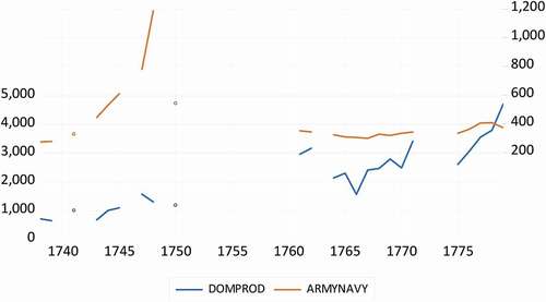
Suppose one is interested in any correlation or regression relation between these two variables. One approach could now be to simply ignore the missing data and compute the correlation or run a regression. This simple solution could work well, but in case the data show autocorrelation, that is, the data in year T-1 are informative for the data year T; then, the number of missing observations may be an obstacle for analysis. Indeed, when there are just three observations, $y_1,y_2,y_3$ and suppose $y_2$ is missing then this means that one simply cannot compute a first-order autocorrelation.

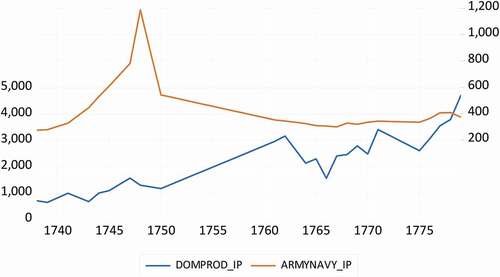
An often consider alternative is to interpolate the missing observations using the adjacent observed observations. For the missing $y_2$ above, this would entail that it is replaced by $y_2^{\ast }$, which is a function of $y_1$ and $y_3$. With this replaced value, one does have information to compute the first-order autocorrelation. Frequently, researchers choose a linear interpolation scheme, and this results in data like those in Figure 2, which displays some straight lines between various points. For another example, consider Figure 8A in O’Rourke and Jeffrey (2002).

Figure 2. The contribution to Gross Domestic Product in Holland (in 1000 guilders) for the Army and Navy.

In this paper, I will show that there is downside to interpolation and that is that it changes the autocorrelation structure of the time series. Next, ignoring such autocorrelation in subsequent correlation or regression analysis can lead to spurious results. A simple method is presented to prevent spurious results. A detailed illustration to the abovementioned two time series highlights the main issues.

II. Correlation and interpolation

Consider again the two time series in Figure 1, and suppose we are interested in measuring the relationship between these two variables. The data are observed for 1738–1779, and as is clear from Figure 1, there are many missing observations. Given the time span, there could have been 42 annual observations, but the number of effective observations is 24.

The estimated correlation between these two variables is −0.269. When we consider a simple regression model and apply Ordinary Least Squares (OLS) to

$DPT{S}_t=\alpha +\beta A{N}_t+{\epsilon }_t$

We obtain the estimation results

$a=2834\left(531.9\right)$

$b=-1.494\left(0.713\right)$

where the numbers in parentheses are the HAC standard errors (Heteroscedasticity and Autocorrelation Consistent). The estimated t-statistic on b is −2.097, and hence, there seems to be a significant relationship, with a p value of 0.048. There does seem to be some autocorrelation in the estimated residuals as the Eviews package gives a Durbin Watson test statistic value of 0.216, which is closer to 0 than to 2 (the value if there is no autocorrelation).

We may now want to increase the effective sample size from 24 to 42 by interpolating the missing observations. An often-applied technique is to draw a straight line between the begin and end points of a period with missing data, and the use the points on that line as the new observations. For example, suppose there are three observations $y_1,y_2,y_3$, and suppose the observation on $y_2$is missing. One can then decide to insert for $y_2$:

$y_1+\frac{1}{2}\left(y_3-y_1\right)=\frac{1}{2}{y}_1+\frac{1}{2}{y}_3$

In general, if there are $m-1$ missing observations in between any $y_1$ and $y_{m+1}$, then the interpolation scheme is

$y_1+\frac{1}{m}\left(y_{m+1}-y_1\right)=\frac{m-1}{m}{y}_1+\frac{1}{m}{y}_{m+1}$

$\frac{m-2}{m}{y}_1+\frac{2}{m}{y}_{m+1}$

to

$\frac{1}{m}{y}_1+\frac{m-1}{m}{y}_{m+1}$

If this scheme is applied to the two variables with 42–24 = 18 missing observations, we obtain the data as depicted in Figure 2.

The correlation between these two interpolated series is −0.333, a slight increase relative to the −0.269 before, at least in an absolute sense. When we consider a simple regression model to these interpolated series, and apply OLS to

$DPTS\mathrm{\_}interpolate{d}_t=\alpha +\beta AN\mathrm{\_}interpolate{d}_t+{\epsilon }_t$

We obtain the estimation results

$a=2924\left(534.0\right)$

$b=-1.817\left(0.773\right)$

where the numbers in parentheses are again the HAC standard errors. The estimated t-statistic on b is now −2.351, and hence, there seems to be a significant relationship, now even with a p value of 0.024. The Durbin Watson test statistic value for the 42 estimated residuals is 0.186, which is even closer to 0 and further away from 2.

The question now is whether this correlation and this relation is a statistical artefact. We seem to miss out on first-order autocorrelation, given the small Durbin Watson values, and also after interpolation, the first-order autocorrelation seems to increase.

To see if there is autocorrelation in each of the variables, we compute the first-order autocorrelation like

$r_1=\frac{\frac{1}{T}{\sum }_{t=1739}^{t=1789}\left(y_t-\bar{y}\right)(y_{t-1}-\bar{y})}{\frac{1}{T}{\sum }_{t=1739}^{t=1789}{(y_t-\bar{y})}^2}$

and also the second- to fifth-order autocorrelations. These estimates are displayed in Table 1. Comparing the columns with raw data and interpolated data, it is evident that the interpolated data have much more autocorrelation. In fact, the first-order autocorrelation seems to approach 1, which is the case of the so-called unit root, in which case one needs to resort to cointegration analysis, as is done in for example O’Rourke and Jeffrey (2002).

Table 1. Autocorrelations in the various variables, computed using

Lag i	DPTS	DPTS Interpolated	AN	AN Interpolated
1	0.521	0.821	0.433	0.825
2	0.454	0.709	0.268	0.613
3	0.295	0.586	0.323	0.471
4	0.236	0.513	0.148	0.326
5	0.232	0.470	0.086	0.187

¹Before we turn to correlation and regression analysis, we first examine the potential consequences of interpolation for the time series.

III. What does interpolation do?

To understand what interpolation does to the time series properties of variables, consider the following very simple and stylized case. Consider the following four observations:

${\epsilon }_1,{\epsilon }_2,{\epsilon }_3,{\epsilon }_4$

and assume that each of these four observations is a draw from a white noise process, that is they have mean zero, variance ${\sigma }^2$, and they are uncorrelated, that is, the correlation between any ${\epsilon }_i$ and ${\epsilon }_j$ for $i\ne j$ is zero. It is now easy to derive that

$r_1=\frac{\frac{1}{3}{\sum }_{t=2}^{t=4}({\epsilon }_t{\epsilon }_{t-1})}{\frac{1}{3}{\sum }_{t=2}^{t=4}{({\epsilon }_t)}^2}=\frac{0}{{\sigma }^2}=0$

Next, we consider three distinct cases when one or two observations can be missing. We use the linear interpolation technique, but for alternative methods, qualitatively similar results can be obtained, although the notation and mathematical expressions quickly become involved.

Case a: ${\epsilon }_2$ is missing and is interpolated using ${\epsilon }_1$ and ${\epsilon }_3$

In this case, the data series becomes

${\epsilon }_1,\frac{1}{2}{\epsilon }_1+\frac{1}{2}{\epsilon }_3,{\epsilon }_3,{\epsilon }_4$

Call these observations ${\epsilon }_t^{\ast }$

For this data series, it holds that

$\frac{1}{3}\sum _{t=2}^{t=4}({\epsilon }_t^{\ast }{\epsilon }_{t-1}^{\ast })=\frac{1}{3}\left(\frac{1}{2}{\sigma }^2+\frac{1}{2}{\sigma }^2+0\right)=\frac{1}{3}{\sigma }^2$

and that

$\frac{1}{3}\sum _{t=2}^{t=4}({\epsilon }_t^{\ast }{)}^2=\frac{1}{3}\left(\frac{1}{4}{\sigma }^2+\frac{1}{4}{\sigma }^2+{\sigma }^2+{\sigma }^2\right)=\frac{5}{6}{\sigma }^2$

Hence, the first-order autocorrelation becomes

$r_1=\frac{\frac{1}{3}{\sum }_{t=2}^{t=4}({\epsilon }_t^{\ast }{\epsilon }_{t-1}^{\ast })}{\frac{1}{3}{\sum }_{t=2}^{t=4}{({\epsilon }_t^{\ast })}^2}=\frac{\frac{1}{3}}{\frac{5}{6}}=\frac{2}{5}=0.4$

So, the first-order autocorrelation quickly jumps from 0 to 0.4.

Case b: ${\epsilon }_2$ and ${\epsilon }_3$ are missing and are interpolated using ${\epsilon }_1$ and ${\epsilon }_4$

When there are two observations missing, the linear interpolation method results in the new observations

${\epsilon }_1,\frac{2}{3}{\epsilon }_1+\frac{1}{3}{\epsilon }_4,\frac{1}{3}{\epsilon }_1+\frac{2}{3}{\epsilon }_4,{\epsilon }_4$

We now have that

$\frac{1}{3}\sum _{t=2}^{t=4}({\epsilon }_t^{\ast }{\epsilon }_{t-1}^{\ast })=\frac{1}{3}\left(\frac{2}{3}{\sigma }^2+\frac{2}{9}{\sigma }^2+\frac{2}{9}{\sigma }^2+\frac{2}{3}{\sigma }^2\right)=\frac{16}{27}{\sigma }^2$

and that

$\frac{1}{3}\sum _{t=2}^{t=4}({\epsilon }_t^{\ast }{)}^2=\frac{1}{3}\left(\frac{5}{9}{\sigma }^2+\frac{5}{9}{\sigma }^2+{\sigma }^2\right)=\frac{19}{27}{\sigma }^2$

which makes the first-order autocorrelation to become

$r_1=\frac{\frac{1}{3}{\sum }_{t=2}^{t=4}({\epsilon }_t^{\ast }{\epsilon }_{t-1}^{\ast })}{\frac{1}{3}{\sum }_{t=2}^{t=4}{({\epsilon }_t^{\ast })}^2}=\frac{16}{19}\cong 0.84$

The differences between cases a and b are that, as could be expected, the variance decreases (from $\frac{5}{6}{\sigma }^2$ to $\frac{19}{27}{\sigma }^2$), and that the first-order autocorrelation increases (from 0.4 to 0.84).

Case c: ${\epsilon }_2$ is missing and is interpolated using ${\epsilon }_1$ and ${\epsilon }_3$, while there are five observations, that is, one more than case a.

In this case, we thus have

${\epsilon }_1,\frac{1}{2}{\epsilon }_1+\frac{1}{2}{\epsilon }_3,{\epsilon }_3,{\epsilon }_4,{\epsilon }_5$

which gives

$\frac{1}{4}\sum _{t=2}^{t=5}({\epsilon }_t^{\ast }{\epsilon }_{t-1}^{\ast })=\frac{1}{4}\left(\frac{1}{2}{\sigma }^2+\frac{1}{2}{\sigma }^2+0+0\right)=\frac{1}{4}{\sigma }^2$

and

$\frac{1}{4}\sum _{t=2}^{t=5}({\epsilon }_t^{\ast }{)}^2=\frac{1}{4}\left(\frac{1}{4}{\sigma }^2+\frac{1}{4}{\sigma }^2+{\sigma }^2+{\sigma }^2+{\sigma }^2\right)=\frac{7}{8}{\sigma }^2$

resulting in

$r_1=\frac{\frac{1}{4}{\sum }_{t=2}^{t=5}({\epsilon }_t^{\ast }{\epsilon }_{t-1}^{\ast })}{\frac{1}{4}{\sum }_{t=2}^{t=5}{({\epsilon }_t^{\ast })}^2}=\frac{2}{7}\cong 0.29$

So, when the number of non-interpolated data decreases, the first-order autocorrelation also decreases.

IV. What does neglected autocorrelation do?

Already in Udny (1926), the issue of spurious correlation was raised, which basically occurs due to neglected autocorrelation. When the data have trends, Granger and Newbold (1974) showed that high-valued nonsense correlations can occur. In Phillips (1986), it was shown that for trended data such nonsense correlations can be obtained when people rely on inappropriate statistical methodology. Later, Granger, Hyung, and Jeon (2001) derived the asymptotic distribution of the t test on the parameter $\beta$ in the simple regression

$y_t=\alpha +\beta x_t+{\epsilon }_t$

where in reality

$y_t=\rho y_{t-1}+u_t$

$x_t=\rho x_{t-1}+w_t$

that is, the two variables are independent first-order autoregressive time series with the same parameter $\rho$. This asymptotic distribution is

$t_{\beta }\sim N\left(0,\frac{1+{\rho }^2}{1-{\rho }^2}\right)$

instead of the commonly considered $N\left(0,1\right)$ distribution. Clearly,

$\frac{1+{\rho }^2}{1-{\rho }^2}>1$

and hence, more often significant test values will be found. Indeed, Table 5A.1 in Franses (2018) shows that when for example $\rho =0.7$, one will obtain around 23% significant t test values. And, in this case, the average absolute correlation between $y_t$ and $x_t$ is 0.131 for 100 observations, and as large as 0.248 for 25 observations.

In sum, neglected autocorrelation leads to spurious relations.

V. How to prevent spurious results?

A simple remedy to prevent spurious results is to explicitly incorporate lags of the variables. In our illustrative example, this means that we move from

$DPTS\mathrm{\_}interpolate{d}_t=\alpha +\beta AN\mathrm{\_}interpolate{d}_t+{\epsilon }_t$

to

$DPTS\mathrm{\_}interpolate{d}_t=\alpha +\beta AN\mathrm{\_}interpolate{d}_t+\gamma DPTS\mathrm{\_}interpolate{d}_{t-1}+{\epsilon }_t$

The OLS estimation results for this extended model are

$a=179.3\left(206.8\right)$

$b=-0.141\left(0.229\right)$

$c=0.990\left(0.085\right)$

Clearly, the parameter for Army Navy is now insignificant.

Given the high-valued autocorrelations in Table 1, and also given the estimate of 0.990 for $c$, one can also correlate the differences of the two variables, thereby imposing that each of the two has a unit root. Then, the regression becomes

$DPTS\mathrm{\_}interpolate{d}_t-DPTS\mathrm{\_}interpolate{d}_{t-1}=\alpha +\beta \left(AN\mathrm{\_}interpolate{d}_t-AN\mathrm{\_}interpolate{d}_{t-1}\right)+{\epsilon }_t$

and the OLS estimation results (with HAC standard errors) are

$a=97.76\left(53.28\right)$

$b=-0.082\left(0.247\right)$

Clearly, there is no significant link between the two differenced variables.

VI. Conclusion

When analysing historical time series with missing observations, it is a common practice either to ignore these missing values or otherwise to interpolate between the adjacent observations and continue with the interpolated data as true data. In this paper, we have shown that interpolation changes the autocorrelation structure of the time series. Ignoring such autocorrelation in subsequent correlation or regression analysis could lead to spurious results. A simple method was presented to prevent spurious results. A detailed illustration highlighted the main issues and showed that presumably none-zero correlation disappears when the data are analysed properly.

Further research should indicate how often spurious correlations appear in historical research.

$r_i=\frac{\frac{1}{T}{\sum }_{t=1738+i}^{t=1789}\left(y_t-\bar{y}\right)(y_{t-i}-\bar{y})}{\frac{1}{T}{\sum }_{t=1738+i}^{t=1789}{(y_t-\bar{y})}^2}$

Disclosure statement

No potential conflict of interest was reported by the author(s).

Notes

¹ The data source is Brandon, P. and U. Bosma (2019), Calculating the weight of slave-based activities in the GDP of Holland and the Dutch Republic – Underlying methods, data and assumptions, The Low Countries Journal of Social and Economic History, 16 (2), 5–45, doi: 10.18352/tseg.1082

References

- Franses, P. H. 2018. Enjoyable Econometrics. Cambridge UK: Cambridge University Press.
- Granger, C. W. J., N. Hyung, and Y. Jeon. 2001. “Spurious Regressions with Stationary Series.” Applied Economics 33 (7): 899–904. doi:https://doi.org/10.1080/00036840121734.
- Granger, C. W. J., and P. Newbold. 1974. “Spurious Regression in Economics.” Journal of Econometrics 2 (2): 111–120. doi:https://doi.org/10.1016/0304-4076(74)90034-7.
- O’Rourke, K. H., and G. W. Jeffrey. 2002. “When Did Globalization Begin?” European Review of Economic History 6 (1): 23–50. doi:https://doi.org/10.1017/S1361491602000023.
- Phillips, P. C. B. 1986. “Understanding Spurious Regressions in Econometrics.” Journal of Econometrics 33 (3): 311–340. doi:https://doi.org/10.1016/0304-4076(86)90001-1.
- Udny, Y. G. 1926. “Why Do We Sometimes Get Nonsense Correlations between Time Series? A Study in Sampling and the Nature of Time Series.” Journal of the Royal Statistical Society 89 (1): 1–64. doi:https://doi.org/10.2307/2341482.