Performance analysis of nowcasting of GDP growth when allowing for conditional heteroscedasticity and non-Gaussianity

ABSTRACT

The nowcasting performance of autoregressive models for GDP growth are analysed in a setting where the error term is allowed to be characterized both by conditional heteroscedasticity and non-Gaussianity. Standard, publicly available, quarterly data on GDP growth from 1979 to 2019 for six countries are employed: Australia, Canada, France, Japan, the United Kingdom and the United States. In-sample analysis suggests that when homoscedasticity is assumed, support is provided for non-Gaussian error terms; the estimated degrees of freedom of the t-distribution lie between two and seven for all countries. However, allowing for both conditional heteroscedasticity and t-distributed innovations, results indicate that conditional heteroscedasticity captures the fat-tailed behaviour of the data to a large extent. Results from out-of-sample analysis show that point nowcasts are hardly affected by taking conditional heteroscedasticity and/or non-Gaussianity into account. For the density nowcasts, it is found that accounting for conditional heteroscedasticity leads to improvements for Australia, Canada, Japan, the United Kingdom and the United States; allowing for non-Gaussianity seems less important though. This result is robust to which measure is used for assessing density nowcasting performance.

KEYWORDS:

• GARCH
• Kullback-Leibler divergence
• non-Gaussianity
• probability integral transform

JEL Classification:

• E17
• E37

I. Introduction

Gross domestic product (GDP) growth is one of the macroeconomic aggregates that receives most attention by financial markets, policy makers and other economic agents. There is accordingly an extremely voluminous literature concerned with the issue of predicting GDP growth.¹ An overwhelming majority of this research has been directed at generating good point forecasts. However, a smaller but growing literature has focused on the issue of predictive densities for GDP growth; significant contributions have been made by, for example, Aastveit et al. (2014), Mazzi, Mitchell, and Montana (2014) and Carriero and Clark (2015). Density forecasts have also become an important tool in a policy setting for more than two decades now, as manifested in, for example, fan charts, for inflation (and other variables) generated by central banks such as the Bank of England and Sveriges Riksbank.² Recently, the issue of the shape and variance of the predictive distribution has received even more attention as the International Monetary Fund has lifted the concept of growth-at-risk in many of its reports, thereby providing a statement regarding the probability of poor outcomes for GDP growth.³ Predictive densities seem to be of growing importance in policy environments – not only as an issue for external communication but also as an input in the policy process – and it seems likely that the economic crisis following the corona pandemic will further strengthen this development.

If one is concerned about issues such as the likelihood of unusually low GDP growth, it seems relevant to consider two facts regarding macroeconomic time series, namely i) that they seem to benefit from being modelled with time-varying volatility in the disturbances – see, for example, Fountas and Karanasos (2007), Hamilton (2010), Pontines (2010), Clark (2011), Carriero and Clark (2015), Trypsteen (2017), Karlsson and Österholm (2020) and Kiss and Österholm (2021) – and ii) that data appear to have fat tails as pointed out by, for example, Christiano (2007), (Fagiolo, Napoletano, and Roventini (2008) and Ascari, Fagiolo, and Roventini (2015) and Kiss and Österholm (2020).⁴ The existence of fat tails in the data means that one might want to consider abandoning the traditional assumption of normally distributed disturbances and instead rely on a distribution with heavier tails, such as the t-distribution. However, as was pointed out already by Engle (1982) and Bollerslev (1986) in their seminal contributions on ARCH (autoregressive conditional heteroscedasticity) and GARCH (generalized autoregressive conditional heteroscedasticity) models, heavy tails might be due to time-varying volatility of the disturbances. This means that it is not obvious whether one should abandon the assumption of normality when estimating a model with time-varying volatility; whether that is worth doing is an empirical question.

To address this question, the empirical relevance of time-varying volatility (captured by conditional heteroscedasticity) and non-Gaussianity is assessed by analysing time series of real GDP growth for six countries: Australia, Canada, France, Japan, the United Kingdom and the United States. Using quarterly data from 1979 to 2019, in-sample analysis is first conducted where univariate autoregressive (AR) models with different assumptions regarding the disturbances of the model are estimated; homoscedastic models and GARCH models are used assuming disturbances drawn from either a normal distribution or a t-distribution. The four different models which are estimated for each country are then used in an out-of-sample nowcasting exercise where both the point and density nowcasts from the models are evaluated. Our focus on nowcasting – that is, the task of predicting output growth of the current quarter – is not unique. In fact, it is a field that has gained significant attention over the last decade; contributions include Giannone, Reichlin, and Small (2008), Angelini et al. (2011), Banbura, Giannone, and Reichlin (2011), Kuzin, Marcellino, and Schumacher (2011), Aastveit et al. (2014), Girardi, Gayer, and Reuter (2016), Jansen, Jin, and de Winter (2016), Madhou et al. (2017) and Cepni, Guney, and Swanson (2020). Moreover, having a short forecast horizon is also beneficial from an evaluation perspective; it allows us to circumvent problems such as the presence of serial correlation due to the overlapping nature of the forecast error at longer forecast horizons. Using longer horizons results in a considerable decrease in the number of independent errors to evaluate; this leads to less statistical power, and hence a loss of precision of the density forecast evaluation measures.

In conducting this analysis, two distinct contributions to the literature are made. These contributions aim to address a gap in the empirical macroeconomic literature, namely that there is limited knowledge as to whether – and to which extent – GDP growth is characterized by heavy tails and how that might impact nowcasting performance; this area is still largely unexplored, which is somewhat surprising given the fact that deviations from normality might have substantial consequences, in particular, for density nowcast evaluation.⁵ As a first contribution, further international empirical evidence is added regarding the relevance of conditional heteroscedasticity and non-Gaussian error terms when modelling real GDP growth data. As a second contribution, the point and density nowcasting performance of models with and without fat tails is evaluated. Accordingly, relevant information is provided as to whether it is worth abandoning the assumption of independent, identically normally distributed error terms in favour of conditional heteroscedasticity and/or non-Gaussian error terms when modelling and nowcasting GDP growth. Also, it should be stressed that our contributions are not only relevant from an academic perspective, but they are also important for practitioners. Both point and density nowcasts are important inputs for economic policy; hence, assessing and improving the statistical properties of these nowcasts might result in more refined policy decisions.

Briefly summarizing our results, in-sample it is found that all countries have relatively mild serial correlation in the first moment, which is largely unaffected by the modelling assumptions of the error terms. For models assumed to be homoscedastic, support is typically found for non-Gaussian error terms; the estimated degrees of freedom of the t-distribution lie between two and seven for all countries. Data support the modelling of conditional heteroscedasticity, except for France. However, results based on allowing for both conditional heteroscedasticity and t-distributed innovations suggest that conditional heteroscedasticity captures the fat-tailed behaviour of the data to a large extent. Exceptions are the United Kingdom and the United States where the distribution of the error term remains heavy tailed (degrees of freedom close to four and five for the t-distribution, respectively) even after controlling for conditional heteroscedasticity.

The out-of-sample results indicate that point nowcasts – and hence the nowcast precision of the models – are materially unaffected by allowing for more general assumptions concerning the error term. Turning to density nowcasts, it can first be noted – perhaps somewhat surprisingly – that assuming a t-distribution rather than a normal in a homoscedastic model does not seem to generate improvements in general. In contrast, accounting for conditional heteroscedasticity improves density nowcasts in Australia, Canada, the United Kingdom, and the United States. It seems that it mostly suffices to take conditional heteroscedasticity into account; assuming a t-distribution (rather than a normal) for the error term does not lead to large further improvements in the density nowcasts.

The remainder of this paper is organized as follows: In SectionII, data are described and some descriptive statistics are provided. Section III introduces the methodological framework that the empirical analysis relies upon. In Section IV, results are presented and findings are discussed. Finally, Section V concludes.

II. Data

The main focus of our analysis is the quarterly real GDP growth series, $g_t$, which is defined as $g_t=100\frac{Y_t-Y_{t-1}}{Y_{t-1}}$, where $Y_t$ is seasonally adjusted real GDP. Data from six member countries of the Organisation for Economic Co-operation and Development (OECD) are employed: Australia, Canada, France, Japan, the United Kingdom and the United States.⁶ The data used have been supplied by the statistical office of the respective country (accessed through the Macrobond data provider). The validity of our data is established by the fact that developed countries are analysed, whose production of statistics all conform with the strict international standards regarding the production of official statistics. With one exception (Japan), the samples span the time period 1979Q3 to 2019Q3⁷ – a choice based mainly on data availability.⁸, ⁹ Data are shown in Figure 1.

Figure 1. GDP growth series.

Note: Percent on vertical axes.

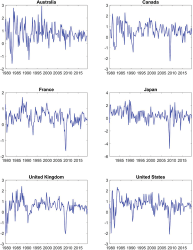
Looking at the data, there are signs of volatility clustering and to some extent these tend to be common across countries. For example, several countries have a somewhat higher volatility in the beginning of the sample, though Japan does not show this pattern. And of course, the global financial crisis of 2008 was associated with large movements, with the exception of Australia, which shows a gradual decrease in volatility during the sample. It is admittedly not trivial though to see whether there is conditional heteroscedasticity which is why this issue is formally investigated in Section III.

Concerning the issue of whether the data are characterized by fat tails, some descriptive statistics of the output growth series are first provided. Figure 2 plots histograms of our data by country. Even though the number of observations is limited, the shape of the distribution of output growth indicates fat tails in each of the countries. This is also confirmed by the descriptive statistics in Table 1. The kurtosis values for each of the countries suggest a leptokurtic distribution; in addition, negative skewness is present in five out of the six countries considered. The null hypothesis of the Jarque-Bera test (Jarque and Bera 1980) of normality, which is based on the skewness and the kurtosis of the series, is also strongly rejected for each country. Therefore, in line with what was established for a number of OECD countries by Fagiolo, Napoletano, and Roventini (2008), it is concluded that the unconditional distribution of the output growth series is non-normally distributed. In particular, it is characterized by heavy tails, which one likely wants to account for when forming density nowcasts.

Figure 2. Histograms of GDP growth rates.

Note: Number of observations in each bin on vertical axes. Percent on horizontal axes.

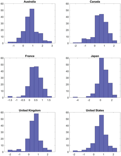
Table 1. Descriptive statistics and Jarque-Bera test statistic

Country	Mean	Variance	Skewness	Kurtosis	Jarque-Bera
Australia	0.771	0.517	0.035	4.047	7.40
Canada	0.586	0.538	−0.697	4.190	22.53
France	0.446	0.214	−0.791	6.284	89.12
Japan	0.473	0.978	−0.918	7.455	152.82
United Kingdom	0.515	0.494	−1.112	6.540	117.25
United States	0.664	0.492	−0.867	5.561	64.15

Note: The critical value at the five percent level of the Jarque-Bera test is 5.99.

III. Methodological framework

An empirical analysis of the data is conducted both in- and out-of-sample; for the out-of-sample analysis, both point and density nowcasts are evaluated. The nowcasting models that are employed are univariate and more specifically given by a first order autoregressive [AR(1)] model. This is based on the fact that the univariate model, and in particular, the AR(1) model, is a very commonly used benchmark in the macroeconomic literature which tends to forecast reasonably well; see, for example, Pesaran, Schuermann, and Smith (2009).¹⁰ It hence seems reasonable to choose a parsimonious model for the conditional mean. The stylized fact that output growth series tend to be weakly serially correlated – further confirmed by our analysis – lends further support for a parsimonious specification of the conditional mean.¹¹ When modelling volatility, what can be described as a robust approach is chosen – namely to rely on the GARCH(1,1) model. This is a common benchmark in volatility modelling – see, for example, Chung et al. (2012) and Clark and Ravazzolo (2015) in the macroeconomic context – and there are indications that, at least for financial data, it is a modelling choice quite difficult to beat; see, for example, Hansen and Lunde (2005). Furthermore, the GARCH specification nests simpler specifications, such as ARCH(1) or constant conditional volatility, thereby allowing us to flexibly capture patterns in volatility.

Two main models are accordingly specified. The first of these is the ‘homoscedastic AR(1) model’. This is given as

(1) $g_t={\gamma }_0+{\gamma }_1{g}_{t-1}+{\sigma }_{\nu }{\nu }_t$(1)

where $g_t$ is real GDP growth and ${\nu }_t$ is assumed to be either drawn from a normal distribution or a t-distribution. That is, it is assumed that ${\nu }_t\text{~}N\left(0,1\right)$ or ${\nu }_t\text{~}t\left(\kappa \right)$ where $\kappa$ is the degrees of freedom.

The second model is the AR(1)-GARCH(1,1) model:

(2) $g_t={\gamma }_0+{\gamma }_1{g}_{t-1}+{\epsilon }_t$(2)

(3) ${\epsilon }_t={\sigma }_t{v}_t$(3)

(4) ${\sigma }_t^2=\omega +\alpha {\epsilon }_{t-1}^2+\beta {\sigma }_{t-1}^2$(4)

where $g_t$ is real GDP growth and $v_t$ is assumed to be an iid error term distributed according to a normal distribution or a t-distribution with $\kappa$ degrees of freedom, as above. Given two different models and two different assumptions regarding the distribution of the error term, there are, in total, four models that are estimated, analysed and evaluated.

Estimation of the models is performed by conditional maximum likelihood. The in-sample evaluation of the models is based on full-sample parameter estimates and the corresponding maximum likelihood standard errors are calculated according to the usual outer product gradient method. The out-of-sample analysis has a dual focus, on both point and density nowcasts. The point nowcasts are evaluated based on the root mean square error (RMSE) of the nowcast, calculated as

(5) $RMSE=\sqrt{\frac{1}{N}{\mathrm{\Sigma }}_{{ }_{t=1}}^n{\left(g_t-g_{t|t}\right)}^2}$(5)

where $g_t$ (as above) is real GDP growth at quarter t, $g_{t|t}$ is the nowcast (assumed to be generated standing partway through the quarter) and N is the number of nowcasts evaluated.¹² To compare point nowcasting accuracy, the Diebold-Mariano test (Diebold and Mariano 1995) is used. The test statistic is based on the squared error differential of two specifications, a and b,

(6) $d_t={\left(g_t-g_{t|t}^a\right)}^2-{\left(g_t-g_{t|t}^b\right)}^2,$(6)

and can be written as

(7) $DM=\frac{\bar{d}}{{\sigma }_d/\sqrt{N}},$(7)

where $\bar{d}$ and ${\sigma }_d$ are the sample mean and standard deviation of the squared error differentials, respectively. A positive test statistic means that model b outperforms model a in terms of point nowcast accuracy. Under the null of equal nowcasting performance, the test statistic is distributed as standard normal.¹³

In terms of density nowcast evaluation, the analysis is based on the probability integral transform (PIT) as proposed by Diebold, Gunther, and Tay (1998). Let $f_t$ be the density nowcast. Then

(8) $z_t={\int }_{-\mathrm{\infty }}^{y_t}{f}_t\left(x\right)dx=F_t\left(y_t\right)$(8)

is the PIT of the process, that is, the realized observations are transformed by the cumulative distribution function implied by the density nowcast. The idea is that if the nowcast density is the one implied by the true data-generating process, then the PIT values are independent and identically uniformly distributed on the interval [0,1]. Hence, density nowcasts can be evaluated according to how close to iid uniform is the distribution of the PIT they produce.

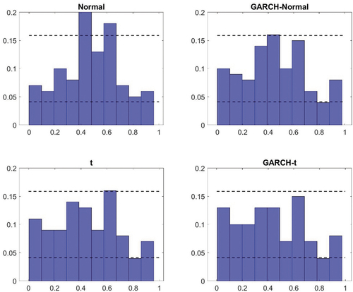
A common procedure – as also suggested by Diebold, Gunther, and Tay (1998) – for evaluating the uniformity of the PIT is simply a visual inspection of the histograms. It is usually accompanied by a more formal test: confidence intervals for the bin height of the histogram obtained under the null that the data are generated by a uniform distribution. Even though the approach is formally valid, it can often be difficult to draw meaningful inference using this approach. The confidence intervals for the bins under the null of a uniform distribution are usually wide (if the number of observations is relatively low as in the present case), which implies low statistical power against the null of uniformity. In addition, it can also be hard to compare two density nowcasts based on the PIT histograms they produce. Given this difficulty, the Kullbach-Leibler (KL) divergence of the PIT series from an iid uniform distribution is proposed as a summary measure.¹⁴ The general definition of the KL divergence for a distribution is

(9) $KL=-{\int }_{-\mathrm{\infty }}^{\mathrm{\infty }}p\left(x\right)log\left(\frac{q\left(x\right)}{p\left(x\right)}\right)dx$(9)

where $p\left(x\right)$ is the target density and $q\left(x\right)$ is the density being compared to the target. In practice, the KL measure is based on the histograms of the PIT and the uniform distribution. A higher value for KL divergence means that the distribution of the PIT is further away from the uniform distribution, meaning that the model with the smallest KL has generated the best density nowcast.

Formal statistical tests of uniformity of the PIT series are also conducted.¹⁵ Goodness-of-fit tests operate under the null hypothesis that the observations come from a pre-specified distribution – uniform on the interval [0,1] in case of the PIT. Two of the most commonly used tests based on the cumulative distribution function of the observations are the Kolmogorov–Smirnov (KS) and the Anderson–Darling (AD) tests – both defined, for example, in Anderson and Darling (1952). To give a formal definition of the tests consider $\mathrm{\Psi }\left(\mathrm{r}\right)=I\left(z_t<r\right)-r$ as the distance between the empirical cumulative distribution function of the PIT from the uniform distribution at a given quantile $r$, and $\overline{\Psi }\left(r\right)$ as its mean in the out-of-sample nowcasting sample. The test statistics can be written as

(10) $KS=\underset{r}{sup}\left|\bar{\mathrm{\Psi }}\left(r\right)\right|,$(10)

(11) $AD=01\frac{{\bar{\mathrm{\Psi }}}^2\left(r\right)}{r\left(1-r\right)}dr.$(11)

If the PIT is indeed uniformly distributed, both the KS and the AD statistics are close to zero. Both tests are one-sided and a higher value for both test statistics therefore implies that the distribution is further away from the null.¹⁶ Hence, one can simply compare two nowcasts based on these test statistics and interpret a lower value for the test statistic as a better density nowcast.

IV. Results

As described above, the main aim is to assess how conditional heteroscedasticity and non-Gaussianity can affect nowcasting performance in the context of GDP growth. Results are presented from four different specifications: i) the benchmark model with constant volatility and normally distributed innovations, ii) a model with constant volatility and t-distributed innovations, iii) a model with conditional heteroscedasticity and normally distributed errors, and iv) a specification allowing for both conditional heteroscedasticity and t-distributed error terms. By comparing these four specifications, the relative importance of each factor can be investigated. Results from in-sample estimation and out-of-sample nowcasting are shown for all six countries.

In-sample results

The parameter estimates for the models and the corresponding p-values are presented in Table 2. The results for the mean equation are in line with the usual findings in the literature: The growth series are mildly serially correlated; the AR(1) coefficients are in the range between 0 and 0.55 regardless of the underlying assumptions on the disturbances.

Table 2. In-sample estimation results

		Australia				Canada
		(1)	(2)	(3)	(4)	(1)	(2)	(3)	(4)
Mean equation [AR(1)]	${\gamma }_0$	0.603	0.604	0.619	0.620	0.291	0.280	0.349	0.348
		(0.000)	(0.000)	(0.000)	(0.000)	(0.000)	(0.000)	(0.000)	(0.000)
	${\gamma }_1$	0.218	0.196	0.121	0.119	0.502	0.536	0.403	0.425
		(0.001)	(0.002)	(0.118)	(0.117)	(0.000)	(0.000)	(0.000)	(0.000)
GARCH equation	$\omega$			<0.000	<0.000			0.130	0.113
				(0.999)	(0.999)			(0.007)	(0.088)
	$\alpha$			0.059	0.058			0.364	0.358
				(0.076)	(0.114)			(0.019)	(0.040)
	$\beta$			0.932	0.932			0.330	0.384
				(0.000)	(0.000)			(0.096)	(0.136)
Degrees of freedom	$\kappa$		5.611		22.050		6.291		12.181
			[3.354]		[37.675]		[3.319]		[10.604]
ARCH-test		10.973	11.212	1.103	1.097	6.834	5.906	0.671	0.918
		(0.027)	(0.024)	(0.894)	(0.895)	(0.145)	(0.206)	(0.955)	(0.922)
JB-test		6.708	0.421^a	0.534	0.002^a	13.684	0.470^a	7.354	2.166^a
		(0.035)	(>0.500)	(>0.500)	(>0.500)	(0.007)	(>0.500)	(0.029)	(0.339)
T		161	161	161	161	161	161	161	161
		France				Japan*
		(1)	(2)	(3)	(4)	(1)	(2)	(3)	(4)
Mean equation [AR(1)]	${\gamma }_0$	0.207	0.248	0.230	0.241	0.386	0.430	0.402	0.405
		(0.000)	(0.000)	(0.000)	(0.000)	(0.000)	(0.000)	(0.000)	(0.000)
	${\gamma }_1$	0.536	0.474	0.492	0.478	0.181	0.134	0.160	0.162
		(0.000)	(0.000)	(0.000)	(0.000)	(0.000)	(0.025)	(0.061)	(0.066)
GARCH equation	$\omega$			0.051	0.064			0.438	0.440
				(0.290)	(0.417)			(0.001)	(0.002)
	$\alpha$			0.173	0.128			0.546	0.541
				(0.150)	(0.280)			(0.001)	(0.003)
	$\beta$			0.496	0.442
				(0.193)	(0.427)
Degrees of freedom	$\kappa$		6.687		9.916		4.856		38.519
			[3.790]		[8.688]		[1.839]		[137.340]
ARCH-test		8.926	9.859	7.120	6.619	27.785	23.724	2.326	2.246
		(0.063)	(0.042)	(0.130)	(0.157)	(0.000)	(0.000)	(0.676)	(0.691)
JB-test		14.102	2.284^a	4.505	1.186^a	75.542	1.988^a	1.095	0.786^a
		(0.007)	(0.319)	(0.078)	(>0.500)	(0.000)	(0.370)	(>0.500)	(>0.500)
T		161	161	161	161	158	158	158	158
		United Kingdom				United States
		(1)	(2)	(3)	(4)	(1)	(2)	(3)	(4)
Mean equation [AR(1)]	${\gamma }_0$	0.251	0.362	0.254	0.336	0.406	0.481	0.429	0.481
		(0.000)	(0.000)	(0.000)	(0.000)	(0.000)	(0.000)	(0.000)	(0.000)
	${\gamma }_1$	0.507	0.343	0.551	0.421	0.388	0.335	0.403	0.329
		(0.000)	(0.000)	(0.000)	(0.000)	(0.000)	(0.000)	(0.000)	(0.000)
GARCH equation	$\omega$			0.047	0.070			0.054	0.049
				(0.017)	(0.144)			(0.191)	(0.267)
	$\alpha$			0.213	0.402			0.153	0.210
				(0.011)	(0.146)			(0.004)	(0.086)
	$\beta$			0.642	0.510			0.700	0.684
				(0.000)	(0.003)			(0.000)	(0.000)
Degrees of freedom	$\kappa$		2.048		3.520		3.661		4.987
			[0.617]		[0.276]		[1.390]		[2.107)]
ARCH-test		14.134	21.041	1.274	1.085	31.558	26.806	4.278	2.386
		(0.007)	(0.000)	(0.866)	(0.897)	(0.000)	(0.000)	(0.370)	(0.665)
JB-test		24.809	38.338^a	23.198	2.766^a	51.019	4.808^a	56.434	3.054^a
		(0.002)	(0.000)	(0.002)	(0.251)	(0.000)	(0.090)	(0.000)	(0.217)
T		161	161	161	161	161	161	161	161

Note: The table presents estimation results of the univariate GDP nowcasting model. Model (1) assumes a conditionally homoscedastic standard normal distribution. Model (2) assumes a conditionally homoscedastic t-distribution. Model (3) allows for GARCH(1,1) error terms with standard normal innovations. Model (4) allows for GARCH(1,1) error terms with t-distributed innovations. Standard errors are calculated using the outer product gradient method. The ARCH test is Engle’s test for conditional heteroscedasticity (Engle 1982) using four lags, and the JB-test is the Jarque-Bera test for normality (Jarque and Bera 1980). “a” indicates that the Jarque-Bera test is performed on the probability integral transform of the (standardized) residuals (see footnote 17). T is the number of observations. p-values are in parentheses (). Standard errors for the degrees of freedom in brackets []^{. *} For Japan, the lower bound ($\beta =0$) becomes a binding constraint in the maximum likelihood estimation and no estimate for $\beta$ is accordingly reported.

Turning to the issue of the fat tails documented above, it can first be observed that one can reject normality of the residuals in each country in the benchmark model, which does not account for either conditional heteroscedasticity or non-Gaussianity. The statistic for the Jarque-Bera test of normality (Jarque and Bera 1980) lies between 6.8 and 77.2, which indicates a strong rejection of the null.

When estimating homoscedastic models, the results tend to favour finding non-Gaussian error terms, although results vary from country to country. The estimated degrees of freedom for a t-distribution lie between two and seven in all cases, with relatively low standard errors for Japan, the United Kingdom and the United States.

Looking at the estimated GARCH models, it can initially be noted that support for such a specification can be found in all countries except France. Comparing the two GARCH specifications for each country, parameter estimates do generally not differ a lot depending on whether a normal or t-distribution is used; the differences for the United Kingdom are non-negligible though. The estimated parameters also show that the persistence of the process for the variance – measured as $\alpha +\beta$ – is moderate and values range from approximately 0.6 to 0.9. The exception is Australia where the persistence is 0.99. This might be due to what appears to be a decreasing trend in the volatility which is picked up by the GARCH equation for the volatility. This explanation is further supported by the estimated conditional volatility in Figure A1 in the Appendix, which explicitly shows a downward trend in estimated volatility.

Finally, assuming a t-distribution for the error terms in the GARCH model seems to find support only in the United Kingdom and the United States. However, in both those cases, the standard errors are low and the estimated degrees of freedom are 3.5 and 5 respectively – that is, the tails of the error distribution are quite heavy even after controlling for conditional heteroscedasticity.

Formal tests for the conditional heteroscedasticity (Engle 1982) and the non-Gaussianity for the residuals of each model (Jarque and Bera 1980) are also conducted.¹⁷ Based on the former test, the GARCH(1,1) specification appears to capture all conditional heteroscedasticity. The Jarque-Bera test shows that a t-distribution captures non-Gaussianity well; even in the homoscedastic models, the test rejects normality only in the case of the United Kingdom. When also allowing for conditional heteroscedasticity, the null hypothesis that the transformed residuals are normally distributed cannot be rejected for any country.

Out-of-sample results

Using the four model specifications from above, parametric density nowcasts for output growth are next obtained. That is, the models are estimated on an expanding sample (expanding window), where the first nowcast is based on the sample 1979Q3-1994Q3 and a nowcast is generated for 1994Q4.¹⁸ The predictions and predictive densities (which are formed based on the estimated parameter values and the assumed distribution for the error term) from the four models are then compared to the actual value. Next, a quarter is added, all models re-estimated, new predictions and predictive densities generated (this time for 1995Q1) and new comparisons to the actual value are made. This continues until the end of the sample, where models are estimated on data from 1979Q3-2019Q2 and predictions and predictive densities generated for 2019Q3. Having done this, RMSEs are calculated according to Equation (5(5) $RMSE=\sqrt{\frac{1}{N}{\mathrm{\Sigma }}_{{ }_{t=1}}^n{\left(g_t-g_{t|t}\right)}^2}$(5) ) in order to assess the point nowcasting performance. The Diebold-Mariano test statistic is also presented, where the benchmark Gaussian, homoscedastic model is compared to the other specifications with more elaborate assumptions concerning the error term. A positive value means that the alternative error specification outperforms the benchmark.

The density nowcasting performance is evaluated using the PIT series calculated in Equation (8(8) $z_t={\int }_{-\mathrm{\infty }}^{y_t}{f}_t\left(x\right)dx=F_t\left(y_t\right)$(8) ), which are plotted for each country and each specification in Figure A2-A7 in the Appendix. The measures presented in Table 3 for density nowcast comparison are the Kullbach-Leibler divergence of the PIT from the uniform distribution and the Kolmogorov–Smirnov and Anderson–Darling statistics.

Table 3. Nowcast evaluation results for GDP growth

	Australia					Canada
Error	RMSE	DM	KL	KS	AD	RMSE	DM	KL	KS	AD
Normal	0.574	-	0.131	0.143	4.439	0.526	-	0.067	0.117	2.864
t	0.573	2.573	0.131	0.142	4.433	0.528	−0.230	0.094	0.108	2.245
GARCH-Normal	0.567	2.147	0.078	0.114	1.782	0.526	0.101	0.010	0.074	0.889
GARCH-t	0.567	2.177	0.078	0.114	1.738	0.526	0.173	0.015	0.074	0.913
	France					Japan
	RMSE	DM	KL	KS	AD	RMSE	DM	KL	KS	AD
Normal	0.378	-	0.048	0.105	1.277	1.032	-	0.133	0.213	7.004
t	0.378	0.126	0.023	0.119	1.360	1.011	1.034	0.152	0.214	7.413
GARCH-Normal	0.376	0.445	0.054	0.111	1.372	0.990	1.822	0.126	0.188	5.772
GARCH-t	0.377	0.321	0.044	0.110	1.400	0.990	1.803	0.134	0.188	5.797
	United Kingdom					United States
	RMSE	DM	KL	KS	AD	RMSE	DM	KL	KS	AD
Normal	0.466	-	0.267	0.168	5.953	0.552	-	0.111	0.150	3.375
t	0.481	−0.824	0.273	0.177	7.622	0.562	−1.343	0.065	0.151	2.942
GARCH-Normal	0.467	−0.192	0.081	0.112	1.449	0.561	−2.181	0.077	0.143	2.282
GARCH-t	0.479	−1.234	0.073	0.119	1.360	0.564	−1.493	0.066	0.150	2.585

Note: The table shows nowcasting performance evaluation results. The first column contains the root mean squared error of the point nowcasts, and the second column presents the Diebold-Mariano test statistic where the model with homoscedastic, normally distributed errors is chosen to be the benchmark. The third column is the Kullback-Leibler divergence. The fourth column gives the Kolmogorov–Smirnov test statistic and the fifth column the Anderson–Darling test statistic. All three density nowcast measures are based on the probability integral transform of the density nowcasts produced by each model. The results are based on N=100 out-of-sample periods and an expanding window for parameter estimation. The critical value at the five percent level for the Kolmogorov–Smirnov test is 0.136 for N=100 and for the Anderson–Darling test it is 2.492.

With respect to point nowcasts, there is no clear sign that accounting for non-Gaussianity or conditional heteroscedasticity improves upon nowcasting performance; only for Australia and Japan do all three alternative models have lower RMSEs than the benchmark model. In addition, the differences between models in terms of their RSMEs are also so small that they are both statistically insignificant and economically irrelevant.¹⁹ For the United Kingdom and the United States the performance of the models with more general error terms is even slightly (though not significantly) worse than the performance of the benchmark. This is likely due to the increased number of estimated parameters – the degrees of freedom for the t-distribution and/or the coefficients in the GARCH equation – which in turn leads to lower precision of the estimates.

The first aspect of the results from the density nowcast evaluation considered is a visual inspection of the PITs in Figure A2 to A7 in the Appendix. Here two things can be noted. First, for the homoscedastic models, there appear to be small differences as to whether a normal or a t-distribution is assumed. The deviations from uniformity seem similar in general and while using a t-distribution can generate improvements (such as in the case of the United States), it can also lead to a deterioration (as it does for Canada). Second, models with GARCH specifications tend to perform better than the benchmark specification. The histograms look more uniform. There tend to be fewer bars outside the confidence intervals and when there are deviations, they are typically smaller. Similar to what was found in the in-sample analysis though, there are minor differences between the GARCH model that relies on normally distributed errors and that which assumes a t-distribution.

The results from the visual inspection are also reflected in the measures presented in Table 3. For example, the Kullback-Leibler divergence – which summarizes the deviation of the histograms from a uniform distribution – is typically similar for the homoscedastic models under a normal and a t-distribution. The largest difference with respect to this can be found in the United States (where a t-distribution is preferred). The finding that the GARCH specification tends to do better than the benchmark model (and the homoscedastic model based on a t-distribution) is also confirmed by the Kullback-Leibler distance. In all countries, except France, this measure is lower for the GARCH models. And in line with what was pointed out above, the Kullback-Leibler divergence tells us that the difference in density nowcasting performance tends to be small between the two different types of GARCH models in all countries. It can also be noted that it is only in the United Kingdom that the GARCH model relying on a t-distribution has the lowest Kullback-Leibler distance on its own.

The formal tests conducted in relation to the density nowcast evaluation further confirms the findings that the GARCH models – both with and without allowing for non-Gaussianity in the distribution of the error terms – tend to perform better than the homoscedastic models. In both Australia and the United Kingdom, the Kolmogorov–Smirnov and Anderson–Darling tests both reject their respective null hypothesis for the homoscedastic models but it is not rejected for the GARCH models. In Canada, Japan and the United States, the relative magnitude of the test statistics associated with the different models points in the same direction – that is, to GARCH models being better. However, the evidence is less convincing for those countries. In Canada this is due to the fact that the null hypotheses of the tests are typically not rejected; for Japan and the United States on the other hand, the null hypothesis is rejected for both test and all models.

The overall conclusion that can be drawn from the results is that heavy tails, which are a robust feature of output growth data, mostly can be attributed to time variation in the volatility of the growth series, rather than unconditional non-Gaussianity of the innovations. The in-sample results lend support for using a GARCH specification to model GDP growth; the scope for a t-distributed error term is more limited once conditional heteroscedasticity is accounted for. Allowing for more general error term properties does not help producing better point nowcasts. However, it can substantially improve density nowcasting performance. The improvements are mostly driven by accounting for conditional heteroscedasticity, but in case of the United Kingdom and the United States one also benefits from using a t-distribution when modelling innovations.

V. Conclusions

Forecasting output growth is a key ingredient for making economic policy, and good forecasting models have accordingly been on demand both from the academic side and by policy makers. In recent years, the attention has been shifted from simple point (conditional mean) forecasts to density forecasts. These density forecasting models face the challenge of not only predicting the location of the distribution – as point forecasts essentially do – but they also need to predict the shape of the entire distribution of potential outcomes of output growth. In doing that, it should be desirable that the forecasts account for stylized facts of output growth such as heavy tails in the unconditional distribution.

In this paper, results have been presented in the simple context of univariate nowcasts which allows identification of the properties of output growth innovations in a clean way. Employing data from a number of developed countries, it is found that heavy tails can be attributed to conditional heteroscedasticity to a larger extent than to non-Gaussian distribution of the error terms. The in-sample analysis implies that conditional heteroscedasticity is a robust feature in all countries except France. The evidence in favour of non-Gaussianity in the disturbances is weaker. In particular, when conditional heteroscedasticity is taken into account, there is evidence in favour of non-Gaussianity only in the United Kingdom and the United States. These results are echoed in the out-of-sample analysis. While the modelling of the error term largely seems irrelevant for point nowcasts, it is found that density nowcasts for GDP growth in Australia, Canada, Japan, the United Kingdom and the United States appear to benefit from being generated from a GARCH model. However, using a t-distribution rather than a normal distribution when estimating the GARCH model does not seem to generate any major benefits, except for the United Kingdom and the United States.

Overall, the nowcasting results suggest that relying on a traditional assumption of identically, independently and normally distributed error terms might fail to capture some important features of the data and lead to questionable density nowcasts. Since a very important input for any economic policy decision is the current state of the economy, having more detailed and precise information about it is valuable for policy makers. In this study, important initial steps towards the provision of such information have been taken.

Ethical approval

This article does not contain any studies with human participants or animals performed by any of the authors.

Acknowledgments

The authors are grateful to an anonymous referee for valuable comments.

Disclosure statement

No potential conflict of interest was reported by the author(s).

Additional information

Funding

Financial support from Jan Wallanders och Tom Hedelius stiftelse samt Tore Browaldhs stiftelse [grants number P18-0201 and W19-0021] is gratefully acknowledged

Notes

¹ The importance of the topic is highlighted by the fact that the Handbook of Economic Forecasting dedicates an entire chapter to predicting output growth (Chauvet and Potter 2013), which includes a good review of fairly recent advances. A summary of earlier contributions can be found in Stock and Watson (2003).

² The Bank of England was the pioneer when it comes to this issue; see Britton, Fisher, and Whitley (1998). Since April 2006, the International Monetary Fund publishes a fan chart for the global growth projection in the World Economic Outlook. Several central banks – such as Norges Bank and Sveriges Riksbank – also publish fan charts for GDP growth (and other key variables) in their inflation reports.

³ This field of study has seen some interesting developments recently; see, for example, Adrian et al. (2018), Adrian, Boyarchenko, and Giannone (2019) and Prasad et al. (2019).

⁴ Mishkin (2011, p. 24) similarly notes that “ … the shocks hitting the economy may exhibit excess kurtosis, that is, tail risk, because the probability of relatively large negative disturbances is higher than would be implied by a Gaussian distribution”.

⁵ Related contributions have been made by, for example, Chiu, Mumtaz, and Pinter (2017), Liu (2019) and Kiss, Mazur, and Nguyen (2022) though. In addition, the recent work of Mitchell and Weale (2019) deals with fat tails in output growth with a very different purpose; they estimate censored predictive distributions that are agnostic about the distribution far out at the tails.

⁶ These countries represent most of the G7 group of largest developed economics. Italy is omitted because reliable GDP growth data are available only from 1995 (a total of 97 quarterly observations), which makes out-of-sample analysis infeasible. Germany is also omitted to avoid data quality problems associated with the re-unification of the country in 1990.

⁷ The available data for Japan range from 1980Q2 to 2019Q3.

⁸ For countries where longer time series can be found – such as the United States – there are indications that the data were substantially more volatile in the decades preceding our sample. Such structural breaks can lead to problems when estimating GARCH models if not handled appropriately; for instance, the estimated variance from GARCH models can become spuriously persistent. Rather than addressing the issue of structural breaks, a more stable regime is chosen. 1979 is usually considered a starting point for a new monetary policy regime aimed at low and stable inflation; see, for example, Clarida, Galí, and Gertler (1998).

⁹ Revised (latest vintage) series for each of the output growth series are used, that is, real-time data (Croushore and Stark 2001; Clements and Galvão 2013) are not considered in the analysis since it is difficult to get consistent vintages far back in time for all countries. The fact that real-time data are not used is not particularly problematic though as univariate models are compared to each other. Had the models been multivariate – or if comparisons were made to, for example, the judgemental forecasts of a specific forecasting institution – the issue of the exact information set would have been more important.

¹⁰ It can also be noted that Faust and Wright (2009) concluded that: “Given a good estimate of the current state of output growth, neither of the multivariate atheoretical approaches, nor the sophisticated Greenbook improve on a simple univariate forecast.”.

¹¹ For robustness, an AR(2) specification is also estimated for each country. The results (not reported here) are very similar – almost identical in several cases – which suggests that the results of the AR(1) specification are robust.

¹² It can be noted that the estimated models are used to generate model-based predictions one step ahead given the existing data. Since GDP data are published with a non-negligible lag, this means that by the time the data for a particular quarter has been published, one is standing partway through the following quarter. Hence, the one-step ahead prediction is referred to as a nowcast (rather than a forecast).

¹³ The “standard” Diebold-Mariano test is used even if this can be questioned as a model selection tool in this setting seeing that the considered specifications are nested models. However, as pointed out by Diebold (2015), if one uses Diebold and Mariano-type tests for the purpose of model selection, the “standard” test – rather than more elaborate versions of it – might as well be employed.

¹⁴ The KL divergence (and the corresponding Kullbach-Leibler Information Criterion) has been used in a number of applications in the density forecasting literature; see, for example, Cogley, Morozov, and Sargent (2005), Mitchell and Hall (2005), Robertson, Tallman, and Whiteman (2005), Hall and Mitchell (2007) and Mitchell and Wallis (2011). It has also been used to develop tests for model evaluation based on density forecasts; see, for example, Amisano and Giacomini (2007), Bao, Lee, and Saltoglu (2007) and Diks, Panchenko, and van Dijk (2010).

¹⁵ In principle, one also should test for independence of the PIT observations to see whether they come from an iid uniform distribution. Testing for independence is usually based on the autocorrelation structure of the PIT series, relying, for example, on the methods of Ljung and Box (1978). However, while these tests might be useful for deciding about iid uniformity, they are less useful from the perspective of comparing two forecasts.

¹⁶ The five-percent critical values of these tests are $1.36/\sqrt{N}$, where N is the number of observations for the KS test (Massey Jr 1951), and 2.492 for the AD test to test for uniformity (Anderson and Darling 1954).

¹⁷ For the models with t-distributed error term, we transform the standardized residual as $z_t=F_{\kappa }\left({\nu }_t\right)$ where $F_{\kappa }\left(.\right)$ is the cumulative distribution function of the t-distribution with the estimated degrees of freedom $\kappa$. $z_t$ is called the probability integral transform of the standardised residuals, for which ${\mathrm{\Phi }}^{-1}\left(z_t\right)$ is standard normally distributed (where ${\mathrm{\Phi }}^{-1}$ is the inverse cumulative distribution function of the standard normal distribution) if the distribution $F_{\kappa }\left({\nu }_t\right)$ correctly describes the data. This is tested by applying the Jarque-Bera test to ${\mathrm{\Phi }}^{-1}\left(z_t\right)$.

¹⁸ For Japan, the first period is 1980Q2-1994Q4, that is, the starting point of the out-of-sample period (and hence the number of out-of-sample nowcasts) is kept fixed across all countries.

¹⁹ Results for Australia appear to be marginally significant but this is because the prediction errors are so close to each other that the Diebold-Mariano statistic is almost undefined; both the numerator and the denominator are essentially zero.

Appendix

Figure A1. Conditional standard deviation of the innovation based on the AR-GARCH model.

Note: The plot shows the filtered conditional volatility of the output growth series using Gaussian (solid line) and t-distributed (dashed line) innovations. Percent on vertical axes.

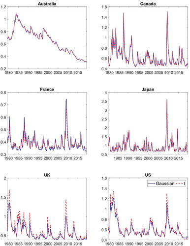
Figure A2. Probability integral transform – Australia.

Note: Vertical axes give relative frequency.

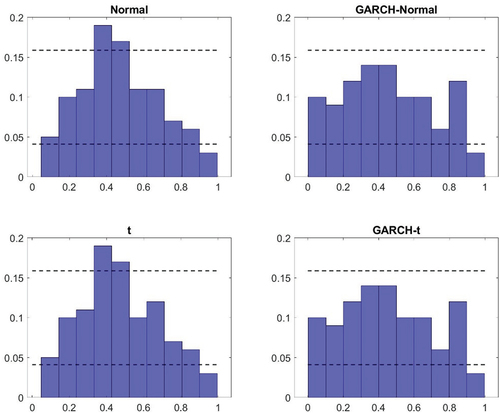
Figure A3. Probability integral transform – Canada.

Note: Vertical axes give relative frequency.

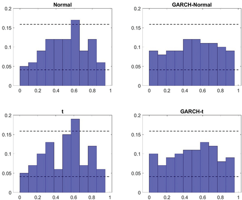
Figure A4. Probability integral transform – France.

Note: Vertical axes give relative frequency.

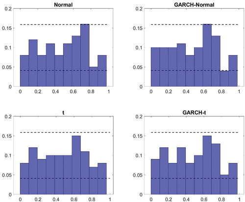
Figure A5. Probability integral transform – Japan.

Note: Vertical axes give relative frequency.

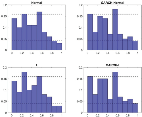
Figure A6. Probability integral transform – United Kingdom.

Note: Vertical axes give relative frequency.

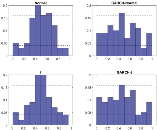
Figure A7. Probability integral transform – United States.

Note: Vertical axes give relative frequency

References

- Aastveit, K., K. Gerdrup, A. S. Jore, and L. A. Thorsrud. 2014. “Nowcasting GDP in Real-Time: A Density Combination Approach.” Journal of Business and Economic Statistics 32 (1): 48–68. doi:10.1080/07350015.2013.844155.
- Adrian, T., F. Grinberg, N. Liang, and S. Malik. 2018. “The Term Structure of Growth-At-Risk.” IMF Working Paper 18/180.
- Adrian, T., N. Boyarchenko, and D. Giannone. 2019. “Vulnerable Growth.” The American Economic Review 109 (4): 1263–1289. doi:10.1257/aer.20161923.
- Amisano, G., and R. Giacomini. 2007. “Comparing Density Forecasts via Weighted Likelihood Ratio Tests.” Journal of Business and Economic Statistics 25 (2): 177–190. doi:10.1198/073500106000000332.
- Anderson, T. W., and D. A. Darling. 1952. “Asymptotic Theory of Certain “Goodness of Fit” Criteria Based on Stochastic Processes.” Annals of Mathematical Statistics 23 (2): 193–212. doi:10.1214/aoms/1177729437.
- Anderson, T. W., and D. A. Darling. 1954. “A Test of Goodness of Fit.” Journal of the American Statistical Association 49 (268): 765–769. doi:10.1080/01621459.1954.10501232.
- Angelini, E., G. Camba‐mendez, D. Giannone, L. Reichlin, and G. Rünstler. 2011. “Short-Term Forecasts of Euro Area GDP Growth.” The Econometrics Journal 14 (1): C25–C44. doi:10.1111/j.1368-423X.2010.00328.x.
- Ascari, G., G. Fagiolo, and A. Roventini. 2015. “Fat-Tail Distributions and Business-Cycle Models.” Macroeconomic Dynamics 19 (2): 465–476. doi:10.1017/S1365100513000473.
- Banbura, M., D. Giannone, and L. Reichlin. 2011. “Nowcasting.” In The Oxford Handbook of Economic Forecasting, edited by M. P. Clements and D. F. Hendry, pp. 63–90. Oxford: Oxford University Press .
- Bao, Y., T.-H. Lee, and B. Saltoglu. 2007. “Comparing Density Forecast Models.” Journal of Forecasting 26 (3): 203–225. doi:10.1002/for.1023.
- Bollerslev, T. 1986. “Generalized Autoregressive Conditional Heteroskedasticity.” Journal of Econometrics 31 (3): 307–327. doi:10.1016/0304-4076(86)90063-1.
- Britton, E., P. Fisher, and J. Whitley. 1998. “The Inflation Report Projections: Understanding the Fan Chart“. Bank of England Quarterly Bulletin 1998, 30–37.
- Carriero, A., and T. E. Clark. 2015. “Realtime Nowcasting with a Bayesian Mixed Frequency Model with Stochastic Volatility.” Journal of the Royal Statistical Society: Series A (Statistics in Society) 178 (4): 837–862. doi:10.1111/rssa.12092.
- Cepni, O., I. E. Guney, and N. R. Swanson. 2020. “Forecasting and Nowcasting Emerging Market GDP Growth Rates: The Role of Latent Global Economic Policy Uncertainty and Macroeconomic Data Surprise Factors.” Journal of Forecasting 39 (1): 18–36. doi:10.1002/for.2602.
- Chauvet, M., and S. Potter 2013. “Forecasting Output” In Handbook of Economic Forecasting, edited by G. Elliott and A. Timmermann, Vol. 2, pp. 141–194. Amsterdam: Elsevier.
- Chiu, C. W. J., H. Mumtaz, and G. Pinter. 2017. “Forecasting with VAR Models: Fat Tails and Stochastic Volatility.” International Journal of Forecasting 33: 1124–1143.
- Christiano, L. J. 2007. “[On the Fit of New Keynesian Models]: Comment.” Journal of Business and Economic Statistics 25 (2): 143–151. doi:10.1198/073500107000000061.
- Chung, H., J.-P. Laforte, D. Reifschneider, and J. C. Williams. 2012. “Have We Underestimated the Likelihood and Severity of Zero Lower Bound Events?” Journal of Money, Credit, and Banking 44: 47–82. doi:10.1111/j.1538-4616.2011.00478.x.
- Clarida, R., J. Galí, and M. Gertler. 1998. “Monetary Policy Rules in Practice: Some International Evidence.” European Economic Review 42 (6): 1033–1067. doi:10.1016/S0014-2921(98)00016-6.
- Clark, T. E. 2011. “Real-Time Density Forecasts from Bvars with Stochastic Volatility.” Journal of Business and Economic Statistics 29 (3): 327–341. doi:10.1198/jbes.2010.09248.
- Clark, T. E., and F. Ravazzolo. 2015. “Macroeconomic Forecasting Performance Under Alternative Specifications of Time‐varying Volatility.” Journal of Applied Econometrics 30 (4): 551–575. doi:10.1002/jae.2379.
- Clements, M. P., and A. B. Galvão. 2013. “Real-Time Forecasting of Inflation and Output Growth with Autoregressive Models in the Presence of Data Revisions.” Journal of Applied Econometrics 28 (3): 458–477. doi:10.1002/jae.2274.
- Cogley, T., S. Morozov, and T. J. Sargent. 2005. “Bayesian Fan Charts for U.K. Inflation: Forecasting and Sources of Uncertainty in an Evolving Monetary System.” Journal of Economic Dynamics and Control 29 (11): 1893–1925. doi:10.1016/j.jedc.2005.06.005.
- Croushore, D., and T. Stark. 2001. “A Real-Time Data Set for Macroeconomists.” Journal of Econometrics 105 (1): 111–130. doi:10.1016/S0304-4076(01)00072-0.
- Diebold, F. X., and R. S. Mariano. 1995. “Comparing Predictive Accuracy.” Journal of Business and Economic Statistics 13: 253–263.
- Diebold, F. X., A. Gunther, and A. S. Tay. 1998. “Evaluating Density Forecasts with Application to Financial Risk Management.” International Economic Review 39 (4): 863–883. doi:10.2307/2527342.
- Diebold, F. X. 2015. “Comparing Predictive Accuracy, Twenty Years Later: A Personal Perspective on the Use and Abuse of Diebold–mariano Tests.” Journal of Business and Economic Statistics 33 (1): 1–9. doi:10.1080/07350015.2014.983236.
- Diks, C., V. Panchenko, and D. van Dijk. 2010. “Out-Of-Sample Comparison of Copula Specifications in Multivariate Density Forecasts.” Journal of Economic Dynamics & Control 34 (9): 1596–1609. doi:10.1016/j.jedc.2010.06.021.
- Engle, R. F. 1982. “Autoregressive Conditional Heteroscedasticity with Estimates of the Variance of United Kingdom Inflation.” Econometrica 50 (4): 987–1007. doi:10.2307/1912773.
- Fagiolo, G., M. Napoletano, and A. Roventini. 2008. “Are Output Growth-Rate Distributions Fat-Tailed?” Journal of Applied Econometrics 23 (5): 639–669. doi:10.1002/jae.1003.
- Faust, J., and J. H. Wright. 2009. “Comparing Greenbook and Reduced Form Forecasts Using a Large Realtime Dataset.” Journal of Business and Economic Statistics 27 (4): 468–479. doi:10.1198/jbes.2009.07214.
- Fountas, S., and M. Karanasos. 2007. “Inflation, Output Growth, and Nominal and Real Uncertainty: Empirical Evidence for the G7”.” Journal of International Money and Finance 26: 229–250.
- Giannone, D., L. Reichlin, and D. Small. 2008. “Nowcasting: The Real-Time Informational Content of Macroeconomic Data.” Journal of Monetary Economics 55 (4): 665–676. doi:10.1016/j.jmoneco.2008.05.010.
- Girardi, A., C. Gayer, and A. Reuter. 2016. “The Role of Survey Data in Nowcasting Euro Area GDP Growth.” Journal of Forecasting 35 (5): 400–418. doi:10.1002/for.2383.
- Hall, S. G., and J. Mitchell. 2007. “Combining Density Forecasts.” International Journal of Forecasting 23 (1): 1–13. doi:10.1016/j.ijforecast.2006.08.001.
- Hamilton, J. D. 2010. “Macroeconomics and ARCH.” In Volatility and Time Series Econometrics: Essays in Honor of Robert Engle, edited byM. Watson, T. Bollerslev, and J. Russell. Oxford:Oxford University Press.
- Hansen, P. R., and A. Lunde. 2005. “A Forecast Comparison of Volatility Models: Does Anything Beat a GARCH(1,1)?” Journal of Applied Econometrics 20 (7): 873–889. doi:10.1002/jae.800.
- Jansen, W. J., X. Jin, and J. M. de Winter. 2016. “Forecasting and Nowcasting Real GDP: Comparing Statistical Models and Subjective Forecasts.” International Journal of Forecasting 32 (2): 411–436. doi:10.1016/j.ijforecast.2015.05.008.
- Jarque, C. M., and A. K. Bera. 1980. “Efficient Tests for Normality, Homoscedasticity and Serial Independence of Regression Residuals.” Economics Letters 6 (3): 255–259. doi:10.1016/0165-1765(80)90024-5.
- Karlsson, S., and P. Österholm. 2020. “The Relation Between the Corporate Bond-Yield Spread and the Real Economy: Stable or Time-Varying?” Economics Letters 186: 108883. doi:10.1016/j.econlet.2019.108883.
- Kiss, T., and P. Österholm. 2020. “Fat Tails in Leading Indicators.” Economics Letters 193: 109317. doi:10.1016/j.econlet.2020.109317.
- Kiss, T., and P. Österholm. 2021. “Corona, Crisis and Conditional Heteroscedasticity.” Applied Economics Letters 28 (9): 755–759. doi:10.1080/13504851.2020.1776829.
- Kiss, T., S. Mazur, and H. Nguyen. 2022. “Predicting Returns and Dividend Growth — the Role of Non-Gaussian Innovations.” Finance Research Letters 46: 102315. doi:10.1016/j.frl.2021.102315.
- Kuzin, V., M. Marcellino, and C. Schumacher. 2011. “MIDAS vs. Mixed-Frequency VAR: Nowcasting GDP in the Euro Area.” International Journal of Forecasting 27: 529–542. doi:10.1016/j.ijforecast.2010.02.006.
- Liu, X. 2019. “On Tail Fatness of Macroeconomic Dynamics.” Journal of Macroeconomics 62: 103154. doi:10.1016/j.jmacro.2019.103154.
- Ljung, G. M., and G. E. Box. 1978. “On a Measure of Lack of Fit in Time Series Models.” Biometrika 65 (2): 297–303. doi:10.1093/biomet/65.2.297.
- Madhou, A., T. Sewak, I. Moosa, and V. Ramiah. 2017. “GDP Nowcasting: Application and Constraints in a Small Open Developing Economy.” Applied Economics 49 (38): 3880–3890. doi:10.1080/00036846.2016.1270417.
- Massey Jr, F. J. 1951. “The Kolmogorov-Smirnov Test for Goodness of Fit.” Journal of the American Statistical Association 46 (253): 68–78. doi:10.1080/01621459.1951.10500769.
- Mazzi, G. L., J. Mitchell, and G. Montana. 2014. “Density Nowcasts and Model Combination: Nowcasting Euro‐area GDP Growth Over the 2008–09 Recession.” Oxford Bulletin of Economics and Statistics 76 (2): 233–256. doi:10.1111/obes.12015.
- Mishkin, F. S. 2011. “Monetary Policy Strategy: Lessons from the Crisis.” NBER Working Paper 16755.
- Mitchell, J., and S. G. Hall. 2005. “Evaluating, Comparing and Combining Density Forecasts Using KLIC with an Application to the Bank of England and NIESR “Fan” Charts of Inflation.” Oxford Bulletin of Economics and Statistics 67 (s1): 995–1033. doi:10.1111/j.1468-0084.2005.00149.x.
- Mitchell, J., and K. F. Wallis. 2011. “Evaluating Density Forecasts: Forecast Combinations, Model Mixtures, Calibration and Sharpness.” Journal of Applied Econometrics 26 (6): 1023–1040. doi:10.1002/jae.1192.
- Mitchell, J., and M. Weale 2019. “Forecasting with Unknown Unknowns: Censoring and Fat Tails on the Bank of England’s Monetary Policy Committee.” EMF Research Papers 27.
- Pesaran, M. H., T. Schuermann, and L. V. Smith. 2009. “Forecasting Economic and Financial Variables with Global Vars.” International Journal of Forecasting 25 (4): 642–675. doi:10.1016/j.ijforecast.2009.08.007.
- Pontines, V. 2010. “Fat-Tails and House Prices in OECD Countries.” Applied Economics Letters 17 (14): 1373–1377. doi:10.1080/13504850902967514.
- Prasad, M. A., S. Elekdag, M. P. Jeasakul, R. Lafarguette, M. A. Alter, A. X. Feng, and C. Wang 2019. “Growth at Risk: Concept and Application in IMF Country Surveillance.” IMF Working Paper 19/36.
- Robertson, J. C., E. W. Tallman, and C. H. Whiteman. 2005. “Forecasting Using Relative Entropy.” Journal of Money, Credit, and Banking 37 (3): 383–401. doi:10.1353/mcb.2005.0034.
- Stock, J. H., and M. Watson. 2003. “Forecasting Output and Inflation: The Role of Asset Prices.” Journal of Economic Literature 41 (3): 788–829. doi:10.1257/jel.41.3.788.
- Trypsteen, S. 2017. “The Importance of Time‐varying Volatility and Country Interactions in Forecasting Economic Activity.” Journal of Forecasting 36 (6): 615–628. doi:10.1002/for.2457.