Diversification and hedging strategies of green bonds in financial asset portfolios during the COVID-19 pandemic

ABSTRACT

In this paper, we investigate whether investors can reap potential diversification or hedging benefits from holding green bonds in a portfolio containing a conventional financial asset during the COVID-19 pandemic. Using data from 6 November 2014 to 5 November 2020, we estimate corrected dynamic conditional correlation between between green bonds and four major asset classes: stocks, corporate bonds, commodities, and clean energy. We extend our analysis by using these correlations to examine hedging, optimal portfolio weights, and naïve strategies and evaluate their implications for investors by calculating hedging effectiveness and utility gain improvement. Results reveal that across the full sample, pre-COVID-19, and during-COVID-19 periods, optimal portfolio weights represent an ideal strategy to realize the greatest risk reduction and risk-adjusted return. Further, green bonds could add substantial diversification benefits for investors holding assets in clean energy, global stocks, and commodities.

KEYWORDS:

• Financial assets
• portfolio
• hedge
• diversification
• COVID-19

JEL CLASSIFICATION:

• G10
• G11
• G15

I. Introduction

Green bonds are novel fixed-income securities that are similar to corporate and treasury bonds but designed to finance projects with environmental benefits consistent with a climate-resilient economy (Reboredo 2018). Green bonds have recently received growing attention from environmentally conscious and traditional investors who acknowledge these assets’ possible financial benefits (Nguyen et al. 2020). Both types of investors began moving their funds to green bonds after the International Capital Markets Association published the ‘Green Bond Principles’ in 2014, guiding the issuance of these new securities. This regulatory step rendered green bonds more appealing to investors as a financial instrument in stock markets worldwide. These principles also motivated investors to begin using green bonds for hedging risk or portfolio diversification (Reboredo, Ugolini, and Aiube 2020). The size of the green bonds market has hence continued to expand, making these bonds a sustainable investment (Febi et al. 2018; Reboredo and Ugolini 2020).

Despite the increasing importance of green bonds, little is known about their role in portfolio management. Few studies have examined relationships between green bonds and conventional financial assets (Hammoudeh, Ajmi, and Mokni 2020). For instance, Reboredo (2018) investigated co-movement between the green bond and financial markets; results showed that green bonds offered negligible diversification benefits for investors in corporate and treasury markets, whereas diversification benefits were notable in the stock and energy markets. Reboredo and Ugolini (2020) and Reboredo, Ugolini, and Aiube (2020) examined price connectedness between the green bond and financial markets and revealed the green bond market to be weakly tied to the stock, energy, and high-yield corporate bond markets. Nguyen et al. (2020) confirmed these outcomes, indicating that green bonds generated diversification benefits due to their low negative correlations with stocks and commodities. Finally, Jin et al. (2020) explored the hedging effect of green bonds on carbon market risk and noted that these bonds represent an effective hedger for carbon futures.

Our study extends relevant literature by assessing whether potential diversification/hedging benefits come from holding green bonds in a portfolio constructed for a conventional financial asset during COVID-19¹ We investigated this topic using a five-variable system, including stock, corporate bond, commodity, clean energy, and green bond price series from 6 November 2014 to 5 November 2020. Specifically, we employed Aielli’s (2013) corrected dynamic conditional correlation-GARCH (cDCC-GARCH) model, which corrects for inconsistent estimation of the correlation matrix in Engle’s (2002) DCC model. Based on the cDCC model, we estimated dynamic co-movements between green bonds and financial assets and derived hedge ratios, optimal portfolio weights, hedging effectiveness, and utility gains for different portfolio strategies (i.e. diversified portfolios and hedged portfolios).

Our empirical results revealed that green bonds could be an integral part of a diversified portfolio of conventional financial assets over the full sample period in addition to the pre- and during-COVID-19 sub-periods. Further, investors should favour an optimal portfolio weight strategy, which achieved the best risk/downside risk reduction and utility gain improvement versus the optimal hedge ratio and naïve strategies. Finally, investors should allocate, on average, the largest portion of their funds to green bonds when constructing most financial asset portfolios. Green bonds offer sizable diversification benefits for investors in clean energy, global stocks, and commodities.

This study’s contributions to the literature are threefold. First, we examined how the dynamics between green bonds and an array of conventional financial assets changed before and during COVID-19. We chose COVID-19 as a study period given the unique nature of the joint health and economic crises resulting from the pandemic and its adverse effects on most stock markets around the world. The economic impact of the spread of COVID-19 has heightened market risk aversion in ways unseen since the global financial crisis, leading stock markets to decline by more than 30% (OECD 2020; Zhang, Hu, and Ji 2020; Gupta et al. 2021). These challenges provide a novel research setting to examine whether green bonds can protect investors during this time of unprecedented uncertainty. Second, we illustrated period-specific implications of green bond – financial asset dynamics on portfolio management strategies by analysing hedging ratios, optimal portfolio weights, and downside hedging effectiveness. Findings provide useful insight to investors about how each portfolio strategy performed across sub-periods to identify the preferred portfolio allocation. Third, for each sub-study period, we considered economic implications from green bond hedging. In particular, we calculated utility gains available to investors upon hedging each financial asset with green bonds, which are based on risk-adjusted performance (Maitra, Chandra, and Dash 2020).

The rest of this paper is organized as follows. Section II provides a description of the data. Section III discusses our methodology. Section IV presents empirical findings, and Section V concludes our work.

II. Data and descriptive analysis

Data

Our dataset consisted of daily prices for green bonds plus four conventional financial assets (i.e. stocks, corporate bonds, commodities, and clean energy), respectively represented as follows: the MSCI world index (WORLD), PIMCO Investment-Grade Corporate Bonds Index (PIMCO), Bloomberg Commodity Index (COMM), and S&P Global Clean Energy Index (CLEAN). All price series were considered from 6 November 2014 to 5 November 2020. For our purposes, green bond (financial asset) returns were defined as the difference in the logarithms of two consecutive prices of a given price index: $r_{it}=log\left(p_{it}/p_{it}-1\right)\times 100$. All price series were extracted from the Refinitiv database.

Based on recent studies (e.g. Akhtaruzzaman, Boubaker, and Sensoy 2021; Sakurai and Kurosaki 2020; Salisu, Vo, and Lawal 2020), the first case of COVID-19 was announced in China on 31 December 2019. The virus was deemed an epidemic with normal levels of apparent risk until 19 February 2020; the following day, COVID-19 was named a worldwide threat. Investors’ uncertainty caused global stock markets to plummet. Therefore, to examine whether the COVID-19 pandemic influenced co-movements or hedging and diversification strategies between green bonds and other financial assets, we split our sample into two sub-periods: Sub-period 1 (pre-COVID-19), covering 6 November 2014–19 February 2020; and Sub-period 2 (during COVID-19), covering 20 February 2020–5 November 2020.

Descriptive analysis

Table 1 presents descriptive statistics for the daily return series of green bonds and four conventional financial assets over the full study period.

Table 1. Descriptive Statistics of the returns.

	GREEN	WORLD	PIMCO	COMM	CLEAN
Mean	0.009	0.024	0.008	−0.026	0.047
Median	0.007	0.052	0.009	0.001	0.072
SD	0.318	0.983	0.434	0.840	1.370
Minimum	−2.410	−10.441	−5.083	−4.268	−12.498
Maximum	2.013	8.406	6.818	3.390	11.035
Skewness	−0.579	−1.510	−0.010	−0.357	−1.049
Kurtosis-3	6.326	23.809	74.710	2.4642	15.546
JB	2697.3**	37560**	363970**	429.17**	16046**
Q(20)	20.390	194.776**	21.227	18.1201	30.795*
Q^2(20)	580.030**	1923.74**	1424.340**	485.628**	1723.22**
ADF	−15.990**	−17.508**	−13.7965**	−16.466**	−16.374**
KPSS	0.048	0.026	0.089	0.192	0.499
ARCH(10)	34.247**	89.292**	83.978**	19.707**	70.772
Corr. with Green	1.000	0.127	0.378	0.180	0.159

The reported statistics are for daily returns of green bond and conventional financial assets (MSCI world, Pimco bonds, Commodity, and Clean energy) indices for the period from 6 November 2014 to 5 November 2020. SD is the standard deviation. JB denotes the Jarque- Bera test for normality. Q(20) and Q² (20) are Box-Pierce statistics for serial correlation in return and square returns up to 20 lags. ADF is the augmented Dicky-Fuller unit root test, while KPSS is the Kwiatkowski-Phillips-Schmidt-shin test for stationarity. ARCH (10) is the heteroscedasticity test of Engle (1982) up to 20 lags. Corre. With Green is the constant correlation between green bond and each of conventional financial assets. **, * indicate statistical significance at 1% and 5% levels, respectively.

We observed that the average return of CLEAN and its volatility (measured by standard deviation) was highest among all sampled assets, exhibiting higher risk – higher return features. All return distributions showed negative skewness and were leptokurtic with higher peaks and fat tails; thus, the return series were not normally distributed as evidenced by the Jarque – Bera test. Box – Pierce test statistics (calculated up to 20 lags) led us to reject the null hypothesis of no autocorrelation in two return series (WORLD and CLEAN). However, the non-linear version of this test indicated that all squared return series were subject to autocorrelation. We also noted that all return series were stationary, as confirmed by the augmented Dickey – Fuller and Kwiatkowski – Phillips–Schmidt – Shin tests. Engle’s (1982) ARCH LM test with 10 lags supported the existence of heteroscedasticity in all return series. Therefore, using the cDCC-GARCH model might be suitable to capture the time-varying return volatility. Finally, the relatively low values of constant correlations for most return series reflected the diversification potential of portfolios containing green bonds and other conventional financial assets (see Wen, Bouri, and Roubaud 2017).

III. Methodology

In this section, we discuss our simplified approach to model DCCs between daily green bonds and financial assets (i.e. stocks, corporate bonds, commodities, and clean energy). We adopted Aielli’s (2013) cDCC-GARCH model, which corrects for inconsistent estimation of the correlation matrix in Engle’s (2002) DCC approach. The cDCC model can capture dynamic co-movements between securities and is hence used to explore hedging and diversification benefits among asset categories (Ghabri, Guesmi, and Zantour 2020). cDCC estimation consists of two steps (Shahzad et al. 2017): (1) univariate GARCH models are estimated for each return series, and (2) the conditional correlation dynamics are computed.

Under the cDCC process, the AR (1) multivariate return is formulated as follows:

(1) $r_t=\mu +\delta r_{t-1}+{\epsilon }_{it},where{\epsilon }_t=z_t\sqrt{H_t}$(1)

where $r_t$ is an $N\times 1$ vector of returns of green bonds or a conventional financial asset (stocks, corporate bonds, commodities, or clean energy); µ is the vector of $N\times 1$ conditional mean $\mu =E\left(r_t{I}_t-1\right)$ is the $N\times 1$ corresponding vector of autoregressive returns of order 1; and $\delta$ is an $N\times 1$ vector of the parameters of autoregressive returns. ε_t is an $N\times 1$ vector of residuals. z_t is an $N\times 1$ vector of standardized residuals, which follow the Student’s t distribution with v degrees of freedom. H_t is an $N\times N$ time-varying variance – covariance matrix of r_t. Next, the conditional variance h_t is obtained from the univariate GARCH (1, 1) model:

(2) $h_t=\omega +\alpha {\epsilon }_{t-1}^2+b{h}_{it-1}^2$(2)

where h_t is the conditional variance of the return series; ω is a constant that measures unconditional volatility; α captures the ARCH effect reflecting short-term persistence; and b captures the GARCH effect reflecting long-term persistence (Abuzayed, Al-Fayoumi, and Bouri 2020).

In the next step, the correlation matrix is estimated from the standardized residuals of the GARCH (1,1) model for green bonds and each of the financial asset returns. Assume that the variance – covariance matrix can be decomposed as H_t = D_t R_t D_t, where R_t is the time-varying correlation matrix and D_t = diag √h_t is a diagonal matrix of standard deviations from the univariate GARCH (1,1) model (Maitra, Chandra, and Dash 2020). Under the DCC process, R_t depicts the dynamic correlation structure as follows (Sensoy, Hacihasanoglu, and Nguyen 2015): $R_t=[diag{(Q_t)}^{-1/2}{Q}_t[diag{(Q_t)}^{-1/2}$. Here, $Q_t=\left(1-{\theta }_1-{\theta }_2\right)Q^{\prime }+\hspace{0.17em}{\theta }_1\left({\mathrm{z}}_{t-1}{{\mathrm{z}}^{\prime }}_{t-1}\right)+{\theta }_2{Q}_{t-1}$ Unexpected text node ‘z’. Specifically, Q’ is the unconditional covariance matrix of standardized residuals z_t. The parameters ${\theta }_1$and ${\theta }_2$ are non-negative scalar coefficients with a sum of less than unity. Aielli’s (2013) stated that the DCC process incorporates a significant asymptotic bias in the estimator of the covariance matrix; as such, the correlation evolution process is

(3) $Q_t=\left(1-{\theta }_1-{\theta }_2\right)Q{ }^{\mathrm{\prime }}+\hspace{0.17em}{\theta }_1\{diag(Q_{t-1}{)}^{\frac{1}{2}}\left({\mathrm{z}}_{t-1}{\mathrm{z}{ }^{\mathrm{\prime }}}_{t-1}\right)diag(Q_{t-1}{)}^{-\frac{1}{2}}\}+{\theta }_2{Q}_{t-1}$(3)

Finally, the time-varying correlation (${\rho }_{gi,t})$ between green bonds (g) and a financial asset (i) at time t is defined as

(4) ${\rho }_{gi,t}=\frac{q_{gi,t}}{\sqrt{q_{gg}}\sqrt{q_{ii}}}$(4)

We used quasi-maximum likelihood estimation to estimate the multivariate cDCC-GARCH (1, 1) model.

IV. Empirical results

Dynamic conditional correlation analysis

In this sub-section, we examine the time-varying co-movement between each financial asset return and green bonds based on the multivariate cDCC-GARCH model described in Section III. Findings appear in Table 2.

Table 2. Parameter estimates for cDCC model based on multivariate Student distribution.

	GREEN	WORLD	PIMCO	COMM	CLEAN
Panel A: Mean equation
μ	0.013** (0.007)	0.069** (0.017)	0.012 (0.006)	−0.011 (0.018)	0.0508 (0.028)
δ	0.017 (0.027)	0.073* (0.031)	−0.037 (0.028)	−0.033 (0.027)	0.164** (0.028)
Panel B: Variance equation
ω	0.002 (0.001)	0.024** (0.007)	0.007** (0.002)	0.0135* (0.006)	0.031* (0.013)
α	0.071** (0.023)	0.240** (0.049)	0.138** (0.031)	0.051** (0.011)	0.127** (0.032)
b	0.914** (0.026)	0.751** (0.038)	0.781** (0.048)	0.929** (0.016)	0.858** (0.033)
Panel C: DCC equation
θ1	0.021** (0004)
θ2	0.942** (0.013)
v	7.235** (0.501)
Panel D: Diagnostic tests
BP Q(20)	30.1925 [0.067}	23.0515 [0.286]	26.291 [0.156]	15.376 [0.754]	11.345 [0.936]
BP Q^2(20)	25.014 [0.201]	16.610 [0.678]	30.772 [0.0582]	12.411 [0.901]	16.479 [0.686]

Panels A B, and C show the estimated coefficients of the conditional mean, conditional variance and conditional correlation for all full-period from 6 November 2014 to 5 November 2020. Panel D presents the diagnostic tests. ρ_ig is the expected value of the dynamic conditional correlations between financial assets and green bond, while θ₁ and θ₂ examine the influences of last period’s residuals and covariance on the current level of the covariance. v is student’s t distribution shape parameter. The Panel D reports diagnostic test statistics for the univariate and multivariate standardized residuals for the cDCC- GARCH(1,1) model. BP-Q (20) and BP²-Q (20) stand for the Box – Pierce-Q statistics for standardized and standardized squared residuals, respectively, for up to 20 lags. Robust standard errors of the estimated coefficients are given in parenthesis and the p-values of the diagnostic tests are given in square brackets. ** and * denote statistical significance at the 1% and 5% significance levels, respectively.

Panel A presents results of the conditional mean equation for each index; it shows that the one-lag return of the WORLD and CLEAN indices was positive and significant, whereas the other indices showed no significance in the lagged return. Panel B lists the results of the conditional variance equation. All return-index lagged shock squared (α) and lagged volatility values (b) were positive and highly significant at the 1% level, implying that past shocks and volatility enhanced current volatility. As the estimation of b exceeded that of α for each return index, the returns appeared more sensitive to past volatility than to past shocks (Jin et al. 2020). Panel C contains the estimate of the multivariate cDCC process. The parameters θ₁ and θ₂ were each highly significant at the 1% level, suggesting that the cDCC model captured time-varying correlations between green bond and financial asset indices. The significant estimated values of the Student’s t distribution shape parameter v suggested that the residual terms in Equation. (1)(1) $r_t=\mu +\delta r_{t-1}+{\epsilon }_{it},where{\epsilon }_t=z_t\sqrt{H_t}$(1) were not normal, consistent with descriptive statistics in Table 1. The diagnostic tests reported in Panel D supported the accurate specification of our cDCC-GARCH (1,1) model, as the Box – Pierce Q-test statistics for standardized and standardized squares did not reject the null hypothesis of no serial correlation for all indices.

The results in Table 2 only show estimates of the cDCC model over the full sample period; Table 3 (Panel A) displays the descriptive statistics for correlations between green bonds and each financial asset during the full period and each sub-period before and after the COVID-19 pandemic. Their time-varying movements are plotted in Figure 1.

Figure 1. Dynamic conditional correlations.

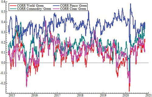
Table 3. DCC, Hedge ratios and optimal portfolio weights summary statistics.

	Full sample					Pre-COVID-19				During COVID-19
	Mean	SD	Min	Max		Mean	SD	Min	Max	Mean	SD	Min	Max
Panel A: DCC
WORLD/GREEN	0.088	0.099	−0.281	0.410		0.086	0.099	−0.224	0.410	0.103	0.099	−0.281	0.235
PIMCO/GREEN	0.367	0.066	0.140	0.581		0.368	0.064	0.140	0.539	0.364	0.076	0.197	0.581
COMM/GREEN	0.177	0.080	0.156	0.409		0.172	0.078	−0.121	0.409	0.208	0.087	−0.156	0.361
CLEAN/GREEN	0.117	0.089	−0.238	0.415		0.115	0.088	−0.238	0.415	0.131	0.095	−0.200	0.253
Panel B: HR
WORLD/GREEN	0.205	0.354	−2.397		2.864	0.193	0.310	−1.143	2.864	0.292	0.576	−2.397	1.389
PIMCO/GREEN	0.369	0.156	0.142		1.964	0.355	0.107	0.142	0.815	0.474	0.330	0.178	1.963
COMM/GREEN	0.485	0.231	−0.221		1.228	0.476	0.225	−0.316	1.228	0.551	0.263	−0.521	1.132
CLEAN/GREEN	0.436	0.431	−2.104		2.341	0.398	0.365	−1.006	2.341	0.724	0.693	−2.105	2.127
Panel C: Portfolio weights
WORLD/GREEN	0.843	0.111	0.428		1.000	0.830	0.110	0.428	1.000	0.938	0.053	0.732	1.000
PIMCO/GREEN	0.472	0.164	0.060		1.000	0.456	0.153	0.060	0.898	0.584	0.194	0.238	1.000
COMM/GREEN	0.923	0.047	0.725		1.000	0.922	0.048	0.725	1.000	0.932	0.041	0.815	1.000
CLEAN/GREEN	0.945	0.048	0.712		1.000	0.939	0.047	0.712	1.000	0.990	0.011	0.878	1.000

The table shows summary statistics of dynamic conditional correlations, hedge ratios, and optimal weights for the portfolios between each conventional asset and green bond. We report the results for the full period and each sub-sample period (pre- and during COVID-19).

In Panel A of Table 3, for the full period, the WORLD – GREEN, COMM – GREEN, and CLEAN – GREEN pairs presented the lowest average conditional correlation (0.09, 0.18, and 0.12, respectively). By contrast, the PIMCO – GREEN pair demonstrated the highest average conditional correlation (0.37). As such, although green bonds may exhibit strong potential for diversifying WORLD, COMM, and CLEAN risks, these bonds may provide a better hedging opportunity for PIMCO. In each sub-period, all average conditional correlations displayed nearly similar trends to the full period. Figure 1 confirms these results. Time-varying correlations were low for all financial assets throughout the sample period; the exception is PIMCO, whose correlation was much higher than the others.

Optimal hedging ratio and weight analysis

In this sub-section, we examine whether investors may hedge financial asset risk exposure using green bonds. Based on conditional variance and covariance estimates from the cDCC-GARCH model, we calculated hedge ratios and portfolio weights to construct alternative portfolio strategies.

First, we computed the optimal hedging ratio reflecting the amount of short positions (sell) in green bonds (β_t) that minimizes the risk of a long position (buy) in the financial asset. Following Kroner and Sultan (1993) and Abuzayed, Al-Fayoumi, and Bouri (2020), we calculated the optimal hedge ratio as

(5) ${\beta }_t=\frac{h_{ig,t}}{h_{gg,t}}$(5)

where ${\beta }_t$ is the time-varying hedging ratio at time t, $h_{ig,t}$ is the conditional covariance between financial asset and green bond returns at time t, and $h_{gg,t}$ is the conditional variance of green bond returns at time t.

Summary statistics of the time-varying hedging ratio for each of the four financial assets and green bonds are displayed in Panel B of Table 3. Their time-varying movements appear in Figure 2.

Figure 2. Optimal hedge ratios.

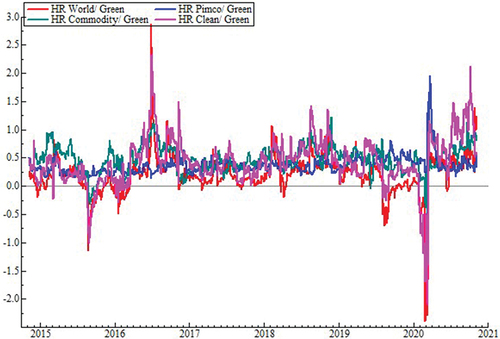
COMM had the highest hedge ratio during the full sample period (0.48), followed by CLEAN (44%) and PIMCO (37%); the hedge ratio of WORLD was lowest (0.21). We found that green bonds were the least useful (i.e. the most expensive hedge) against the volatility of commodities but represented the cheapest hedge for the WORLD index. For instance, the $1 long position in COMM could be hedged for 48 cents with a short position in GREEN. Comparatively, the $1 long position in WORLD could be hedged for 21 cents with a short position in GREEN. Regarding period-wise average hedging ratios in Panel B, all financial asset hedging ratios and their associated standard deviations increased noticeably during COVID-19 relative to before. Figure 2 verifies this result, such that pairwise hedging ratios were time-varying and showed considerable volatility during the COVID-19 period. This pattern implies that a relatively heavy short position in green bonds would be required to hedge risk exposure in financial assets, while higher hedging costs would be needed when applying dynamic hedging strategies for portfolio management (Jin et al. 2020).

Second, given that investors seek to minimize portfolio risk for a given expected return, the optimal portfolio weight can be determined to realize this goal (Kroner and Ng 1998; Zhang, Hu, and Ji 2020). In our study, the optimal weight of green bonds (w_g,t) in a portfolio of each financial asset i and green bond g is given by

$w_{g,t}=\frac{h_{ii,t}-h_{ig,t}}{h_{gg,t}-2h_{ig,t}+h_{ii,t}}$

And

(6) $w_{g,t}=\left\{\begin{array}{c}0if{w}_{g,t}<0\\ w_{g,t}if0\le w_{g,t}\le 1\\ 1if{w}_{g,t}>1\end{array}\right.$(6)

Accordingly, the weight to be invested in financial asset i is denoted as $\left(1-w_{g,t}\right).$

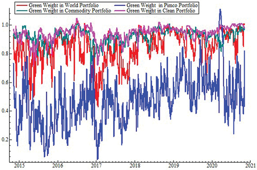
Panel C of Table 3 lists descriptive statistics of optimal weights for a two-asset portfolio comprising green bonds and one type of financial asset. During the full sample period, green bonds had the highest weight in the CLEAN – GREEN portfolio (0.94) followed by COMM – GREEN (0.92) and WORLD – GREEN (0.84); these bonds had the lowest weight in PIMCO – GREEN (0.47). Accordingly, the average weight for the CLEAN – GREEN portfolio indicated that of a $1 portfolio, 94 cents should be invested in green bonds and 0.06 in clean energy stocks. The average weight for PIMCO – GREEN suggests that out of $1, 47 cents should go to a green bonds index and 53 cents to PIMCO bonds. Portfolio risk can thus be minimized without reducing the expected return if investors assign a higher weight to green bonds than financial assets in all portfolios (except PIMCO – GREEN).

Table 3 also contains the descriptive statistics of period-wise optimal portfolio weights. For instance, before the COVID-19 period, results were similar to the entire sampling period as investors held more green bonds than financial assets aside from PIMCO. The average values of green bond weights in financial asset portfolios equalled 0.83, 0.46, 0.92, and 0.94 in WORLD, PIMCO, COMM, and CLEAN, respectively. During the COVID-19 period, investors appeared to follow a similar portfolio diversification strategy that allocated more weight to green bonds compared with the pre-COVID-19 period: average values of green bond weights were 0.94, 0.58, 0.93, and 0.99 in WORLD, PIMCO, COMM, and CLEAN, respectively.

Moreover, these weights exhibited a time-varying characteristic (see Figure 3). We identified no sizable variations in their behaviour (except PIMCO – GREEN), and their standard deviations were relatively low on average and declined during the COVID-19 period. This finding implies that green bonds demonstrated stable weights with all financial assets (except with PIMCO) and consequently did not require frequent portfolio rebalancing during diversification, which can be expensive (Olson, Vivian, and Wohar 2017; Junttila, Pesonen, and Raatikainen 2018; Belhassine 2020).

Figure 3. Optimal green bond weights.

Portfolio performance measures

We also investigated whether green bonds should be chosen to diversify the risk exposure of conventional financial assets during the full sample period and before and after the COVID-19 pandemic. Following Wen, Bouri, and Roubaud (2017), Ahmad and Rais (2018), and Kang and Yoon (2020), we constructed three portfolios to compare with a benchmark portfolio (Portfolio I) composed of one financial asset: a hedge ratio (variance-minimizing) portfolio (Portfolio II), an optimal weight portfolio (Portfolio III), and a naïve (equally weighted) portfolio (Portfolio IV). We assessed each portfolio’s volatility, downside risk, and utility gain for investors, which are related to risk-adjusted performance (Maitra, Chandra, and Dash 2020).

The variance reduction effectiveness of each financial asset with green bonds is written as

(7) $H{E}_j=\left[\frac{va{r}_{unhedge-}va{r}_{hedged}}{va{r}_{unhedged}}\right]$(7)

where HE is the hedging effectiveness; var_unhedged is the variance of an unhedged return for one of the four financial assets (benchmark Portfolio I), estimated from the cDCC model; and var_hedged denotes the variance of hedged portfolio j’s (j= II, III,IV) return. A higher HE_j value indicates greater risk reduction. We also examined each portfolio’s downside (extreme) risk effectiveness based on value at risk (VaR) and expected shortfall (ES) and evaluated the economic implications of portfolio hedging based on utility gain.

When the portfolio return follows a Student’s t distribution with the $t_v^{-1}$(p^th) quantile and v degrees of freedom and a 95% confidence level, VaR is given as (see Rehman, Asghar, and King 2020):

(8) $Va{R}_{j,t}\left(5\mathrm{\%}\right)=-{\mu }_{j,t}-{\sigma }_{j,t}{t}_v^{-1}$(8)

where µ and σ are the conditional mean and standard deviation of portfolio j; and

The ES is expressed as:

(9) $E{S}_{j,t}\left(5\mathrm{\%}\right)=-{\mu }_{j,t}+\frac{{\sigma }_{jt}}{p}\mathrm{\varnothing }\left(t_v^{-1}\left(p\right)\right)\left[\frac{v+t_v^{-1}\left(p^2\right)}{v-1}\right],$(9)

where $\mathrm{\varnothing }$ is a cumulative density function.

Finally, The expected utility (EU) for portfolio j can be calculated as:

(10) $E{U}_{j,t}\mid I_{t-1}=E\left(r_{j,t}|I_{t-1}\right)-\gamma Var\left(r_{j,t}|I_{t-1}\right),$(10)

where$\hspace{0.17em}{r}_{j,t}$ is the return of portfolio j; $\gamma$_t is the level of investor’s risk aversion, which is assumed to equal 4; and Var is the variance of the portfolio return (see Batten et al. 2021; Maitra, Chandra, and Dash 2020).

Table 4 reports the average risk/downside risk reduction and utility gain improvement of portfolios consisting of green bonds and each financial asset compared with the benchmark portfolio (Portfolio I).

Table 4. Portfolios’ average risk/downside risk reduction and utility gain improvement.

Portfolio	Portf. I	Portf. II	Portf. III	Portf IV	Portf. II	Portf. III		Portf. IV
Panel A	Variance				Hedging Effectiveness
Full period
WORLD/GREEN	1.037	1.018	0.088	0.296	0.018	0.915	0.714
PIMCO/GREEN	0.152	0.121	0.066	0.086	0.204	0.566	0.434
COMM/GREEN	0.695	0.668	0.096	0.222	0.039	0.862	0.681
CLEAN/GREEN	1.892	1.850	0.098	0.521	0.022	0.948	0.724
Pre-Covid-19
WORLD/GREEN	0.563	0.550	0.073	0.170	0.023	0.870	0.696
PIMCO/GREEN	0.075	0.064	0.052	0.056	0.147	0.307	0.253
COMM/GREEN	0.644	0.610	0.084	0.201	0.053	0.870	0.688
CLEAN/GREEN	1.121	1.096	0.085	0.318	0.022	0.924	0.716
During Covid-19
WORLD/GREEN	4.550	4.485	0.190	1.223	0.014	0.958	0.973
PIMCO/GREEN	0.723	0.542	0.165	0.309	0.250	0.772	0.573
COMM/GREEN	1.149	1.100	0.184	0.381	0.043	0.840	0.654
CLEAN/GREEN	7.603	7.440	0.195	2.024	0.021	0.974	0.973
Panel B	Value-at-risk (VaR)				VaR reduction
Full period
WORLD/GREEN	1.292	1.286	0.417	0.742	0.005	0.677	0.426
PIMCO/GREEN	0.509	0.457	0.394	0.404	0.102	0.226	0.206
COMM/GREEN	1.375	1.354	0.476	0.777	0.015	0.654	0.435
CLEAN/GREEN	1.899	1.818	0.464	0.954	0.043	0.745	0.498
Pre-Covid-19
WORLD/GREEN	1.090	1.078	0.393	0.638	0.011	0.639	0.415
PIMCO/GREEN	0.449	0.402	0.372	0.371	0.105	0.171	0.174
COMM/GREEN	1.325	1.308	0.454	0.746	0.013	0.657	0.437
CLEAN/GREEN	1.640	1.563	0.442	0.831	0.047	0.730	0.493
During Covid-19
WORLD/GREEN	2.790	2.828	0.594	1.514	−0.014	0.787	0.457
PIMCO/GREEN	0.955	0.867	0.549	0.647	0.092	0.425	0.322
COMM/GREEN	1.741	1.699	0.637	1.007	0.024	0.634	0.421
CLEAN/GREEN	3.823	3.709	0.627	1.871	0.030	0.836	0.511
Portfolio	Portf. I	Portf. II	Portf. III	Portf IV	Portf. II	Portf. III	Portf IV
Panel C	Expected Shortfall (ES)				ES reduction
Full period
WORLD/GREEN	1.594	1.581	0.564	0.887	0.008	0.646	0.444
PIMCO/GREEN	0.610	0.568	0.479	0.507	0.069	0.215	0.169
COMM/GREEN	1.669	1.641	0.597	0.941	0.017	0.642	0.436
CLEAN/GREEN	2.365	2.344	0.598	1.258	0.001	0.747	0.468
Pre-Covid-19
WORLD/GREEN	1.354	1.344	0.533	0.767	0.007	0.606	0.434
PIMCO/GREEN	0.536	0.502	0.449	0.463	0.063	0.162	0.136
COMM/GREEN	1.611	1.586	0.571	0.907	0.016	0.646	0.437
CLEAN/GREEN	2.031	2.013	0.570	1.090	0.009	0.719	0.463
During Covid-19
WORLD/GREEN	3.372	3.345	0.789	1.779	0.008	0.766	0.472
PIMCO/GREEN	1.162	1.050	0.703	0.836	0.096	0.395	0.281
COMM/GREEN	2.095	2.049	0.789	1.198	0.022	0.623	0.428
CLEAN/GREEN	4.844	4.497	0.804	2.505	0.072	0.834	0.483
Panel D	Utility				Utility improvement
Full period
WORLD/GREEN	−4.125	−4.074	−0.342	−1.169	0.012	0.917	0.717
PIMCO/GREEN	−0.600	−0.488	−0.255	−0.336	0.187	0.477	0.440
COMM/GREEN	−2.806	−2.708	−0.378	−0.898	0.035	0.865	0.680
CLEAN/GREEN	−7.519	−7.360	−0.383	−2.057	0.021	0.949	0.726
Pre-Covid-19
WORLD/GREEN	−2.228	−2.178	−0.291	−0.670	0.022	0.869	0.699
PIMCO/GREEN	−0.293	−0.252	−0.204	−0.218	0.140	0.304	0.256
COMM/GREEN	−2.562	−2.472	−0.334	−0.815	0.035	0.869	0.682
CLEAN/GREEN	−4.460	−4.361	−0.334	−0.971	0.022	0.925	0.782
During Covid-19
WORLD/GREEN	−18.192	−17.958	−0.721	−4.867	0.013	0.960	0.732
PIMCO/GREEN	−2.276	−2.1469	−0.640	−1.208	0.057	0.281	0.469
COMM/GREEN	−4.619	−4.4598	−0.704	−1.514	0.034	0.848	0.672
CLEAN/GREEN	−30.197	−29.596	−0.742	−7.969	0.020	0.975	0.736

The table reports portfolios’ average risk/downside risk reduction and utility gain improvement for the full period and the two sub-sample periods (pre- and during COVID-19).

During the full sample period and before and after COVID-19, the optimal weight portfolio (Portfolio III) performed better than the hedging ratio portfolio (Portfolio II) and naïve portfolio (Portfolio IV) in terms of three alternative risk metrics and utility gain. Additionally, among optimal weight portfolios, CLEAN – GREEN provided a larger reduction in variance, VaR, and ES along with a better utility gain than WORLD – GREEN, COMM – GREEN, and PIMCO – GREEN. Therefore, this portfolio may be favoured as a superior strategy for conventional financial asset investors seeking to diversify their risk exposure, even during turbulent periods (i.e. COVID-19).

V. Conclusions

This paper investigated dynamic correlations between green bonds and four alternative conventional financial asset classes (i.e. stocks, corporate bonds, commodities, and clean energy). Our study also addressed the risk exposure and diversification benefits of portfolios comprising green bonds and each financial asset. We used a multivariate cDCC – GARCH (1, 1) model with a sample of daily prices from 6 November 2014 to 5 November 2020. To examine the effects of COVID-19, we divided the full sample into two sub-periods: before and during COVID-19. Findings indicated that most time-varying green bond correlations with financial assets were low and did not change significantly during COVID-19. One exception was corporate bonds, whose correlation with green bonds was quite similar to the relatively higher correlation before COVID-19.

For each financial asset – green bonds pair, we evaluated three risk management strategies (i.e. optimal portfolio weights, hedge ratios, and naïve) and their implications for investors. We assessed each strategy by calculating its variance, downside risk hedging effectiveness, and utility gain improvement across the full sample and two sub-periods. Results revealed that, across all economic scenarios, the optimal portfolio weight was the best strategy. Further, investors should allocate, on average, the largest portion of their funds to green bonds when constructing most financial asset portfolios, as green bonds offer sizable diversification benefits for investors in clean energy, global stocks, and commodities.

Our paper illuminates directions for further analysis of green bonds’ capabilities to diversify and hedge other financial asset classes (e.g. foreign exchange markets, treasury bonds, and real estate), particularly during the COVID-19 pandemic. Finally, additional green bond risk management strategies derived from different multivariate DCC-GARCH models could be applied during tranquil and crisis periods.

Author usage

Open Access funding provided by the Qatar National Library.

Disclosure statement

No potential conflict of interest was reported by the author(s).

Notes

¹ COVID-19 emerged in China on December 31, 2019 and then spread globally. In late February 2020, global financial markets began to react to COVID-19 via unprecedented volatility and uncertainty about ensuing financial performance. To achieve a desirable risk return profile, investors should engage in dynamic portfolio risk management (e.g. Conlon and McGee 2020; Gupta et al. 2021; Mensi et al. 2020; Sakurai and Kurosaki 2020; Salisu, Vo, and Lawal 2020).

References

- Abuzayed, B., N. Al-Fayoumi, and E. Bouri. 2020. “Co-Movement Across European Stock and Real Estate Markets.” International Review of Economics and Finance 69: 189–208.
- Ahmad, W., and S. Rais. 2018. “Time-varying Spillover and Portfolio Diversification Implications of Clean Energy Equity with Commodities and Financial Assets.” Emerging Markets Finance and Trade 54: 1838–1856.
- Aielli, G. P. 2013. “Dynamic Conditional Correlation: On Properties and Estimation.” Journal of Business & Economic Statistics 31: 282–299.
- Akhtaruzzaman, M., S. Boubaker, and A. Sensoy. 2021. “Financial Contagion During COVID—19 Crisis.” Finance Research Letters 38, Article101604.
- Batten, J. A., H. Kinateder, P. G. Szilagyi, and N. F. Wagner. 2021. ”Hedging Stocks with Oil.” Energy Economics In press. doi:10.1016/j.eneco.2019.06.007.
- Belhassine, O. 2020. “Volatility Spillovers and Hedging Effectiveness Between the Oil Market and Eurozone Sectors: A Tale of Two Crises.” Research in International Business and Finance 53: Article 101195. doi:10.1016/j.ribaf.2020.101195.
- Conlon, T., and R. McGee. 2020. “Safe Haven or Risky Hazard? Bitcoin During the Covid-19 Bear Market.” Finance Research Letters 35: Article 101607.
- Engle, R. F. 1982. “Autoregressive Conditional Heteroscedasticity with Estimates of the Variance of UK Inflation.” Econometrica 50: 987–1008.
- Engle, R. F. 2002. “Dynamic Conditional Correlation: A Simple Class of Multivariate Generalized Autoregressive Conditional Heteroskedasticity Models.” Journal of Business and Economic Statistics 20: 339–350.
- Febi, W., D. Schäfer, A. Stephan, and C. Sun. 2018. “The Impact of Liquidity Risk on the Yield Spread of Green Bonds.” Finance Research Letters 27: 53–59.
- Ghabri, Y., K. Guesmi, and A. Zantour. 2020. ”Bitcoin and Liquidity Risk Diversification.” Finance Research Letters in press. doi:10.1016/j.frl.2020.101679.
- Gupta, R., S. Subramaniam, E. Bouri, and Q. Ji. 2021. “Infectious Disease-Related Uncertainty and the Safe-Haven Characteristic of US Treasury Securities.” International Review of Economics and Finance 71: 289–298.
- Hammoudeh, S., A. N. Ajmi, and K. Mokni. 2020. “Relationship Between Green Bonds and Financial and Environmental Variables: A Novel Time-Varying Causality.” Energy Economics 92: 104941.
- Jin, J., L. Han, L. Wu, and H. Zeng. 2020. “The Hedging Effect of Green Bonds on Carbon Market Risk.” International Review of Financial Analysis 71: Article 101509.
- Junttila, J., J. Pesonen, and J. Raatikainen. 2018. “Commodity Market Based Hedging Against Stock Market Risk in Times of Financial Crisis: The Case of Crude Oil and Gold.” Journal of International Financial Markets, Institutions and Money 56: 255–280. doi:10.1016/j.intfin.2018.01.002.
- Kang, S. H., and S. M. Yoon. 2020. “Dynamic Correlations and Volatility Spillovers Across Chinese Stock and Commodity Futures Markets.” International Journal of Finance & Economics 25: 261–273. doi:10.1002/ijfe.1750.
- Kroner, K. F., and V. K. Ng. 1998. “Modeling Asymmetric Comovements of Asset Returns.” The Review of Financial Studies 11: 817–844.
- Kroner, K. F., and J. Sultan. 1993. “Time Dynamic Varying Distributions and Dynamic Hedging with Foreign Currency Futures.” Journal of Financial and Quantitative Analysis 28: 535–551.
- Maitra, D., S. Chandra, and S. R. Dash. 2020. “Liner Shipping Industry and Oil Price Volatility: Dynamic Connectedness and Portfolio Diversification.” Transportation Research Part E 138: Article 101962.
- Mensi, W., A. Sensoy, X. V. Vo, and S. H. Kang. 2020. “Impact of COVID-19 Outbreak on Asymmetric Multifractality of Gold and Oil Prices.” Resources Policy 69: Article 101829.
- Nguyen, T. T. H., M. A. Naeem, F. Balli, H. O. Balli, and X. V. Vo. 2020. ”Time-Frequency Co-Movement Among Green Bonds, Stocks, Commodities, Clean Energy, and Conventional Bonds.” Finance Research Letters forthcoming. doi:10.1016/j.frl.2020.101739.
- OECD, 2020, “Global Financial Markets Policy Responses to COVID-19.” March. Accessed 2 December 2020. https://www.oecd.org/coronavirus/policy-responses/global-financial-markets-policy-responses-to-covid-19-2d98c7e0/.Acced
- Olson, E., A. Vivian, and M. E. Wohar. 2017. “Do Commodities Make Effective Hedges for Equity Investors?.” Research in International Business and Finance 42: 1274–1288.
- Reboredo, J. C. 2018. “Green Bond and Financial Markets: Co-Movement, Diversification and Price Spillover Effects.” Energy Economics 74: 38–50.
- Reboredo, J. C., and A. Ugolini. 2020. “Price Connectedness Between Green Bond and Financial Markets.” Economic Modelling 88: 25–38.
- Reboredo, J. C., A. Ugolini, and F. A. L. Aiube. 2020. “Network Connectedness of Green Bonds and Asset Classes.” Energy Economics 86: Article 104629.
- Rehman, M. U., N. Asghar, and S. H. King. 2020. “Do Islamic Indices Provide Diversification to Bitcoin? A Time-Varying Copulas and Value at Risk Application.” Pacific-Basin Finance Journal 61: Article101326.
- Sakurai, Y., and T. Kurosaki. 2020. “How Has the Relationship Between Oil and the US Stock Market Changed After the Covid-19 Crisis?” Finance Research Letters 37: 101773.
- Salisu, A. S., X. V. Vo, and A. Lawal. 2020. ”Hedging Oil Price Risk with Gold During COVID-19 Pandemic.” Resources Policy press. doi:10.1016/j.resourpol.2020.101897.
- Sensoy, A., E. Hacihasanoglu, and D. K. Nguyen. 2015. “Dynamic Convergence of Commodity Futures: Not All Types of Commodities are Alike.” Resources Policy 44: 55–65.
- Shahzad, S. J. H., R. Ferrer, L. Ballester, and C. Umar. 2017. “Risk Transmission Between Islamic and Conventional Stock Markets: A Return and Volatility Spillover Analysis.” International Review of Financial Analysis 52: 9–26.
- Wen, X., E. Bouri, and D. Roubaud. 2017. “Can Energy Commodity Futures Add to the Value of Carbon Assets?” Economic Modelling 62: 194–206.
- Zhang, D., M. Hu, and Q. Ji. 2020. “Financial Markets Under the Global Pandemic of COVID-19.” Finance Research Letters 36: Article 101528.