Identification and correction of ratchet effect of residential land price: empirical study on urban agglomeration in China

ABSTRACT

This paper theoretically analyses the mechanism of the ratchet effect of land finance and adaptive expectations on residential land prices and discuss the distort factors and spatial characteristics of residential land price in the Yangtze River Delta urban agglomeration (YRDUA) from 2008 to 2018. It is found that:(1) Land finance and adaptive expectations significantly drive the long-term growth of residential land prices and maintain the ratchet effect under the interaction. (2) There are significant spatial spillover benefits of residential land prices, and land finance and adaptive expectations not only drive the increase of local residential land prices but also have significant positive benefits on residential land prices in neighbouring areas. (3) Land price distortion is significant in municipalities directly under the central government and provincial capitals. However, residential land prices in cities farther away from large cities are lower than their reasonable values, and the distortion correction coefficient shows a spatially graded distribution spreading from large cities to the periphery. Land finance and adaptive expectations do not make residential land prices in all cities higher than their reasonable values. The above findings have some theoretical and policy implications for optimizing land administration.

KEYWORDS:

• Residential land price
• land administration
• geographically and temporally weighted regression (GTWR)
• dynamic spatial lag model

JEL CLASSIFICATION:

• C31; R14; R52

I. Introduction

Land, as a production factor with highly heterogeneous commodity, economists have been studying the price of land since the classical economics period,(Lekachman 1962; Lerner 1936; Chisholm 1966; Johansen 1967) with the introduction of new economic geography,(Higano 2004; Krugman 1991) many works of literature have studied and supplemented to the inter-city land price influence factors from the perspective of spatial heterogeneity and correlation.(Irwin and Bockstael 2002; Krause and Bitter 2012; Chen et al. 2018; Yang et al. 2020; Yao, Zhang, and Murray 2018; Garza and Lizieri 2016) China faces the conflict between common land property rights and backward institutional systems in the current land governance process, the urban land in China, which is mainly divided into industrial land and residential land, is state-owned, enterprises, or people may only transfer the land’s right of use. Land price is determined by both the government and the market, with the government determining the reserve price of the land and the market acquiring the right to use the land through a government-organized bidding and auction process. However, land prices in China’s cities have skyrocketed in the last decade,(Yang et al. 2017) and in many cities, there is a mismatch between land prices and actual local supply and demand since the investment demand is higher than rigid demand. Some auctioned lands have been left standing for a long time and faced the risk of repossession by the government. The ineffectiveness of present policies shows a gap between existing land price research and practical problems.

Real estate companies eagerly accumulate land due to concerns about the continued rise in future residential land prices. This speculative behaviour results in residential land prices not being determined by the market’s true supply and demand, which is clearly distorted from the value. The ‘free market hypothesis’ emphasized adaptive expectations caused land price distortions.(Bartke and Schwarze 2021) and the ‘institutional shock hypothesis’ assumed that government competition and land financing led to land price distortions.(Ndi 2017; Wang et al. 2020; Zhou et al. 2021) Firstly, land transactions in China are confined to land use rights, which means the government controls the reserve price and amount of land transfers. Where economic growth is the primary criterion used to grade government officials, governments at all levels have a strong will to enhance fiscal income by increasing the cost of land,(Fang et al. 2018; Hu et al. 2016) with ‘land-based finance’ has become the ‘second finance’ for governments at all levels in China.(Hong, Yi, and Tiantian 2016; Wang and Hou 2021) Secondly, with the development of China’s urbanization policies, the demand for consumer and speculative housing purchases has increased, driving up the adaptive expectations of residential land prices. With downward pressure on China’s economic development rising in recent years, Chinese governments at all levels lack internal incentives to rein in property prices.On the contrary, regulatory failures have increased adaptive expectations of house price inflation, resulting in increased speculative behaviour, which has fuelled the continued growth of residential land prices, caused ‘ratchet effect’. Thirdly, Due to China’s fast urbanization,(Zhou et al. 2021) factors contributing to land price distortion in central cities may also affect nearby cities. So, it is vital to investigate the impact of land-based finance and adaptive expectations on the central and surrounding city land values from a spatial perspective.

Many studies have been generated to study land price distortions in cities from a spatial perspective and have tried to identify and analyse the effects caused by industrial and residential land price distortions.(Ye and Wang 2013; Huang and Du 2021; Liu and Geng 2019; Li and Xiong 2019; Zeng 2019; Garang et al. 2021) The research gaps are: (1) Although many studies have examined the distortion factors of land prices from a spatial perspective, they have been analysed mainly through geographically weighted regressions, and there is less literature discussing inter-city land finance and adaptive expectations from a spatial interaction perspective. (2) The selection of research samples is not standardized enough when using spatial econometric regressions, and there are Change of Support Problem, and Modifiable areal unit problem that existed. (3) Less literature discusses the reasonable range of land prices after identifying distortion factors and lack of calculation of the adjustment coefficient. It is exploratory research for determining how to develop land reasonably and promote reasonable land pricing.

The main contributions are: (1) The theoretical model construction analysis of how to land finance and adaptive expectation lead to the residential land price distorting from the supply and demand. (2) Proves the spatial autocorrelation effect of the residential land price through the empirical model and analyses the influence of land finance and adaptive expectations on the local and surrounding cities; (3) To study the spatial and temporal differences in the distortion of residential land prices in individual cities, eliminating distortion factors and calculate the actual land price and the correction coefficient between the reasonable and distorted residential land prices with combining the Hedonic model and the GTWR model. The revised residential land price can provide more accurate information for relevant academic research, urban planning, coordinated city cluster development, and decision-making by governments at all levels.

II. Theoretical model analysis

This paper constructs a small country with multiple sectors of the residential land supply-and-demand model considering adaptive land expectations and land finance to analyse the spatial change of residential land prices from adaptive land expectations and land finance perspectives. In this model, the local government is the only supplier of residential land, and real estate companies are the main demands of residential land. Market transactions determine the residential land price, but local governments can determine the base price of market-based transactions. To better conform to the conditions of China’s economic development, we made the following hypotheses: (1) The links between localities are close, and the factors affecting residential land prices have spatial spillover effects; (2) There exists the pressure of official political turnover assessment among local governments and land finance has a strong incentive effect on local governments; (3) Adaptive expectations come from the prediction of future residential land prices made by real estate companies based on past residential land prices, and this prediction only exists for one period; (4) Though the supply of land is adequate, the government is rational, will control residential land sales following the central government’s macro-control requirements; (5) Local governments provide a benchmark price for residential land prices, and the final price is obtained by bidding among real estate companies.; (6) Both the supply and demand functions are logarithmic and additively separable;(7) Changes in the prices of other land types do not impact on residential land prices.

Demand function

In the model, real estate companies are the main demanders of land. Real estate companies demand for residential land mainly comes from two aspects. 1. Real estate companies determine their land purchases based on the current residential land price; 2. Real estate companies assess their land purchases based on checking current prices against future prices. So, the current price is negatively correlated with the purchase of residential land, while the future price positively correlates with the purchased quantity of residential land. Residential land prices will be higher in economically developed areas. According to this assumption, the residential land demand function can be expressed as:

(1) $\begin{array}{c}{D}_t=f\left(P_t,P_{t+1}^e,E_t\right)\end{array}$(1)

In the formula, $D_t$ refers to the quantity demand for residential land in period $t$; $P_t$ is the residential land price in period $t$; $P_{t+1}^e$ is the expectation of residential land price in period $t+1$ based on period $t$, and $E_t$ refers to economic fundamentals in period $t$. According to hypotheses (1) and (6), this paper takes logarithms on both sides of the demand model. The spatial geographic coordinates are added to the demand model by referring to the design method of the geographically weighted regression model to obtain the linear demand model (Xu, Zhang, and Ruther 2021):

(2) $Ln{D}_{i,t}={\alpha }_0\left(u_i,v_i\right)+{\alpha }_{1}Ln{P}_{i,t}\left(u_i,v_i\right)+{\alpha }_{2}Ln{P}_{i,t+1}^e\left(u_i,v_i\right)+{\alpha }_{3}Ln{E}_{i,t}\left(u_i,v_i\right)({\alpha }_{1}0,{\alpha }_{2}0)$(2)

In the formula, $D_{i,t}$ represents the demand for residential land in the city $i$ in period $t$; $P_{i,t}$ is the price of residential land in the city $i$ in period t;$P_{i,t+1}^e$ is the prediction of residential land price in $t+1$ period by real estate enterprises in the city $i$ in period t; $E_{i,t}$ refers to the economic fundamentals of the city $i$ in period$t$; and$\left(u_i,v_i\right)$ is the spatial geographic coordinates of the city $i$. ${\alpha }_1$ and ${\alpha }_2$are the price elasticity of demand for residential land in this period and the price elasticity of demand for residential land under the adaptive expectations. In this period, the residential land price decreases the demand for residential land, and the residential land price in period$t+1$ is the increasing function of the residential land demand.

Supply function

In the hypothesis of the theoretical model, the local government is the only supplier of residential land, which implies that the residential land market in the model is essentially a monopoly market with imperfect competition. Therefore, local governments will conduct land supply and pricing driven by land finance to maximize profits, so there is no regular supply curve in an imperfectly competitive market. However, because local governments are not purely monopolistic companies, local governments are subject to hypothesis (4), as a rational subject, also undertake the goal of stable local economic and social development instead of increasing revenue. So, the government can always maintain steadily rising financial revenues through a combination of methods of higher benchmark pricing and increased supply. Moreover, the final pricing remains market-determined according to hypothesis (5). Therefore, there is still a standard supply curve. The land supply will only occur after the bidding starts and the final transaction is completed. If no one bids, the land supply will not happen. When the supply of residential land is abundant, the residential land supply function is mainly related to the residential land supply, residential land prices of the previous period and the current period, which expressed as:

(3) $\begin{array}{c}{S}_t=f\left(P_t^e,P_{t-1},F_t,G_t\right)\end{array}$(3)

In the formula, $S_t$ is the supply of residential land in period $t$, $P_t^e$ is the prediction of residential land price in period $t$ based on period $t-1$, $P_{t-1}$ refers to the residential land price in period $t-1$, $F_t$ refers to the government’s macro-control policy in period $t$, and$G_t$ is the amount of residential land that has been traded. Like the demand function, the model add the spatial geographic coordinates, and the logarithm of both ends of the model is taken to obtain the linear supply model:

(4) $Ln{S}_{i,t}={\beta }_0\left(u_i,v_i\right)+{\beta }_{1}Ln{P}_{i,t}^e\left(u_i,v_i\right)+{\beta }_{2}Ln{P}_{i,t-1}\left(u_i,v_i\right)+{\beta }_{3}Ln{G}_{i,t}\left(u_i,v_i\right)+{\beta }_{4}Ln{F}_{i,t}\left(u_i,v_i\right)({\beta }_{1}0,{\beta }_{2}0,{\beta }_{3}0,{\beta }_{4}0)$(4)

In the formula, $S_{i,t}$ represents the supply of residential land in the city $i$ in period $t$; $P_{i,t}$ is residential land price forecast of the city $i$ in period $t$ by the local government in period $t-1$; $P_{i,t-1}$ is the price of residential land in the city$i$ in period $t-1$; $F_{i,t}$ stands for the government’s macro-control policy in period $t$; $G_{i,t}$ is the amount of residential land traded in period $t$ of the city $i$; and$\left(u_i,v_i\right)$ is the spatial geographic coordinates of the city $i$. ${\beta }_1$ and ${\beta }_2$ respectively represent the supply price elasticity. The residential land price in period $t-1$ and the residential land price in period $t$ are both increasing functions of land supply. Since the total land supply is fixed, the supply of residential land that has been traded is a decreasing function of newly added residential land supply.

Market equilibrium

When the land supply and demand market is in equilibrium, $Ln{D}_{i,t}=\hspace{0.17em}Ln{S}_{i,t}$, according to formula (2) and formula (4):

(5) ${\alpha }_0\left(u_i,v_i\right)+{\alpha }_{1}Ln{P}_{i,t}\left(u_i,v_i\right)+{\alpha }_{2}Ln{P}_{i,t+1}^e\left(u_i,v_i\right)+{\alpha }_{3}Ln{E}_{i,t}\left(u_i,v_i\right)={\beta }_0\left(u_i,v_i\right)+{\beta }_{1}Ln{P}_{i,t}^e\left(u_i,v_i\right)+{\beta }_{2}Ln{P}_{i,t-1}\left(u_i,v_i\right)+{\beta }_{3}Ln{G}_{i,t}\left(u_i,v_i\right)+{\beta }_{4}Ln{F}_{i,t}\left(u_i,v_i\right)$(5)

According to hypothesis 3, when the expectations made by real estate companies and local governments are adaptive expectations, according to the interpretation of Hunter, Kaufman, and Pomerleano (2003) on adaptive expectations, there is $P_{i,t+1}^e={\gamma }_1{P}_{i,t}{P}_{i,t}^e={\gamma }_2{P}_{i,t-1}$, where ${\gamma }_1$ and ${\gamma }_2$ are the correction coefficients of adaptive expectations, so:

(6) $\Delta Ln{P}_{i,t}\left(u_i,v_i\right)=\left({\beta }_1{\gamma }_2+{\beta }_2\right)\Delta Ln{P}_{i,t-1}\left(u_i,v_i\right){\alpha }_1+{\alpha }_2{\gamma }_1+\frac{\frac{{\beta }_3\Delta Ln{G}_{i,t}\left(u_i,v_i\right)}{{\alpha }_1+{\alpha }_2{\gamma }_1}}{+}\frac{{\beta }_4\Delta Ln{F}_{i,t}\left(u_i,v_i\right)}{{\alpha }_1+{\alpha }_2{\gamma }_1}-\frac{{\alpha }_3\Delta Ln{E}_{i,t}\left(u_i,v_i\right)}{{\alpha }_1+{\alpha }_2{\gamma }_1}$(6)

In the market equilibrium under adaptive expectations, real estate companies and local governments will only predict future prices based on the previous period’s price. Since adaptive expectations mainly lead to speculative behaviour, there must be ${\gamma }_1>1$ and ${\gamma }_2>1$,which leads to two conditions:

1. Since ${\alpha }_1<0$, ${\alpha }_2>0$, ${\beta }_1>0$, ${\beta }_2>0$, ${\beta }_3<0$, when ${\alpha }_1+{\alpha }_2{\gamma }_1<0$, then: $\frac{\mathrm{\partial }\mathrm{\Delta }Ln{P}_{i,t}\left(u_i,v_i\right)}{\mathrm{\partial }\mathrm{\Delta }Ln{P}_{i,t-1}\left(u_i,v_i\right)}⟨0,\hspace{0.17em}\frac{\mathrm{\partial }\mathrm{\Delta }Ln{P}_{i,t}\left(u_i,v_i\right)}{\mathrm{\partial }\mathrm{\Delta }Ln{G}_{i,t}\left(u_i,v_i\right)}⟩0$. It means that when the demand under the adaptive expectations is not apparent, the more significant the residential land price in the previous period in the city i, the higher the residential land price in the current period. Increasing supply in the current period will decrease demand in the current period, reducing the increase in the price of land. When more residential land has been traded, the increase in residential land prices in the current period will be more significant.

2. Since ${\alpha }_1<0$, ${\alpha }_2>0$, ${\beta }_1>0$, ${\beta }_2>0$, ${\beta }_3<0$, when ${\alpha }_1+{\alpha }_2{\gamma }_1>0$ then: $\frac{\mathrm{\partial }\mathrm{\Delta }Ln{P}_{i,t}\left(u_i,v_i\right)}{\mathrm{\partial }\mathrm{\Delta }Ln{P}_{i,t-1}\left(u_i,v_i\right)}>0,\mathrm{a}\mathrm{n}\mathrm{d}\frac{\mathrm{\partial }\mathrm{\Delta }Ln{P}_{i,t}\left(u_i,v_i\right)}{\mathrm{\partial }\mathrm{\Delta }Ln{G}_{i,t}\left(u_i,v_i\right)}<0$. Means when the demand under the adaptive expectation is apparent, there is greater speculative demand in market transactions. The more significant the increase in residential land priced in the city $i$ in the previous period, the higher the price of residential land in the current period, and the increase in supply in the current period will also increase the demand for this period. When more residential land has been traded, the increase in residential land prices in the current period will be more significant.

Thus, under the effect of land finance and adaptive expectations, regardless of whether market demand is evident when supply is fixed, it will probably increase residential land prices to varying degrees. This upward-only trend has distorted residential land prices away from their reasonable values.

Hypothesis 1.

Land finance and adaptive expectations will continue to raise residential land prices, eventually creating a “ratchet effect”.

With the development of regional integration in urban agglomerations, the flow of factors between cities has become more rapid, and urban relations have become closer. The preference for land finance by governments in central cities may have a ‘demonstration effect’ on governments in neighbouring cities, and the ripple effect of adaptive expectations in central cities may also drive-up residential land prices in neighbouring cities.

Hypothesis 2.

Land finance and adaptive expectations can have a distorting effect not only on local residential land prices but also on neighbouring cities.

According to the theoretical analysis, only if the supply of land continues to increase when demand is not strong will residential land prices fall, which means for individual cities, when local demand for residential land is not strong, and the government tries to raise land revenue by increasing land supply, it may instead lead to a decrease in land prices. Thus, land finance and adaptive expectations do not lead to all residential land being above its true value. This paper will conduct an empirical analysis using the resultant GTWR model and Hedonic model to reflect the differences among individual cities.

Hypothesis 3.

land finance and adaptive expectations do not make residential land prices in all cities higher than their reasonable values.

The analytical framework is shown in Figure 1.

Figure 1. The analytical framework of land finance, adaptive expectations, and residential land price.

III. Materials and methods

Overview of the study area

This paper uses 41 cities in China’s YRDUA from 2009 to 2018 as a study sample. Because: 1. Due to the modifiable areal unit problem of spatial measures, the geographic scale of the sample selected is the city scale. 2. The Chinese government is accustomed to piloting inexperienced policies through ‘early and pilot implementation’. YRDUA is the only world-class urban agglomeration under construction in China.(Zhou et al. 2021) It is a crucial pilot area for China’s future regional economic development, with urban agglomerations as the core of development, so the study results are typical and universal. 3. Both land policies and consumer expectations have lagging feature choices, so data from 2009 to 2018 for better analysis from a dynamic perspective. The geographical location of the study area is shown in Figure 2, and the administrative subordination of each city is shown in Table 1.

Figure 2. Schematic Diagram of the Spatial Distribution of the YRDUA.

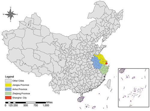
Table 1. Subordination of 41 cities in the Yangtze River Delta.

Name of Province	Name of City^a
Jiangsu	Nanjing	Wuxi	Xuzhou	Huaian	Suzhou (Jiangsu)	Zhenjiang	Lianyungang
	Yancheng	Yanzhou	Nantong	Taizhou (Jiangsu)	Suqian	Changzhou
Zhejiang	Hangzhou	Ningbo	Wenzhou	Jianxing	Huzhou	Shaoxing	Jinhua
	Zhoushan	Taizhou (Zhejiang)	Lishui	Quzhou
Anhui	Hefei	Wuhu	Bengbu	Huainan	Maanshan	Huaibei	Tongling
	Huangshan	Chuzhou	Fuyang	Suzhou (Anhui)	Luan	Bozhou	Chizhou
	Anqing	Xuancheng
Municipalities	Shanghai

^aSince the English names of Taizhou city in Zhejiang province and Taizhou city in Jiangsu province, Suzhou city in Jiangsu province and Suzhou city in Anhui province are the same, so the provinces they belong to are listed behind in this paper to distinguish them.

The spatial distribution characteristics of urban residential land prices in the YRDUA

Figure 3 shows the distribution of residential land prices in cities in the YRDUA.

Figure 3. Spatial heterogeneity diagram of Residential Land Prices in the YRDUA.

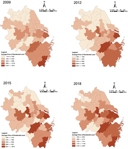
The residential land price in the YRDUA is high in the southeast and low in the northwest. The land price of provincial capital cities and municipalities is the highest, gradually decreasing around central cities. Land prices in Shanghai, Hangzhou, Nanjing, and Suzhou are the highest and have the most apparent radiation effect. Residential land prices across the YRDUA have been increasing over time.

Empirical model specification

Because the core explanatory variable, the average residential land price data under adaptive expectations, which comes from the lagged data of the dependent variable, there is an endogenous problem with the dependent variable. Since there is a lagging one-period term of the dependent variable in the model, it is just in line with the setting of the dynamic panel model. Therefore, the dynamic spatial panel regression model is chosen. Based on the geographical coordinates of 41 cities in the YRDUA, this paper constructs the reciprocal distance spatial contiguity matrix to determine the spatial weight matrix of the model, as shown in formulas (7) and (8); and assumes the spatial weight matrix doesn’t change with time t.

(7) $\begin{array}{c}{\omega }_{ij}=\left\{\begin{array}{c}0\left(i=k\right)\\ \frac{1}{d_{i,j}}\left(i\ne k\right)\end{array}\hspace{0.17em}\right.\end{array}$(7)

(8) $W_{i,j}=\left[\begin{array}{cccc}0& w_{12}& \cdots & w_{1j}\\ w_{21}& 0& \cdots & w_{2j}\\ ⋮& ⋮& \ddots & ⋮\\ w_{i1}& w_{i2}& \cdots & 0\end{array}\right]$(8)

Among them, $i$, $j$ = 1, 2, … , N city; $W_{ij}$ is the spatial weight matrix between city $i$ and city $j$.

Variable selection and data sources

The dependent variable is the average residential land price $AP{R}_{i,t}$, and the core explanatory variables are adaptive expectations ($AP{R}_{i,t-1}$) and land finance($L{F}_{i,t}$), which are the main reasons for the distortion of residential land prices($i$ and $t$ refer to the data of city $i$ in the period of $t$). Since the adaptive expectation is ‘Disaster Myopia’ ^[31], the current period’s price is determined mainly by the price level of the previous period. This paper assumes that the result of the adaptive expectation is always correct. Adaptive expectation measured by the first-order lag term of the average residential land price. Land finance is measured by proportioning land sale revenue in expected fiscal revenue. The increase in the proportion of land sale revenue in expected fiscal revenue means the dependence of local government revenue on land finance has been increasing. The control variables, including the demand and supply of land, economic fundamentals, and government macroeconomic policies, the control variables are:

The demand side includes GDP（$GD{P}_{i,t}$）; per capita disposable income ($PCD{I}_{i,t}$);population density ($P{D}_{i,t}$), measured by the ratio of resident population to total urban area; urbanization level ($U{L}_{i,t}$), measured by the ratio of urban domicile population to total urban population; the RMB loan balance of financial institutions ($L{B}_{i,t}$); industrial structure ($PS{I}_{i,t}$), measured by services output as a proportion of total industry output and traffic level ($H{M}_{i,t}$),measured by expressway mileage.

The supply side includes the urban land area to be developed ($L{D}_{i,t}$), residential construction land supply ($LH{R}_{i,t}$), real estate development intensity coefficient ($ED{I}_{i,t}$) and fiscal decentralization ($F{D}_{i,t}$). The urban developable land area is measured by the urban built-up area minus the urban land area. The residential construction land supply is measured by the ratio of the residential land construction area to the total planned construction land area. The intensity coefficient of real estate development is measured by the proportion of real estate investment in the total fixed assets of the whole society. The intensity coefficient of real estate development is an indicator used by local governments for market monitoring and early warning, which reflects the coordinated development of real estate investment and macro economy; the degree of fiscal decentralization ($F{D}_{i,t}$) reflects the financial pressure of local governments, measured by the proportion of local per capita fiscal expenditure in the central budget per capita. Descriptive statistics of the variables shown in Table 2.

Table 2. Descriptive statistics of the variables.

Variables	Mean	Std.Dev	Min	Max	Nobs	Unit
$AP{R}_{i,t}$,	5027.797	5177.018	418.55	33831.35	410	yuan/m^2
$L{F}_{i,t}$	119.7887	97.44055	5.768767	567.9804	410	10^4 yuan
$L{B}_{i,t}$	3812.142	8360.342	96.7787	67567.94	410	10^4 yuan
$GD{P}_{i,t}$	2215.038	4036.011	112.1841	32679.87	410	10^4 yuan
$PS{I}_{i,t}$	45.4788	8.539878	23.34	69.9	410	%
$PCD{I}_{i,t}$	30226.05	11275.22	11149.34	68034	410	yuan
$P{D}_{i,t}$	697.1587	535.7219	145.29	3826	410	%
$F{D}_{i,t}$	43.93537	35.81817	5.259211	231.0481	410	%
$H{M}_{i,t}$	308.6267	151.7911	32	835.55	410	km
$ED{I}_{i,t}$	18.18319	7.183149	3.375751	48.75709	410	%
$U{L}_{i,t}$	58.7658	12.29332	29.1	89.6	410	%
$LH{R}_{i,t}$	67.80712	143.4676	9.67	1085.53	410	Km^2
$L{D}_{i,t}$	90.55856	6.977971	59.14397	98.84128	410	Km^2

This paper first performs panel data classical linear model regression on variables (see Table 3) to facilitate the setup of the subsequent model, excluding insignificant fiscal decentralization ($F{D}_{i,t}$) and real estate development intensity coefficient ($ED{I}_{i,t}$) and urban land area to be developed ($L{D}_{i,t}$). Therefore, the final indicators determined are: land finance ($L{F}_{i,t}$), the RMB loan balance of financial institutions ($L{B}_{i,t}$), GDP ($GD{P}_{i,t}$), industrial structure ($PS{I}_{i,t}$), per capita disposable income ($PCD{I}_{i,t}$), population density ($P{D}_{i,t}$), traffic level ($H{M}_{i,t}$), urbanization level ($U{L}_{i,t}$), and residential construction land supply ($LH{R}_{i,t}$). The actual data has been supplemented by linear interpolation.

Table 3. Results of classical linear panel data model regression.

Variables	Coefficient	t-stat	p-value
$L{F}_{i,t}$	9.955792***	5.89	0.000
$L{B}_{i,t}$	0.927825***	7.79	0.000
$GD{P}_{i,t}$	−0.87322***	−3.06	0.002
$PS{I}_{i,t}$	133.4985***	5.58	0.000
$PCD{I}_{i,t}$	0.05066**	2.56	0.011
$P{D}_{i,t}$	−2.05079**	−2.55	0.011
$F{D}_{i,t}$	−10.1335	−1.12	0.261
$H{M}_{i,t}$	−3.8253**	−2.06	0.040
$ED{I}_{i,t}$	7.456689	0.33	0.744
$U{L}_{i,t}$	104.5149***	4.53	0.000
$LH{R}_{i,t}$	−6.25112**	−2.18	0.030
$L{D}_{i,t}$	−22.8554	−0.91	0.361
${\mathit{R}}^{\mathbf{2}}$		0.7131
$\mathit{A}d\mathrm{\_}{R}^2$		0.7044

***, **, and * are significance at 1%, 5% and 10% level, and z-value is in brackets.

Data source

GDP ($GD{P}_{i,t}$), per capita disposable income ($PCD{I}_{i,t}$), industrial structure ($PS{I}_{i,t}$) and traffic level ($H{M}_{i,t}$) come from the CEInet Statistics Database; average residential land price ($AP{R}_{i,t}$), residential construction land supply ($LH{R}_{i,t}$), land finance ($L{F}_{i,t}$) come from CRIC Database. The supply of residential construction land ($LH{R}_{i,t}$) is calculated based on the residential construction land area’s ratio to the planned land area. Land finance ($L{F}_{i,t}$) is calculated based on the ratio of land-transferring fees to fiscal revenue; The urban land area to be developed ($L{D}_{i,t}$), population density ($P{D}_{i,t}$), and urbanization level ($U{L}_{i,t}$) come from the Qianzhan database. The actual data has been supplemented by linear interpolation. All the monetary measures involved are deflated by the consumer price index（CPI）To eliminate the impact of inflation.

IV. Results and discussion

Model selection results

In terms of model selection, according to the test procedure provided by,Anselin, Le Gallo, and Jayet (2008) this paper first conducts the Lagrange multiplier statistic test and selects the spatial econometric model according to the test results (see Table 4).

Table 4. Results of Lagrange multiplier statistic test.

Test Statistic	t-Statistic	Probability
LM test no spatial lag	48.4850	0.000
robust LM test no spatial lag	10.4003	0.001
LM test no spatial error	42.5993	0.000
robust LM test no spatial error	4.51460	0.034
R^2		0.8784

According to the test values of Lagrange multiplier statistics in Table 4, it is found that robust LMρ is more significant than robust LMλ (P-SLM = 0.001 < 0.01<P-SEM = 0.034). Therefore, the spatial lag model should be selected and written as:

$AP{R}_{i,t}=\rho \sum _{j=1}^N{W}_{ij}AP{R}_{i,t}+{\theta }_{1}AP{R}_{i,t-1}+{\theta }_2\sum _{j=1}^N{W}_{ij}AP{R}_{i,t-1}+X_{i,t}\beta +u_{i,t}+v_{i,t}$

$X_{i,t}={\alpha }_{1}L{F}_{i,t}+{\alpha }_{2}PGD{P}_{i,t}+{\alpha }_{3}PCD{I}_{i,t}+{\alpha }_{4}U{L}_{i,t}+{\alpha }_{5}PS{I}_{i,t}+{\alpha }_{6}ED{I}_{i,t}+{\alpha }_{7}H{M}_{i,t}+{\alpha }_{8}LH{R}_{i,t}$

(9) $u_{i,t}=c_i+{\phi }_t$(9)

Among them, $i$ = 1,2, … , N cities; $t$ = 1,2, … , T years, $AP{R}_{i,t}$ represents the explained variable of the city $i$ in year$t$, residential land price under adaptive expectations is set as $AP{R}_{i,t-1}$, $X_{i,t}$ represents the explanatory variable of the city $i$ in year $t$, and expressed by formula 2; $u_{i,t}$ represents the individual specific effect of the city $i$ in year $t$; ρ is the regression coefficient of the spatial lag term; $\beta ,{\theta }_1,{\theta }_2,{\alpha }_1,{\alpha }_2,\dots ,{\alpha }_8$ are the parameters to be estimated; $v_{i,t}$ represents the error term of the city $i$ in year $t$, and $v_{i,t}\text{~}\left(0,{\delta }^2\right)$.

The treatment of individual-specific effects  is generally divided into fixed effects and random effects according to the correlation between  and and  represent spatial fixed effects and time fixed effects, respectively. P-value of Hausman test (see Table 5) is less than 0.01, so the fixed effect is selected.  is regarded as a random variable with a mean of 0 and a variance of  to be added into the model.

Table 5. Results of Hausman test of the spatial lag model.

Statistic	Degrees of freedom	Probability
25.8500	10	0.0039

Likelihood Ratio Test shows that both spatial fixed effects and time fixed effects are significant (see Table 6), so the individual double fixed effects should been selected.

Table 6. Results of LR test.

Test Statistic	Statistic	Degrees of freedom	Probability
LR-test joint significance spatial fixed effects	308.8020	41	0.0000
LR-test joint significance time-period fixed effects	55.4701	10	0.0000

Empirical model results

This paper determines the dynamic spatial panel data model of individual double fixed effects and uses MATLAB to perform model regression. The model code adjusted by Yu, de Jong, and Lee (2012) is adopted. The model results shown in Table 7, and the effect decomposition results of the model are shown in Table 8.

Table 7. Results of dynamic spatial panel data model of individual double fixed effects.

Variables	Coefficient	t-stat	p-value
$AP{R}_{t-1}$（${\theta }_1$）	0.267498***	4.865234	0.000001
$L{F}_{i,t}$	0.265580***	9.898656	0.000000
$L{B}_{i,t}$	−0.046416	−0.632307	0.527187
$GD{P}_{i,t}$	0.331754***	3.161609	0.001569
$PS{I}_{i,t}$	0.103432	0.450182	0.652580
$PCD{I}_{i,t}$	0.757024***	2.922129	0.003476
$P{D}_{i,t}$	0.235220	0.972410	0.330847
$H{M}_{i,t}$	−0.093107	−1.314488	0.188682
$U{L}_{i,t}$	−0.415770*	−1.822952	0.068311
$LH{R}_{i,t}$	−0.257278**	−2.508311	0.012131
$\rho$	0.274815**	2.248046	0.024573
${\theta }_2$	0.217028	1.522625	0.127852
$Nobs$		410
$R^2$		0.9019

***, **, and * are significance at 1%, 5% and 10% level.

Table 8. Results of decomposition of dynamic spatial panel data model effects.

Variables	Direct Effects	t-stat	Indirect Effects	t-stat	Total Effects	t-stat
$AP{R}_{t-1}$（${\theta }_1$）	0.1909	4.6971	0.0668	1.7603	0.2577	4.0132
${\theta }_2$	0.2123	1.5237	0.0691	1.1419	0.2814	1.5077
$L{F}_{i,t}$	0.2707	9.5281	0.0957	1.8306	0.3664	5.629
$L{B}_{i,t}$	−0.0475	−0.5601	−0.0168	−0.469	−0.0643	−0.5486
$GD{P}_{i,t}$	0.3611	3.0895	0.1276	1.5444	0.4887	2.809
$PS{I}_{i,t}$	0.0836	0.3695	0.0308	0.3354	0.1144	0.3686
$PCD{I}_{i,t}$	0.8635	2.9068	0.3021	1.5652	1.1656	2.7211
$P{D}_{i,t}$	0.2343	0.9086	0.0819	0.7503	0.3162	0.8977
$H{M}_{i,t}$	−0.1066	−1.3344	−0.0386	−0.9924	−0.1451	−1.2923
$U{L}_{i,t}$	−0.5056	−1.8144	−0.1786	−1.2386	−0.6842	−1.7405
$LH{R}_{i,t}$	−0.283	−2.4915	−0.1002	−1.407	−0.3832	−2.311

It is shown that the elasticity coefficients of residential land price to both adaptive expectation and land finance are positive and significant, indicating the rising residential land price in the YRDUA in the past ten years, due to the increasing adaptive expectations of real estate developers and the increasing dependence of local governments on land finance. Results show that for every 1% increase in land finance, the residential land price will rise by 0.21%. At the same time, due to the continuous increase in the residential land price, leading to the rise of real estate price, the market generally had the consensus that housing price was uncontrollable, and the government would not effectively inhibit the housing price rise for the sake of economic growth. This market consensus caused real estate to become an essential investment method in China since 2008. It might also be one of the reasons for the failure of the PBOC 4 trillion-yuan economic stimulus plan in 2008. In the model, for every 1% increase in the demand side’s adaptive expectation for the residential land price, the residential land price will rise by 0.30%, and this increasing adaptive expectation will lead to the ratchet effect of housing prices, which in turn will drive the rising residential land price.

The model results show that residential land prices receive adaptive expectations and land finance effects from a spatial perspective. In particular, the spatial auto-correlation coefficient $\rho$ is positive and significant, indicating that residential land price has a positive spatial spillover effect. In the YRDUA, the developable land in municipalities, provincial capitals, and sub-provincial cities is reducing year by year, then these small and medium-sized cities around the big cities are favoured by real estate developers; along with the progress of urban agglomeration in the YRDUA, the increase in adaptive expectations ($AP{R}_{t-1}$) makes real estate developers no longer only focus on local cities when purchasing residential land but are equally optimistic about the surrounding areas with development potential. Therefore, real estate developers’ demand for residential land spreads to neighbouring cities with similar economic development and living environment. Although this spread will ease the tension of urban residential land to a certain extent, it will also increase the residential land price in surrounding cities, resulting in high land prices within a specific scope. Small and medium-sized cities around Shanghai, Hangzhou, Nanjing, Suzhou, and Ningbo, among other big cities, have witnessed rising residential land price over the past decade, and they are becoming less distant from big cities. Similarly, land finance also has a positive spillover effect on the surrounding areas.

It is interesting to note that Table 8 also shows that local land finance policies not only promote local residential land prices, but also drive up residential land prices in the surrounding areas. For governments in neighbouring cities, this means that perhaps even though these governments are trying to control residential land prices, residential land prices will still change as a result of the policies of the central city government. This suggests that the actions of local governments influence each other. This phenomenon can be explained in two ways. Firstly, the Chinese central government rewards and punishes local officials according to their economic performance, so the local Chinese officials will Otherwise, other officials will eliminate them and lose their professional promotion qualification. To compete for promotion, a radical stronger land finance policy in the central city will have a ‘demonstration effect’ on the surrounding areas, thus reinforcing this path to higher finance. Secondly, For real estate developers, when the marginal cost is greater than the marginal income, it is impracticable to purchase high-cost residential land so they will turn to the surrounding areas. These new investments in surrounding areas will continue to drive the growth of the residential land price. Adaptive expectations and land finance interact and influence each other, causing the residential land price to rise and spread to the neighbouring city.

Apart from the core explanatory variable, the remaining control variables align with the expected situation. The regression coefficients of gross domestic products (GDP) and per capita disposable income (PCDI) are positive and significant (α = 0.01). Economic development and the increase in PCDI drive residential land prices. Urbanization level ($U{L}_{i,t}$), and residential construction land supply ($LH{R}_{i,t}$) are significant (α = 0.01, 0.05). The increase of $U{L}_{i,t}$ means that more rural land is included in urban land planning; the increase of $LH{R}_{i,t}$ means an increase in the supply of residential land, so both are helpful in alleviating the rise of residential land prices.

Endogenous and robustness test

This paper chooses to replace the robustness test’s geographical weights and instrumental variables method.

The government determines the base price of residential land price, so the government will tend to raise the base price of residential land under the incentive of land finance, indicating that the relationship between land finance and residential land price is endogenous. This paper selects land use tax ($LU{T}_{i,t}$)as an instrumental variable for regression, which is obtained by multiplying the land use area and tax rate, to address the endogeneity issue. Land finance and land use tax are correlated, but the increase in land use tax is only thought to be an increase in land supply and does not reflect the land price change. Land finance and land area use tax are correlated, but the increase in land construction use tax is only thought to be an increase in land supply and does not reflect the land price change, so it is not related to the explanatory variables.

The spatial spillover effect of the land price depends on spatial distance and the close economic ties between different regions. For example, Nanjing and Yangzhou are spatially closer to the Hefei, but affected more from Shanghai. Therefore, this paper uses the economic matrix to replace the original spatial matrix. After returning the spatial matrix, the model changes from a dual-fixed model to an individual fixed-effect model. The rest of the model settings remain unchanged, meaning that the regression results are robust.

The results are shown in Table 9.

Table 9. Results of robustness test.

Method of replace geographical weights		Method of using instrumental variables
Variables	Coefficient	Variables	Coefficient
$AP{R}_{t-1}$（${\theta }_1$）	0.269916*** (4.919095)	$AP{R}_{t-1}$（${\theta }_1$）	0.451764*** (2.947512)
$L{F}_{i,t}$	0.266756*** (9.882509)	$LU{T}_{i,t}$	0.132761* (1.712113)
$L{B}_{i,t}$	−0.051972 (−0.688164)	$L{B}_{i,t}$	0.076346 (0.899416)
$GD{P}_{i,t}$	0.346898*** (3.274491)	$GD{P}_{i,t}$	0.914513*** (5.394756)
$PS{I}_{i,t}$	0.054071 (0.226022)	$PS{I}_{i,t}$	0.479461 (0.814362)
$PCD{I}_{i,t}$	0.814546*** (3.145147)	$PCD{I}_{i,t}$	0.541214** (2.329416)
$P{D}_{i,t}$	0.147327 (0.62257)	$P{D}_{i,t}$	0.912464 (1.715365)
$H{M}_{i,t}$	−0.062528 (−0.931413)	$H{M}_{i,t}$	0.062528* (−0.931413)
$U{L}_{i,t}$	−0.362614 (−1.636406)	$U{L}_{i,t}$	0.432615 (1.448941)
$LH{R}_{i,t}$	−0.264717*** (−2.587936)	$LH{R}_{i,t}$	0.541295*** (3.597815)
$\rho$	0.126331* (1.939971)	$\rho$	0.354121** (1.979987)
${\theta }_2$	0.159745* (1.688078)	${\theta }_2$	0.238715* (1.751213)
$R^2=0.8566$		R^2 = 0.7294

***, **, and * are significance at 1%, 5% and 10% level.

V. Measurement of distortion of residential land price

Distortion correction coefficient model specification

After identifying the distortion influencing factors of the residential land price, the distortion will lead to the deviation of the residential land price from the reasonable value. Therefore, determining the reasonable residential land value is the key to measuring the degree of distortion, and two problems need to be solved. The first is how to separate the distorting factors from the distorted average residential land price, second is how to reflect the heterogeneity of residential land prices over time and region. Land is a highly heterogeneous commodity, and the Hedonic model is usually used to describe the price of land. The hedonic model can realize the separation of commodity price and commodity characteristics, which is conducive to calculating reasonable residential land prices after removing land distortion factors. Considering the apparent spatial heterogeneity of land prices in YRDUA, this paper considered including GTWR to supplement the Hedonic model to calculate the reasonable urban residential land price with GIS 10.4.1.(Huang, Wu, and Barry 2010; Zhang, Huang, and Zhu 2019; Chai et al. 2021) The model is described as follows:

(10) $\begin{array}{c}AP{R}_{i,t}={\sum }_{i,t}{X}_{i,t}{\delta }_{i,t}\left(u_i,v_i\right)+c_{i,t}\left(u_i,v_i\right)+{\epsilon }_{i,t}\end{array}$(10)

Among them, $X_{i,t}$ refers to the characteristics of residential land in city $i$ during period $t$, it incorporates all the influencing factors both supply and demand as presented in this paper. ${\delta }_{i,t}$ is the corresponding Hedonic price, $c_{i,t}$ is the intercept term, and ${\epsilon }_{i,t}$ is a random error term, $\left(u_i,v_i\right)$ is the geographic coordinate corresponding to each city. Correspondingly, after removing the distortion factors, the new residential land characteristic $X_{i,t}^r$ will be obtained, compared to $X_{i,t}$, $X_{i,t}^r$ is the value after removing the two influencing factors of land finance and adaptive expectations. and the reasonable average price of residential land can be denoted as $AP{R}_{i,t}^r$. Then, the ratio of the reasonable average price of residential land to the distorted average price of residential land can be used to describe the correction coefficients of the degree of distortion of residential land price, which can be expressed as:

(11) $\begin{array}{c}Correctio{n}_{i,t}=\frac{AP{R}_{i,t}^r}{AP{R}_{i,t}}\end{array}$(11)

In the formula, $Correctio{n}_{i,t}$ represents the correction coefficient of city $i$ during period $t$. Considering that there are 410 sample points, 410 correction coefficients can be obtained.

The panel spatio-temporal geographic weighted regression model uses a spatial weight matrix with Gaussian kernel function, which is described as:

(12) $W_{ij}=\frac{1}{\sqrt{2}\pi }{e}^{-\frac{1}{2}{\left(\frac{d_{i,j}}{h_i}\right)}^2}$(12)

Among them, $d_{i,j}$ refers to the distance from city $i$to the city $j$, and $h_i$ is the bandwidth. To better balance the standard deviation and the bias, the bandwidth is adaptive and confirmed by AICc. The regression method is WLS. This paper assumes that $W_{ij}$ does not change with time.

Correction coefficient results

According to the global regression results of various influencing factors in Table 1, the distinguishing factors of GTWR are determined, and results are shown in Table 10.

Table 10. Results of GTWR model.

Variables	Average Value	Minimum Value	Lower Quartile	Upper quartile	Maximum value
$AP{R}_{t-1}$	0.117038	−0.524208	0.255834	−0.031114	0.763177
$L{F}_{i,t}$	0.280155	0.012317	0.349743	0.220070	0.568177
$L{B}_{i,t}$	0.333026	−1.338350	0.668745	0.067394	1.563209
$GD{P}_{i,t}$	0.101143	−1.251689	0.324876	−0.234598	2.127016
$PS{I}_{i,t}$	0.590891	−2.363336	1.080714	−0.116585	5.795098
$PCD{I}_{i,t}$	0.158800	−1.670214	0.473560	−0.200453	2.798831
$P{D}_{i,t}$	0.068020	−0.906631	0.194489	−0.154953	2.043258
$H{M}_{i,t}$	−0.120761	−0.641234	−0.000113	−0.291888	0.783607
$U{L}_{i,t}$	0.205078	−2.468351	0.700724	−0.431253	5.267148
$LH{R}_{i,t}$	−0.137607	−3.487084	0.147456	−0.281512	0.935964
Bandwidth: 0.114996		AICc: 286.473		${\mathbf{R}}^2$: 0.955547

To reflect the difference in the regression coefficients at different time points and different regions in the GTWR model, this paper derives the local regression coefficients of $X_{i,t}$ from the formula (11), and the reasonable average residential land price after excluding the distortion factors, denoted as $AP{R}_{i,t}^r$.The correction coefficient of the local residential land price calculated from the formula (12), denoted as $Correctio{n}_{i,t}$. In the GTWR model, the local regression results of the city $i$ in year$t$ have independent significance. Therefore, whether it is to discuss the regression results of all the cities in year $t$, or to discuss the total regression results of the city $i$ during the 10 years, the results may conceal the individual characteristics of each city in time and space. To better reflect the changes in the correction coefficients of individual units, this paper will directly report $Correctio{n}_{i,t}$ in the form of graphs, the results are shown in Figure 4.

Figure 4. Spatio-temporal variation pattern of the correction coefficients of Residential land prices.

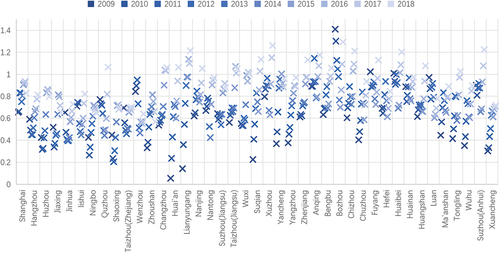
When $Correctio{n}_{i,t}$ = 1, it means that adaptive expectations and land finance do not affect the residential land price in the city i in year t, without distortion; when $Correctio{n}_{i,t}<1$, it means that under the influence of adaptive expectations and land finance, the current residential land price is lower than the reasonable residential land price, and it’s higher when $Correctio{n}_{i,t}>1$. According to Figure 4, the following conclusions can be drawn:

By urban agglomeration, due to adaptive expectations and land finance, the residential land prices in most cities are generally higher than reasonable residential land prices, which means the ‘ratchet effect’ of residential land prices has been formed in these cities. By the year, in 2009, the correction coefficient of residential land cost in each city was generally lower. However, during 2009 –2014, the correction coefficient of each city generally went up and down. It was not until after 2014 that there was a general upward trend, but still below one degree mostly. Analysis of this result in the context of reality, after the 2008 financial crisis, the PBOC issued an investment package worth about 4 trillion yuan to avoid a rapid economic downturn. Although this plan stabilized China’s economy and prevented China economy from collapsing, most of the funds were invested in fixed assets, attracting a swarm of hot money in land and real estate, and speculative demand increased rapidly. This phenomenon directly led to China’s worst ‘money shortage’ of history in June 2013. Therefore, the correction coefficient increased due to adaptive expectations and land finance.

Under the dual pressure of adaptive expectations and land finance, the Chinese central government had to curb the distorted real estate market and issued policy measures such as the ‘Notice of the General Office of the State Council on Continued Regulation of the Real Estate Market’. This policy inhibited the rise of housing prices in various cities, but the lack of incentives for local governments led to a further increase in land prices. After 2014, the Chinese central government proposed removing the GDP assessment system from local officials’ selection. It implemented more stringent real estate control policies and strict ‘destocking’ policies to minimize the impact of various distortions and drove the correction coefficient decline during the period 2014– 2018.

Not all cities’ residential land prices are subject to distortionary factors. By the region, the correction coefficients of cities in Anhui Province are generally higher than in Shanghai, Jiangsu Province and Zhejiang Province, which means that the impact of adaptive expectations and land finance in Anhui Province is slightly. After 2014, the correction coefficient of Jiangsu Province and Anhui Province increased, especially around 2018, the correction coefficient of most cities in Anhui Province, such as Lianyungang, Suqian, Zhenjiang, Anqing, Bozhou, Chizhou, Fuyang, Huaibei, Wuhu, was higher than 1. Local governments took effective policies to curb housing prices, and the central government began to assess local governments with the quality of development around 2015, which has gradually reduced the local government’s financial reliance on land finance. The gradual increase in housing prices also reduced the speculative demand for residential land and lowered the adaptive expectations, residential land more in line with actual supply and demand.

VI. Conclusions

Main conclusions

Theoretical analysis shows a ‘ratchet effect’ on residential land prices in the presence of both adaptive expectations and land finance. When the adaptive expectation and land finance exists, if the residential land market demand is not obvious, the current supply is negatively correlated with the current demand in the current period, and the amount of traded residential land is positively correlated with the residential land price rise. If the residential land market demand is obvious, the current supply is positively correlated with the current demand, and the amount of traded residential land is negatively correlated with the residential land price.

According to the empirical results of the spatial measurement model, this paper finds that the residential land price of the YRDUA has obvious spatial auto-correlation. After regressing the relevant variables, it is found that the spatial spillover effect of adaptive expectation and land finance is significant. Adaptive expectations and land finance have promoted the growth of overall residential land prices in the YRDUA. After further decomposing the results of the model regression, it is found that adaptive expectations and land finance have significantly promoted the growth of local residential land price and peripheral residential land price, which means that the two not only directly promote the growth of local residential land price, but also further promoted the growth of residential land price in neighbouring areas, so it proves that adaptive expectations and land finance are important reasons for the rising residential land price in various cities.

According to the empirical results of the GTWR model, this paper has calculated the correction coefficient of residential land price. This paper believes that adaptive expectations and land finance will lead to abnormal demand and supply, and the residential land price generated under this supply-demand relationship is distorted and frothy. This paper calculates a reasonable residential land price by constructing a GTWR model and derives the residential land price correction coefficient. It is found that in recent years, as the central government tightens the controls and regulations on land policies, the residential land price in the YRDUA gradually becomes more reasonable, reflecting that the policies are effective. In addition, according to the change in the correction coefficient, it is also found that the urban polarization is evident in the YRDUA and that the residential land price of peripheral cities in the YRDUA is slightly lower than reasonable, reflecting that the policies for the integrated construction of the YRDUA must be adapted to local and time conditions.

Future research

The current boundaries of urban agglomeration lack the basis of scientific planning, which are usually focused on GDP or population. In contrast, natural boundaries will cause much differentiated spatial sizes of urban agglomerates; too big or small a scope of urban agglomerates may find it challenging to realize concerted regional development. The correction coefficient may allow the reasonable residential land price to be a zoning reference for urban agglomerates. A reasonable agglomerate may include various land prices in high, medium, and low ends, so how to apply the residential land price correction coefficient to the zoning of urban agglomerates may become the next priority of research.

Acknowledgements

The authors thank the editorial team and anonymous reviewers for their insightful comments on the earlier version of this paper.

Disclosure statement

No potential conflict of interest was reported by the author(s).

Data availability statement

The data and code used in this study are available on request from the first author.

Additional information

Funding

This study was supported by the Central University Basic Research Fund of China (21lzujbkyjh012).

References

- Anselin, L., J. L. Gallo, and H. Jayet 2008. ”Spatial Panel Econometrics.” In The Econometrics of Panel Data. Advanced Studies in Theoretical and Applied Econometrics, edited by L. Mátyás and P. Sevestre. Vol. 46. Berlin, Heidelberg: Springer. doi:10.1007/978-3-540-75892-1_19.
- Bartke, S., and R. Schwarze. 2021. “The Economic Role and Emergence of Professional Valuers in Real Estate Markets.” Land 10 (7): 683. doi:10.3390/land10070683.
- Chai, Z., Y. Yang, Y. Zhao, Y. Fu, and L. Hao. 2021. “Exploring the Effects of Contextual Factors on Residential Land Prices Using an Extended Geographically and Temporally Weighted Regression Model.” Land 10 (11): 1148. doi:10.3390/land10111148.
- Chen, W., Y. Shen, Y. Wang, and Q. Wu. 2018. “How Do Industrial Land Price Variations Affect Industrial Diffusion? Evidence from a Spatial Analysis of China.” Land Use Policy 71: 384–394. doi:10.1016/j.landusepol.2017.12.018.
- Chisholm, M. 1966. “Review of Location and Land Use: Toward a General Theory of Land Rent, by W. Alonso.” Economic Geography 42 (3): 277–279. doi:10.2307/142015.
- Fang, L., C. Tian, X. Yin, and Y. Song. 2018. “Political Cycles and the Mix of Industrial and Residential Land Leasing.” Sustainability 10 (9): 3077. doi:10.3390/su10093077.
- Garang, Z., C. Wu, G. Li, Y. Zhuo, and Z. Xu. 2021. “Spatio-Temporal Non-Stationarity and Its Influencing Factors of Commercial Land Price: A Case Study of Hangzhou, China.” Land 10 (3): 317. doi:10.3390/land10030317.
- Garza, N., and C. Lizieri. 2016. “A Spatial-Temporal Assessment of the Land Value Development Tax.” Land Use Policy 50: 449–460. doi:10.1016/j.landusepol.2015.09.026.
- Higano, Y. 2004. “The Spatial Economy: Cities, Regions, and International Trade.” American Journal of Agricultural Economics 86 (1): 283–285. doi:10.1111/1467-8276.t01-1-00065.
- Hong, Z., Z. Yi, and C. Tiantian. 2016. “Land Remise Income and Remise Price During China’ ‘S Transitional Period from the Perspective of Fiscal Decentralization and Economic Assessment.” Land Use Policy 50: 293–300. doi:10.1016/j.landusepol.2015.10.008.
- Huang, Z., and X. Du. 2021. “How Does High-Speed Rail Affect Land Value? Evidence from China.” Land Use Policy 101: 105068. doi:10.1016/j.landusepol.2020.105068.
- Huang, B., B. Wu, and M. Barry. 2010. “Geographically and Temporally Weighted Regression for Modeling Spatio-Temporal Variation in House Prices.” International Journal of Geographical Information Science 24 (3): 383–401. doi:10.1080/13658810802672469.
- Hunter, W. C., G. G. Kaufman, and M. Pomerleano. 2003. Asset Price Bubbles : The Implications for Monetary, Regulatory, and International Policies. cambridge massachusetts: MIT Press.
- Hu, S., S. Yang, W. Li, C. Zhang, and F. Xu. 2016. “Spatially Non-Stationary Relationships Between Urban Residential Land Price and Impact Factors in Wuhan City, China.” Applied Geography 68: 48–56. doi:10.1016/j.apgeog.2016.01.006.
- Irwin, E. G., and N. E. Bockstael. 2002. “Interacting Agents, Spatial Externalities and the Evolution of Residential Land Use Patterns.” Journal of Economic Geography 2 (1): 31–54. doi:10.1093/jeg/2.1.31.
- Johansen, L. 1967. “The Best Use of Economic Resources.” The Economic Journal 77 (305): 123–124. doi:10.2307/2229360.
- Krause, A. L., and C. Bitter. 2012. “Spatial Econometrics, Land Values and Sustainability: Trends in Real Estate Valuation Research.” Cities 29 (S2): S19–25. doi:10.1016/j.cities.2012.06.006.
- Krugman, P. 1991. “Increasing Returns and Economic Geography.” The Journal of Political Economy 99 (3): 483–499. doi:10.1086/261763.
- Lekachman, R. 1962. “Review of Principles of Economics., by A. Marshall.” Political Science Quarterly 77 (2): 299–300. doi:10.2307/2145893.
- Lerner, A. P. 1936. “A Note on Socialist Economics.” The Review of Economic Studies 4 (1): 72–76. doi:10.2307/2967661.
- Liu, Y., and H. Geng. 2019. “Regional Competition in China Under the Price Distortion of Construction Land: A Study Based on a Two‐regime Spatial Durbin Model.” China & World Economy 27 (4): 104–126. doi:10.1111/cwe.12288.
- Li, Y., and W. Xiong. 2019. “A Spatial Panel Data Analysis of China’s Urban Land Expansion, 2004–2014.” Papers in Regional Science 98 (1): 393–407. doi:10.1111/pirs.12340.
- Ndi, F. A. 2017. “Land Grabbing, Local Contestation, and the Struggle for Economic Gain: Insights from Nguti Village, South West Cameroon.” SAGE Open 7: 215824401668299. doi:10.1177/2158244016682997.
- Wang, R., and J. Hou. 2021. “Land Finance, Land Attracting Investment and Housing Price Fluctuations in China.” International Review of Economics & Finance 72: 690–699. doi:10.1016/j.iref.2020.12.021.
- Wang, J., M. Skidmore, Q. Wu, and S. Wang. 2020. “The Impact of a Tax Cut Reform on Land Finance Revenue: Constrained by the Binding Target of Construction Land.” Journal of Urban Affairs 1–30. doi:10.1080/07352166.2020.1803750.
- Xu, A., C. H. Zhang, and M. Ruther. 2021. “Spatial Dependence and Spatial Heterogeneity in the Effects of Immigration on Home Values and Native Flight in Louisville, Kentucky.” Journal of Urban Affairs 43 (10): 1513–1535. doi:10.1080/07352166.2020.1761257.
- Yang, S., S. Hu, W. Li, C. Zhang, and J. A. Torres. 2017. “Spatiotemporal Effects of Main Impact Factors on Residential Land Price in Major Cities of China.” Sustainability 9 (11): 2050. doi:10.3390/su9112050.
- Yang, S., S. Hu, S. Wang, and L. Zou. 2020. “Effects of Rapid Urban Land Expansion on the Spatial Direction of Residential Land Prices: Evidence from Wuhan, China.” Habitat International 101: 102186. doi:10.1016/j.habitatint.2020.102186.
- Yao, J., X. Zhang, and A. T. Murray. 2018. “Spatial Optimization for Land-Use Allocation: Accounting for Sustainability Concerns.” International Regional Science Review 41 (6): 579–600. doi:10.1177/0160017617728551.
- Ye, F., and W. Wang. 2013. “Determinants of Land Finance in China: A Study Based on Provincial‐level Panel Data.” Australian Journal of Public Administration 72 (3): 293–303. doi:10.1111/1467-8500.12029.
- Yu, J., R. de Jong, and L. F. Lee. 2012. “Estimation for Spatial Dynamic Panel Data with Fixed Effects: The Case of Spatial Cointegration.” Journal of Econometrics 167 (1): 16–37. doi:10.1016/j.jeconom.2011.05.014.
- Zeng, C. 2019. “Spatial Spillover Effect on Land Conveyance Fee—a Multi-Scheme Investigation in Wuhan Agglomeration.” Land Use Policy 89: 104196. doi:10.1016/j.landusepol.2019.104196.
- Zhang, X., B. Huang, and S. Zhu. 2019. “Spatiotemporal Influence of Urban Environment on Taxi Ridership Using Geographically and Temporally Weighted Regression.” ISPRS International Journal of Geo-Information 8 (1): 23. doi:10.3390/ijgi8010023.
- Zhou, J., X. Yu, X. Jin, and N. Mao. 2021. “Government Competition, Land Supply Structure and Semi-Urbanization in China.” Land 10 (12): 1371. doi:10.3390/land10121371.
- Zhou, R., Y. Zhang, and X. Gao. 2021. “The Spatial Interaction Effect of Environmental Regulation on Urban Innovation Capacity: Empirical Evidence from China.” International Journal of Environmental Research and Public Health 18 (9): 4470. doi:10.3390/ijerph18094470.